Modeling Under-Dispersed Count Data by the Generalized Poisson Distribution via Two New MM Algorithms

Abstract

Under-dispersed count data often appear in clinical trials, medical studies, demography, actuarial science, ecology, biology, industry and engineering. Although the generalized Poisson (GP) distribution possesses the twin properties of under- and over-dispersion, in the past 50 years, many authors only treat the GP distribution as an alternative to the negative binomial distribution for modeling over-dispersed count data. To our best knowledge, the issues of calculating maximum likelihood estimates (MLEs) of parameters in GP model without covariates and with covariates for the case of under-dispersion were not solved up to now. In this paper, we first develop a new minimization–maximization (MM) algorithm to calculate the MLEs of parameters in the GP distribution with under-dispersion, and then we develop another new MM algorithm to compute the MLEs of the vector of regression coefficients for the GP mean regression model for the case of under-dispersion. Three hypothesis tests (i.e., the likelihood ratio, Wald and score tests) are provided. Some simulations are conducted. The Bangladesh demographic and health surveys dataset is analyzed to illustrate the proposed methods and comparisons with the existing Conway–Maxwell–Poisson regression model are also presented.

1. Introduction

Under-dispersed count data often appear in clinical trials, medical studies, demography, actuarial science, ecology, biology, industry and engineering. Examples include the number of embryonic deaths in mice in a clinical experiment [1], the number of power outages on each of 648 circuits in a power distribution system in the southeastern United States [2], the number of automotive services purchased on each visit for a customer at a US automotive services firm [3], the species richness that is the simplest measure of species diversity [4], the number of births during a period for women who live in Bangladesh (https://www.dhsprogram.com/data, accessed on 28 January 2022) and so on.

The Poisson distribution is suitable for modeling equally dispersed count data, while the negative binomial distribution is often utilized to model over-dispersed count data. To fit under-dispersed count data, theoretically speaking, researchers should employ the generalized Poisson (GP) distribution because it possesses the twin properties of under- and over-dispersion [5,6,7,8,9,10,11,12,13]. However, in the past 50 years, most authors just treat the GP distribution as an alternative to the negative binomial distribution by eyeing the former’s over-dispersion property, while seeming to ignore its under-dispersion characteristic [6,8,9,10,11,12,13], although Consul & Famoye [6] proved that there exist unique MLEs of parameters for both over- and under-dispersion cases. The main reason for hindering researchers from using the GP distribution with under-dispersion is that calculating the maximum likelihood estimates (MLEs) of parameters in GP models without/with covariates by a stable algorithm is not so easy. To our best knowledge, the issue of calculating MLEs of parameters in the GP model without/with covariates for the case of under-dispersion was not solved up to now; in other words, we may not obtain the correct MLEs of parameters by using the existing algorithms, see Section 5.

A non-negative integer-valued random variable (r.v.) X is said to follow a generalized Poisson (GP) distribution with parameters $\lambda >0$ and $\psi$, denoted by $X\sim \mathrm{G}\mathrm{P}(\lambda ,\psi )$, if its probability mass function (pmf) is given by [5,14]

$$\begin{array}{c}\hfill p\left(x\right|\lambda ,\psi )=\left\{\begin{array}{cc}{\displaystyle \frac{\lambda {(\lambda +\psi x)}^{x-1}{\mathrm{e}}^{-\lambda -\psi x}}{x!},}\hfill & x=0,1,\dots ,\infty ,\hfill \\ 0,\hfill & x>r,\mathrm{when}\psi <0,\hfill \end{array}\right.\end{array}$$

where $max(-1,-\lambda /r)<\psi <1$ and $r(⩾4)$ is the largest positive integer for which $\lambda +\psi r>0$ when $\psi <0$. The expectation and variance of X are given by [14]

$$\begin{array}{c}\hfill E\left(X\right)=\frac{\lambda }{1-\psi }\mathrm{and}\mathrm{Var}\left(X\right)=\frac{\lambda }{{(1-\psi )}^3},\end{array}$$

respectively. The $\mathrm{G}\mathrm{P}(\lambda ,\psi )$ distribution reduces to the $\mathrm{Poisson}\left(\lambda \right)$ when $\psi =0$, and it has the twin properties of over-dispersion when $\psi >0$ and under-dispersion when $\psi <0$.

To formulate the mean regression of the GP distribution, Consul & Famoye [7] introduced a so-called Type I generalized Poisson (${\mathrm{GP}}^{\left(\mathrm{I}\right)}$) distribution, denoted by $Y\sim {\mathrm{GP}}^{\left(\mathrm{I}\right)}(\mu ,\alpha )$, through the following reparameterizations:

$$\begin{array}{c}\hfill \mu =\lambda {(1-\psi )}^{-1}>0\mathrm{and}\alpha ={(1-\psi )}^{-1}.\end{array}$$

(1)

It is easy to show that the pmf of Y is

$$\begin{array}{c}\hfill p\left(y\right|\mu ,\alpha )=\left\{\begin{array}{cc}{\displaystyle \frac{{\displaystyle \mu {[\mu +(\alpha -1)y]}^{y-1}exp\left\{-[\mu +(\alpha -1\left)y\right]/\alpha \right\}}}{{\alpha }^{y}y!},}\hfill & y=0,1,\dots ,\infty ,\hfill \\ 0,\hfill & y>m,\mathrm{when}\alpha <1,\hfill \end{array}\right.\end{array}$$

(2)

where $\mu >0$, $\alpha ⩾max(1/2,1-\mu /m)$ and $m(⩾4)$ is the largest positive integer for which $\mu +(\alpha -1)m>0$ when $\alpha <1$. The mean and variance of Y are given by:

$$E\left(Y\right)=\mu \mathrm{and}\mathrm{Var}\left(Y\right)={\alpha }^2\mu ,$$

respectively, where $\alpha$ denotes the square root of the index of dispersion. The ${\mathrm{GP}}^{\left(\mathrm{I}\right)}(\mu ,\alpha )$ distribution reduces to the $\mathrm{Poisson}\left(\mu \right)$ when $\alpha =1$, and it has the twin properties of over-dispersion when $\alpha >1$ and under-dispersion when $\alpha <1$. Thus, the mean regression model for the ${\mathrm{GP}}^{\left(\mathrm{I}\right)}$ distribution is [7]

$$\begin{array}{c}\hfill {\left\{Y_i\right\}}_{i=1}^n\stackrel{\mathrm{ind}}{\sim }{\mathrm{GP}}^{\left(\mathrm{I}\right)}({\mu }_i,\alpha )\mathrm{and}log\left({\mu }_i\right)={\mathit{w}}_i^{\top }\mathit{\beta },i=1,\dots ,n,\end{array}$$

(3)

where the notation “${\left\{Y_i\right\}}_{i=1}^n\stackrel{\mathrm{ind}}{\sim }{\mathrm{GP}}^{\left(\mathrm{I}\right)}({\mu }_i,\alpha )$” means that $Y_1,\dots ,Y_n$ follow the same ${\mathrm{GP}}^{\left(\mathrm{I}\right)}$ distribution family but with different mean parameters ${\mu }_1,\dots ,{\mu }_n$, and $Y_1,\dots ,Y_n$ are independent; $w_i={(1,w_{i1},\dots ,w_{i,q-1})}^{\top }$ is the covariate vector of subject i and $\mathit{\beta }={({\beta }_0,{\beta }_1,\dots ,{\beta }_{q-1})}^{\top }$ is the vector of regression coefficients.

This paper mainly focuses on developing two new MM algorithms to stably calculate the MLEs of parameters in the ${\mathrm{GP}}^{\left(\mathrm{I}\right)}(\mu ,\alpha )$ distribution with under-dispersion (i.e., $\alpha <1$) and the MLEs of the vector $\mathit{\beta }$ of regression coefficients and the parameter $\alpha$ for the mean regression model in (3). Besides, we want to compare the performance of goodness-of-fit and computational efficiency between the ${\mathrm{GP}}^{\left(\mathrm{I}\right)}$ mean regression model and the Conway–Maxwell–Poisson regression model in simulations and real data analysis.

2. MLEs of Parameters in Generalized Poisson with Under–Dispersion and Its Mean Regression Model

Let ${\left\{Y_i\right\}}_{i=1}^n\stackrel{\mathrm{iid}}{\sim }{\mathrm{GP}}^{\left(\mathrm{I}\right)}(\mu ,\alpha )$ and $Y_{\mathrm{obs}}={\left\{y_i\right\}}_{i=1}^n$ denote the observed counts. Define

$$\begin{array}{ccc}\hfill {\mathbb{I}}_0& \triangleq & \{i:y_i=0,1⩽i⩽n\},\hfill \\ \hfill {\mathbb{I}}_1& \triangleq & \{i:y_i=1,1⩽i⩽n\}\mathrm{and}\hfill \\ \hfill {\mathbb{I}}_2& \triangleq & \{i:y_i⩾2,1⩽i⩽n\}.\hfill \end{array}$$

Let $m_k$ denote the number of elements in ${\mathbb{I}}_k$ for $k=0,1,2$, then we have $m_0+m_1+m_2=n$. Based on (2), the likelihood function of $\{\mu ,\alpha \}$ is

$$\begin{array}{ccc}\hfill L(\mu ,\alpha )& =& \left(\prod _{i\in {\mathbb{I}}_0}{\mathrm{e}}^{-\frac{\mu }{\alpha }}\right)\left(\prod _{i\in {\mathbb{I}}_1}\frac{\mu }{\alpha }{\mathrm{e}}^{-\frac{\mu +\alpha -1}{\alpha }}\right)\hfill \\ & & \times \prod _{i\in {\mathbb{I}}_2}\frac{\mu {[\mu +(\alpha -1)y_i]}^{y_i-1}exp\left\{-[\mu +(\alpha -1)y_i]/\alpha \right\}}{{\alpha }^{y_i}{y}_i!}\hfill \\ & \propto & exp\left(-\frac{m_0\mu }{\alpha }\right)·{\left(\frac{\mu }{\alpha }\right)}^{m_1}exp\left[-\frac{m_1(\mu +\alpha -1)}{\alpha }\right]\hfill \\ & & \times \frac{{\mu }^{m_2}}{{\alpha }^{{\sum }_{i\in {\mathbb{I}}_2}{y}_i}}exp\left\{-\frac{[m_2\mu +(\alpha -1){\sum }_{i\in {\mathbb{I}}_2}{y}_i]}{\alpha }\right\}·\prod _{i\in {\mathbb{I}}_2}{[\mu +(\alpha -1)y_i]}^{y_i-1},\hfill \end{array}$$

where ${\sum }_{i\in {\mathbb{I}}_2}{y}_i=n\overline{y}-m_1$ and $\overline{y}=(1/n){\sum }_{i=1}^n{y}_i$. Then, the log-likelihood function of $\{\mu ,\alpha \}$ is given by

$$\begin{array}{ccc}\hfill \ell (\mu ,\alpha )& =& -\frac{m_0\mu }{\alpha }+m_1[log\left(\mu \right)-log\left(\alpha \right)]-\frac{m_1(\mu +\alpha -1)}{\alpha }+m_{2}log\left(\mu \right)\hfill \\ & & -(n\overline{y}-m_1)log\left(\alpha \right)-\frac{m_2\mu +(\alpha -1)(n\overline{y}-m_1)}{\alpha }\hfill \\ & & +\sum _{i\in {\mathbb{I}}_2}(y_i-1)log\left[y_i(y_i^{-1}\mu +\alpha -1)\right]\hfill \\ & =& (m_1+m_2)log\left(\mu \right)-n\overline{y}log\left(\alpha \right)-\frac{n(\mu -\overline{y})}{\alpha }-n\overline{y}+\sum _{i\in {\mathbb{I}}_2}(y_i-1)log\left(y_i\right)\hfill \\ & & +\sum _{i\in {\mathbb{I}}_2}(y_i-1)log(y_i^{-1}\mu +\alpha -1)\hfill \\ & =& (m_1+m_2)log\left(\mu \right)-n\overline{y}log\left(\alpha \right)-\frac{n(\mu -\overline{y})}{\alpha }\hfill \\ & & +\sum _{i\in {\mathbb{I}}_2}(y_i-1)log(y_i^{-1}\mu +\alpha -1)+c_1,\hfill \end{array}$$

(4)

where $c_1$ is a constant free from $\{\mu ,\alpha \}$.

2.1. MLEs of $\{\mu ,\alpha \}$ via a New MM Algorithm

This subsection aims to find the MLEs of $\{\mu ,\alpha \}$ for the case of $\alpha <1$. Define $y_{max}\triangleq {max}_{i\in {\mathbb{I}}_2}{y}_i$. Because $y_i^{-1}\mu +\alpha -1>0$ for all $i\in {\mathbb{I}}_2$, we have $y_{max}^{-1}\mu +\alpha -1>0$. Thus, we obtain

$$\begin{array}{ccc}\hfill log(y_i^{-1}\mu +\alpha -1)& =& log\left[\left(y_i^{-1}-y_{max}^{-1}\right)\mu +\left(y_{max}^{-1}\mu +\alpha -1\right)\right]\hfill \\ & \stackrel{\left(\mathrm{A}2\right)}{⩾}& v_i^{(t,t)}log\left(\mu \right)+\left(1-v_i^{(t,t)}\right)log[\mu +(\alpha -1)y_{max}]+c_{2i}^{\left(t\right)},\hfill \end{array}$$

(5)

for all $i\in {\mathbb{I}}_2$, where

$$v_i^{(t,t)}\triangleq v_i({\mu }^{\left(t\right)},{\alpha }^{\left(t\right)})and{v}_i(\mu ,\alpha )\triangleq \frac{(y_i^{-1}-y_{max}^{-1})\mu }{y_i^{-1}\mu +\alpha -1},i\in {\mathbb{I}}_2,$$

and $c_{2i}^{\left(t\right)}$ is a constant free from $\{\mu ,\alpha \}$.

By combining (4) and (5), we have

$$\begin{array}{ccc}\hfill \ell (\mu ,\alpha )& ⩾& a_1^{(t,t)}log\left(\mu \right)-n\overline{y}log\left(\alpha \right)-\frac{n(\mu -\overline{y})}{\alpha }+a_2^{(t,t)}log[\mu +(\alpha -1)y_{max}]+c_3^{\left(t\right)}\hfill \\ & \triangleq & Q(\mu ,\alpha |{\mu }^{\left(t\right)},{\alpha }^{\left(t\right)}),\hfill \end{array}$$

which minorizes $\ell (\mu ,\alpha )$ at ${(\mu ,\alpha )}^{\top }={({\mu }^{\left(t\right)},{\alpha }^{\left(t\right)})}^{\top }$, where

$$a_1^{(t,t)}=m_1+m_2+\sum _{i\in {\mathbb{I}}_2}(y_i-1)v_i^{(t,t)},a_2^{(t,t)}=\sum _{i\in {\mathbb{I}}_2}(y_i-1)\left(1-v_i^{(t,t)}\right),$$

and $c_3^{\left(t\right)}$ is a constant free from $\{\mu ,\alpha \}$. Thus, by maximizing $Q(\mu ,\alpha |{\mu }^{\left(t\right)},{\alpha }^{\left(t\right)})$, we have the following MM iterates:

$$\begin{array}{ccc}\hfill {\mu }^{(t+1)}& =& \frac{{\displaystyle a_3\left({\alpha }^{\left(t\right)}\right)+\sqrt{a_3^2\left({\alpha }^{\left(t\right)}\right)+4n(1-1/{\alpha }^{\left(t\right)})y_{max}{a}_1^{(t,t)}}}}{2n}\times {\alpha }^{\left(t\right)}\mathrm{and}\hfill \end{array}$$

(6)

$$\begin{array}{ccc}\hfill {\alpha }^{(t+1)}& =& \frac{a_4\left({\mu }^{(t+1)}\right)+\sqrt{a_4^2\left({\mu }^{(t+1)}\right)+4\left(n\overline{y}-a_2^{(t+1,t)}\right)\times a_5\left({\mu }^{(t+1)}\right)}}{2\left(n\overline{y}-a_2^{(t+1,t)}\right)},\hfill \end{array}$$

(7)

where

$$\begin{array}{ccc}\hfill a_3\left(\alpha \right)& =& -n(1-{\alpha }^{-1})y_{max}+n\overline{y},\hfill \\ \hfill a_4\left(\mu \right)& =& n\mu (1-\overline{y}{y}_{max}^{-1})\mathrm{and}\hfill \\ \hfill a_5\left(\mu \right)& =& n(\mu -\overline{y})(\mu y_{max}^{-1}-1).\hfill \end{array}$$

According to the one-to-one transformation (1), we can obtain the MLEs of $\{\lambda ,\psi \}$ as

$$\widehat{\psi }=1-{\widehat{\alpha }}^{-1}and\widehat{\lambda }={\widehat{\alpha }}^{-1}\widehat{\mu },$$

where $\{\widehat{\mu },\widehat{\alpha }\}$ can be calculated through (6) and (7).

2.2. MLEs of $\{\mathit{\beta },\alpha \}$ in the Mean Regression Model

In this subsection, we consider the mean regression model (3) with $\alpha <1$. Similar to (4), the log-likelihood function of $\{\mathit{\beta },\alpha \}$ is given by

$$\begin{array}{c}\hfill \ell (\mathit{\beta },\alpha )=\sum _{i=1}^n\left\{b_{i1}{\mathit{w}}_i^{\top }\mathit{\beta }-\frac{{\mu }_i-y_i}{\alpha }-y_{i}log\left(\alpha \right)+b_{i2}log(y_i^{-1}{\mu }_i+\alpha -1)\right\}+c_4,\end{array}$$

(8)

where $b_{i1}\triangleq I(y_i⩾1)$, $b_{i2}\triangleq (y_i-1)I(y_i⩾2)$, ${\mu }_i=exp\left({\mathit{w}}_i^{\top }\mathit{\beta }\right)$, and $c_4$ is a constant free from $\{\mathit{\beta },\alpha \}$. The goal is to calculate the MLEs of $\{\mathit{\beta },\alpha \}$.

2.2.1. MLE of $\mathit{\beta }$ Given $\{{\mathit{\beta }}^{\left(t\right)},\alpha \}$

Since $\partial {\mu }_i/\partial \mathit{\beta }={\mu }_i{\mathit{w}}_i$, we have

$$\begin{array}{ccc}\hfill \frac{\partial log(y_i^{-1}{\mu }_i+\alpha -1)}{\partial \mathit{\beta }}& =& \frac{y_i^{-1}{\mu }_i}{y_i^{-1}{\mu }_i+\alpha -1}{\mathit{w}}_i\mathrm{and}\hfill \\ \hfill \frac{{\partial }^{2}log(y_i^{-1}{\mu }_i+\alpha -1)}{\partial \mathit{\beta }\partial {\mathit{\beta }}^{\top }}& =& \frac{(\alpha -1)y_i^{-1}{\mu }_i}{{(y_i^{-1}{\mu }_i+\alpha -1)}^2}{\mathit{w}}_i{\mathit{w}}_i^{\top }.\hfill \end{array}$$

(9)

According to (8), we know that $y_i^{-1}{\mu }_i+\alpha -1>0$, thus $0<1-\alpha <y_i^{-1}{\mu }_i$. Given ${\mathit{\beta }}^{\left(t\right)}$ and $\alpha$, to calculate the $(t+1)$-th approximation of $\widehat{\mathit{\beta }}$, we first restrict $\mathit{\beta }$ in the following convex set

$$\begin{array}{c}\hfill {\mathbb{C}}^{\left(t\right)}=\left\{\mathit{\beta }:y_i^{-1}{\mu }_i⩾T_i^{\left(t\right)}\left(\alpha \right)\triangleq \frac{1}{2}\left[1-\alpha +y_i^{-1}{\mu }_i^{\left(t\right)}\right],\forall i\in {\mathbb{I}}_2\right\},\end{array}$$

(10)

where $T_i^{\left(t\right)}\left(\alpha \right)$ is the midpoint of the two endpoints of the open interval $(1-\alpha ,y_i^{-1}{\mu }_i^{\left(t\right)})$ and ${\mu }_i^{\left(t\right)}\triangleq exp\left({\mathit{w}}_i^{\top }{\mathit{\beta }}^{\left(t\right)}\right)$. Then, for any $i\in {\mathbb{I}}_2$, since $\alpha -1<0$, we have

$$\begin{array}{c}\hfill \frac{(\alpha -1)y_i^{-1}}{{(y_i^{-1}{\mu }_i+\alpha -1)}^2}\stackrel{\left(10\right)}{⩾}\frac{(\alpha -1)y_i^{-1}}{{[T_i^{\left(t\right)}\left(\alpha \right)+\alpha -1]}^2}\triangleq b_{i3}^{\left(t\right)}\left(\alpha \right).\end{array}$$

(11)

On the other hand, we define

$$\begin{array}{c}\hfill h_i^{\left(t\right)}\left(\mathit{\beta }\right|\alpha )=log\left[{\mu }_i+(\alpha -1)y_i\right]-b_{i3}^{\left(t\right)}\left(\alpha \right){\mu }_i,\forall i\in {\mathbb{I}}_2.\end{array}$$

(12)

By combining (9) with (11), we have

$$\frac{{\partial }^2{h}_i^{\left(t\right)}\left(\mathit{\beta }\right|\alpha )}{\partial \mathit{\beta }\partial {\mathit{\beta }}^{\top }}⩾0;$$

i.e., ${\partial }^2{h}_i^{\left(t\right)}\left(\mathit{\beta }\right|\alpha )/\partial \mathit{\beta }\partial {\mathit{\beta }}^{\top }$ is a positive semi-definite matrix. By applying the second-order Taylor expansion of $h_i^{\left(t\right)}\left(\mathit{\beta }\right|\alpha )$ around ${\mathit{\beta }}^{\left(t\right)}$, we have

$$\begin{array}{c}\hfill h_i^{\left(t\right)}\left(\mathit{\beta }\right|\alpha )⩾h_i^{\left(t\right)}\left({\mathit{\beta }}^{\left(t\right)}\right|\alpha )+b_{i4}^{\left(t\right)}\left(\alpha \right)\times {(\mathit{\beta }-{\mathit{\beta }}^{\left(t\right)})}^{\top }{\mathit{w}}_i,\end{array}$$

(13)

where the equality holds iff $\mathit{\beta }={\mathit{\beta }}^{\left(t\right)}$, and $b_{i4}^{\left(t\right)}\left(\alpha \right)\triangleq \{{[{\mu }_i^{\left(t\right)}+(\alpha -1)y_i]}^{-1}-b_{i3}^{\left(t\right)}\left(\alpha \right)\}{\mu }_i^{\left(t\right)}$. Let ${\ell }_1\left(\mathit{\beta }\right|\alpha )$ denote the conditional log-likelihood function of $\mathit{\beta }$ given $\alpha$, we have

$$\begin{array}{ccc}& & {\ell }_1\left(\mathit{\beta }\right|\alpha )\stackrel{\left(8\right)}{=}\ell (\mathit{\beta },\alpha )\hfill \\ & \stackrel{\left(12\right)\&\left(13\right)}{⩾}& \sum _{i=1}^n\left\{\left[b_{i1}+b_{i2}{b}_{i4}^{\left(t\right)}\left(\alpha \right)\right]{\mathit{w}}_i^{\top }\mathit{\beta }-\left[{\alpha }^{-1}-b_{i2}{b}_{i3}^{\left(t\right)}\left(\alpha \right)\right]exp\left({\mathit{w}}_i^{\top }\mathit{\beta }\right)\right\}+c_5^{\left(t\right)}\hfill \\ & \triangleq & Q_1\left(\mathit{\beta }\right|{\mathit{\beta }}^{\left(t\right)},\alpha ),\hfill \end{array}$$

which minorizes ${\ell }_1\left(\mathit{\beta }\right|\alpha )$ at $\mathit{\beta }={\mathit{\beta }}^{\left(t\right)}$, where $c_5^{\left(t\right)}$ is a constant free from $\mathit{\beta }$.

Note that the $Q_1\left(\mathit{\beta }\right|{\mathit{\beta }}^{\left(t\right)},\alpha )$ is a weighted log-likelihood function of $\mathit{\beta }$ for the Poisson regression model with weight vector ${({\alpha }^{-1}-b_{12}{b}_{13}^{\left(t\right)}\left(\alpha \right),\dots ,{\alpha }^{-1}-b_{n2}{b}_{n3}^{\left(t\right)}\left(\alpha \right))}^{\top }$ and observations $Y_{\mathrm{obs}}^{*}={\left\{y_i^{*}\right\}}_{i=1}^n$ with

$$y_i^{*}=\frac{b_{i1}+b_{i2}{b}_{i4}^{\left(t\right)}\left(\alpha \right)}{{\alpha }^{-1}-b_{i2}{b}_{i3}^{\left(t\right)}\left(\alpha \right)},i=1,\dots ,n.$$

We can calculate the MLEs of $\mathit{\beta }$, denoted by ${\mathit{\beta }}_{*}^{(t+1)}$, of the weighted Poisson regression model directly through the built-in ‘glm’ function in the VGAM R package. Since ${\mathit{\beta }}_{*}^{(t+1)}$ is restricted in the convex set ${\mathbb{C}}^{\left(t\right)}$, we project ${\mathit{\beta }}_{*}^{(t+1)}$ on the convex set ${\mathbb{C}}^{\left(t\right)}$, and calculate the $(t+1)$-th approximation of $\widehat{\mathit{\beta }}$ as

$$\begin{array}{ccc}\hfill {\mathit{\beta }}^{(t+1)}& =& {\mathit{\beta }}^{\left(t\right)}+s^{\left(t\right)}({\mathit{\beta }}_{*}^{(t+1)}-{\mathit{\beta }}^{\left(t\right)}),\hfill \end{array}$$

(14)

where

$$\begin{array}{ccc}\hfill s^{\left(t\right)}& \triangleq & min\left(\underset{i\in {\mathbb{I}}_2}{min}{s}_i^{\left(t\right)},1\right)\mathrm{and}\hfill \\ \hfill s_i^{\left(t\right)}& \triangleq & \frac{log\left[T_i^{\left(t\right)}\left(\alpha \right)y_i\right]-{\mathit{w}}_i^{\top }{\mathit{\beta }}^{\left(t\right)}}{{\mathit{w}}_i^{\top }({\mathit{\beta }}_{*}^{(t+1)}-{\mathit{\beta }}^{\left(t\right)})}I({\mathit{w}}_i^{\top }({\mathit{\beta }}_{*}^{(t+1)}-{\mathit{\beta }}^{\left(t\right)})<0)\hfill \\ & & +I({\mathit{w}}_i^{\top }({\mathit{\beta }}_{*}^{(t+1)}-{\mathit{\beta }}^{\left(t\right)})⩾0).\hfill \end{array}$$

2.2.2. MLE of $\alpha$ Given $\{\mathit{\beta },{\alpha }^{\left(t\right)}\}$

Define $T_{min}\left(\mathit{\beta }\right)\triangleq {min}_{i\in {\mathbb{I}}_2}\left(y_i^{-1}{\mu }_i\right)$. Given $\mathit{\beta }$, we have

$$\begin{array}{ccc}\hfill log(y_i^{-1}{\mu }_i+\alpha -1)& =& log\left\{[y_i^{-1}{\mu }_i-T_{min}\left(\mathit{\beta }\right)]+[T_{min}\left(\mathit{\beta }\right)+\alpha -1]\right\}\hfill \\ & \stackrel{\left(\mathrm{A}2\right)}{⩾}& u_i(\mathit{\beta },{\alpha }^{\left(t\right)})log\left[T_{min}\left(\mathit{\beta }\right)+\alpha -1\right]+c_6^{\left(t\right)},\forall i\in {\mathbb{I}}_2,\hfill \end{array}$$

(15)

where $c_6^{\left(t\right)}$ is a constant free from $\alpha$ and

$$u_i(\mathit{\beta },\alpha )\triangleq \frac{T_{min}\left(\mathit{\beta }\right)+\alpha -1}{y_i^{-1}{\mu }_i+\alpha -1}.$$

Let ${\ell }_2\left(\alpha \right|\mathit{\beta })$ denote the conditional log-likelihood function of $\alpha$ given $\mathit{\beta }$, we have

$$\begin{array}{ccc}\hfill & & {\ell }_2\left(\alpha \right|\mathit{\beta })\stackrel{\left(8\right)}{=}\ell (\mathit{\beta },\alpha )\hfill \end{array}$$

$$\begin{array}{ccc}& \stackrel{\left(15\right)}{⩾}& \sum _{i=1}^n\left\{\frac{y_i-{\mu }_i}{\alpha }-y_{i}log\left(\alpha \right)+b_{i2}·u_i(\mathit{\beta },{\alpha }^{\left(t\right)})log\left[T_{min}\left(\mathit{\beta }\right)+\alpha -1\right]\right\}+c_7^{\left(t\right)}\hfill \\ & \triangleq & Q_2\left(\alpha \right|\mathit{\beta },{\alpha }^{\left(t\right)}),\hfill \end{array}$$

which minorizes ${\ell }_2\left(\alpha \right|\mathit{\beta })$ at $\alpha ={\alpha }^{\left(t\right)}$, where $c_7^{\left(t\right)}$ is a constant free from $\alpha$. By setting $\partial Q_2\left(\alpha \right|\mathit{\beta },{\alpha }^{\left(t\right)})/\partial \alpha =0$, we have the following MM iterates:

$$\begin{array}{c}\hfill {\alpha }^{(t+1)}=min({\alpha }_{*}^{(t+1)},1),\end{array}$$

(16)

where

$$\begin{array}{ccc}\hfill {\alpha }_{*}^{(t+1)}& \triangleq & -\frac{d_2(\mathit{\beta },{\alpha }^{\left(t\right)})+\sqrt{b_2^2(\mathit{\beta },{\alpha }^{\left(t\right)})-4d_1(\mathit{\beta },{\alpha }^{\left(t\right)})d_3\left(\mathit{\beta }\right)}}{2d_1(\mathit{\beta },{\alpha }^{\left(t\right)})},\hfill \\ \hfill d_1(\mathit{\beta },\alpha )& \triangleq & \sum _{i=1}^n{b}_{i2}{u}_i(\mathit{\beta },\alpha )-n\overline{y},\hfill \\ \hfill d_2(\mathit{\beta },\alpha )& \triangleq & n[\overline{\mu }-\overline{y}{T}_{min}\left(\mathit{\beta }\right)],\hfill \\ \hfill d_3\left(\mathit{\beta }\right)& \triangleq & n[T_{min}\left(\mathit{\beta }\right)-1](\overline{\mu }-\overline{y}),\hfill \\ \hfill \overline{\mu }& =& \frac{1}{n}\sum _{i=1}^n{\mu }_i.\hfill \end{array}$$

3. Hypothesis Testing

For the ${\mathrm{GP}}^{\left(\mathrm{I}\right)}$ mean regression model (3), suppose that we are interested in testing the following general null hypothesis:

$$H_0:\mathit{C}\mathit{\theta }={\mathit{c}}_r\mathrm{against}{H}_1:\mathit{C}\mathit{\theta }\ne {\mathit{c}}_r,$$

(17)

where $\mathit{C}$ is a known $r\times (q+1)$ matrix with $\mathrm{rank}\left(\mathit{C}\right)=r_0<(q+1)$, $\mathit{\theta }={({\mathit{\beta }}^{\top },\alpha )}^{\top }$ is the vector of parameters and ${\mathit{c}}_r$ is a known $r\times 1$ vector.

3.1. The Likelihood Ratio Test

Let $\ell \left(\mathit{\theta }\right)\triangleq \ell (\mathit{\beta },\alpha )$ be given by (8). The likelihood ratio statistic is given by

$$T_L=2\left[\ell \left(\widehat{\mathit{\theta }}\right)-\ell \left({\widehat{\mathit{\theta }}}_{H_0}\right)\right],$$

(18)

where $\widehat{\mathit{\theta }}$ is the unconstrained MLEs of $\mathit{\theta }$, which can be calculated by the MM algorithm (14) and (16); while ${\widehat{\mathit{\theta }}}_{H_0}$ is the constrained MLEs of $\mathit{\theta }$ under $H_0$. $T_L$ asymptotically follows a chi-squared distribution with $r_0$ degrees of freedom. The corresponding p-value is

$$p_{{}_{\mathrm{L}}}=Pr(T_L>t_L|H_0)=Pr({\chi }^2\left(r_0\right)>t_L),$$

where $t_L$ is the estimated likelihood ratio statistic.

3.2. The Wald Test

The Wald statistic is given by

$$T_W={(\mathit{C}\widehat{\mathit{\theta }}-{\mathit{c}}_r)}^{\top }{\left[\mathit{C}{\mathit{I}}^{-1}\left(\widehat{\mathit{\theta }}\right){\mathit{C}}^{\top }\right]}^{-1}(\mathit{C}\widehat{\mathit{\theta }}-{\mathit{c}}_r),$$

(19)

where $\widehat{\mathit{\theta }}$ denotes the unconstrained MLEs of $\mathit{\theta }$ and $\mathit{I}\left(\widehat{\mathit{\theta }}\right)$ is the Fishier information matrix (see Appendix B) evaluated at $\mathit{\theta }=\widehat{\mathit{\theta }}$. $T_W$ is asymptotically distributed as a chi-squared distribution with $r_0$ degrees of freedom. The corresponding p-value is

$$p_{{}_{\mathrm{W}}}=Pr(T_W>t_W|H_0)=Pr({\chi }^2\left(r_0\right)>t_W),$$

where $t_W$ is the estimated Wald statistic.

3.3. The Score Test

The score statistic is given by

$$T_S={\left[\mathit{s}\left({\widehat{\mathit{\theta }}}_{H_0}\right)\right]}^{\top }{\mathit{I}}^{-1}\left({\widehat{\mathit{\theta }}}_{H_0}\right)\mathit{s}\left({\widehat{\mathit{\theta }}}_{H_0}\right),$$

(20)

where ${\widehat{\mathit{\theta }}}_{H_0}$ denotes the constrained MLEs of $\mathit{\theta }$ under $H_0$, and

$$\mathit{s}\left(\mathit{\theta }\right)\triangleq \frac{\partial \ell \left(\mathit{\theta }\right)}{\partial \mathit{\theta }}={\left(\frac{\partial \ell \left(\mathit{\theta }\right)}{\partial {\beta }_0},\frac{\partial \ell \left(\mathit{\theta }\right)}{\partial {\beta }_1},\dots ,\frac{\partial \ell \left(\mathit{\theta }\right)}{\partial {\beta }_{q-1}},\frac{\partial \ell \left(\mathit{\theta }\right)}{\partial \alpha }\right)}^{\top },$$

with details being presented in Appendix B. $T_S$ is asymptotically distributed as a chi-squared distribution with $r_0$ degrees of freedom. The corresponding p-value is

$$p_{{}_{\mathrm{S}}}=Pr(T_S>t_S|H_0)=Pr({\chi }^2\left(r_0\right)>t_S),$$

where $t_S$ is the estimated score statistic.

4. Simulations

4.1. Accuracy of MLEs of Parameters

To investigate the accuracy of MLEs of parameters, we consider dimensions: $q=2,4$. The sample sizes are set to be $n=100,200,400$; $\alpha =0.6,0.8,0.95$ and other parameters are set as follows:

(A1)

When $q=2$, $\mathit{\beta }={(1,-1)}^{\top }$; ${\mathit{w}}_i={(1,w_{i1})}^{\top }$, ${\left\{w_{i1}\right\}}_{i=1}^n\stackrel{\mathrm{iid}}{\sim }N(0.3,{\sigma }_0^2)$ with ${\sigma }_0^2=0.5$;

(B1)

When $q=4$, $\mathit{\beta }={(1,-1,2,-2)}^{\top }$; ${\mathit{w}}_i={(1,w_{i1},w_{i2},w_{i3})}^{\top }$, ${\left\{w_{i1}\right\}}_{i=1}^n\stackrel{\mathrm{iid}}{\sim }N(0.3,0.5)$, ${\left\{w_{i2}\right\}}_{i=1}^n\stackrel{\mathrm{iid}}{\sim }U(0,1)$, ${\left\{w_{i3}\right\}}_{i=1}^n\stackrel{\mathrm{iid}}{\sim }\mathrm{Bernoulli}\left(0.5\right)$.

For a given $\{q,n,\mathit{\beta },\alpha \}$, we first generate ${\left\{{\mathit{w}}_i\right\}}_{i=1}^n$, and then generate ${\{Y_i=y_i\}}_{i=1}^n\stackrel{\mathrm{iid}}{\sim }{\mathrm{GP}P}^{\left(\mathrm{I}\right)}({\mathit{w}}_i^{\top }\mathit{\beta },\alpha )$ by the inversion method [15] based on the pmf given by (2). Then, we can calculate the MLEs $\{\widehat{\mathit{\beta }},\widehat{\alpha }\}$ via the MM algorithm (14) and (16) with the generated ${\left\{y_i\right\}}_{i=1}^n$ and corresponding covariate vectors ${\left\{{\mathit{w}}_i\right\}}_{i=1}^n$. Finally, we independently repeat this process 10,000 times.

The resultant average bias (denoted by Bias; i.e., average MLE minus the true value of the parameter) and the mean square error (denoted by MSE; i.e., Bias² + (standard deviation)${}^2$, the standard deviation is estimated by the sample standard deviation of 10,000 MLEs) are reported in Table 1 and Table 2.

Table 1. Parameter estimates based on 10,000 replications for Case (A1).

n	Para	$\mathit{\alpha }=0.6$		$\mathit{\alpha }=0.8$		$\mathit{\alpha }=0.95$
		Bias	MSE	Bias	MSE	Bias	MSE
100	${\beta }_0$	−0.0017	0.0371	−0.0034	0.0494	−0.0044	0.0582
	${\beta }_1$	−0.0011	0.0703	−0.0001	0.0966	−0.0003	0.1186
	$\alpha$	−0.0085	0.0394	−0.0100	0.0535	−0.0187	0.0556
200	${\beta }_0$	−0.0007	0.0260	−0.0007	0.0350	−0.0020	0.0415
	${\beta }_1$	0.0003	0.0543	−0.0001	0.0764	−0.0001	0.0916
	$\alpha$	−0.0037	0.0280	−0.0051	0.0373	−0.0084	0.0417
400	${\beta }_0$	−0.0004	0.0183	−0.0003	0.0242	−0.0009	0.0292
	${\beta }_1$	0.0004	0.0357	0.0000	0.0484	−0.0006	0.0589
	$\alpha$	−0.0014	0.0202	−0.0028	0.0267	−0.0042	0.0314

Table 2. Parameter estimates based on 10,000 replications for Case (B1).

n	Para	$\mathit{\alpha }=0.6$		$\mathit{\alpha }=0.8$		$\mathit{\alpha }=0.95$
		Bias	MSE	Bias	MSE	Bias	MSE
100	${\beta }_0$	0.0011	0.0766	−0.0043	0.1050	−0.0075	0.1248
	${\beta }_1$	0.0034	0.0612	0.0001	0.0815	−0.0010	0.0990
	${\beta }_2$	−0.0063	0.1172	0.0026	0.1593	0.0057	0.1917
	${\beta }_3$	0.0016	0.0622	0.0007	0.0848	0.0003	0.1021
	$\alpha$	−0.0122	0.0421	−0.0189	0.0542	−0.0264	0.0580
200	${\beta }_0$	−0.0001	0.0547	−0.0018	0.0743	−0.0018	0.0897
	${\beta }_1$	0.0004	0.0474	0.0002	0.0655	0.0000	0.0781
	${\beta }_2$	−0.0018	0.0767	0.0014	0.1039	0.0001	0.1256
	${\beta }_3$	0.0003	0.0436	−0.0019	0.0606	−0.0005	0.0722
	$\alpha$	−0.0060	0.0291	−0.0100	0.0377	−0.0132	0.0429
400	${\beta }_0$	−0.0001	0.0363	−0.0006	0.0502	−0.0016	0.0610
	${\beta }_1$	0.0015	0.0297	0.0004	0.0410	0.0001	0.0487
	${\beta }_2$	−0.0004	0.0511	0.0000	0.0707	0.0004	0.0861
	${\beta }_3$	0.0002	0.0297	0.0004	0.0417	−0.0001	0.0498
	$\alpha$	−0.0029	0.0208	−0.0048	0.0269	−0.0063	0.0313

Table 1 and Table 2 showed that the absolute values of Bias and MSE tend to zero with the growth of data size for each parameter in Cases (A1) and (B1). For fixing else parameters, the absolute values of Bias and MSE are small for a small $\alpha$.

4.2. Hypothesis Testing

In this subsection, we explore the performances of the likelihood ratio, Wald and score statistics presented in (18)–(20) for the hypothesis testing in (17) with various parameter configurations. The sample sizes are set to be $n=50\left(50\right)400$, where $n_1\left(s\right)n_2$ means from $n_1$ to $n_2$ with step size s, and other parameters are set as follows:

(A2)

When $q=2$, $\mathit{\beta }={({\beta }_0,{\beta }_1)}^{\top }$, $\alpha$ is set to be $0.75,0.85,0.95$, $\mathit{C}=\left(010\right)$, ${\mathit{c}}_r=0$ and $\mathit{\theta }={({\mathit{\beta }}^{\top },\alpha )}^{\top }$, so that (17) becomes $H_0:{\beta }_1=0$. The true value of $\mathit{\beta }$ in $H_0$ is $\mathit{\beta }={(1,0)}^{\top }$, while the value of $\mathit{\beta }$ in $H_1$ is $\mathit{\beta }={(1,0.5)}^{\top }$. We generate ${\left\{w_{i1}\right\}}_{i=1}^n\stackrel{\mathrm{iid}}{\sim }N(0.1,0.2)$ and set ${\mathit{w}}_i={(1,w_{i1})}^{\top }$;

(B2)

When $q=4$, $\mathit{\beta }={({\beta }_0,{\beta }_1,{\beta }_2,{\beta }_3)}^{\top }$, $\alpha$ is set to be $0.75,0.85,0.95$,

$$\mathit{C}=\left(\begin{array}{ccccc}\hfill 0& \hfill 1& \hfill -1& \hfill 0& \hfill 0\\ \hfill 0& \hfill 0& \hfill 1& \hfill -1& \hfill 0\\ \hfill 0& \hfill 0& \hfill 0& \hfill 1& \hfill 0\end{array}\right),{\mathit{c}}_r=\mathbf{0}{\mathbf{0}}_{3}and\mathit{\theta }={({\mathit{\beta }}^{\top },\alpha )}^{\top },$$

so that (17) becomes $H_0:{\beta }_1={\beta }_2={\beta }_3=0$. The true value of $\mathit{\beta }$ in $H_0$ is $\mathit{\beta }={(1,0,0,0)}^{\top }$ and the value of $\mathit{\beta }$ in $H_1$ is $\mathit{\beta }={(1,-1,1,-0.5)}^{\top }$. We generate ${\left\{w_{i1}\right\}}_{i=1}^n\stackrel{\mathrm{iid}}{\sim }N(0.1,0.05)$, ${\left\{w_{i2}\right\}}_{i=1}^n\stackrel{\mathrm{iid}}{\sim }U(0,0.1)$, ${\left\{w_{i3}\right\}}_{i=1}^n\stackrel{\mathrm{iid}}{\sim }0.4\times \mathrm{Bernoulli}\left(0.5\right)$, and set ${\mathit{w}}_i={(1,w_{i1},w_{i2},w_{i3})}^{\top }$;

(A3)

When $q=2$, $\mathit{\beta }={(1,1)}^{\top }$, $\mathit{C}=\left(001\right)$, ${\mathit{c}}_r=1$ and $\mathit{\theta }={({\mathit{\beta }}^{\top },\alpha )}^{\top }$, so that (17) becomes $H_0:\alpha =1$. The alternative values of $\alpha$ in $H_1$ are set as 0.9 and 0.95. We generate ${\left\{w_{i1}\right\}}_{i=1}^n\stackrel{\mathrm{iid}}{\sim }N(1,0.1)$ and set ${\mathit{w}}_i={(1,w_{i1})}^{\top }$;

(B3)

When $q=4$, $\mathit{\beta }={(1,-1,1,-0.5)}^{\top }$, $\mathit{C}=\left(00001\right)$, ${\mathit{c}}_r=1$ and $\mathit{\theta }={({\mathit{\beta }}^{\top },\alpha )}^{\top }$, so that (17) becomes $H_0:\alpha =1$. The alternative values of $\alpha$ in $H_1$ are set as 0.9 and 0.95. We generate ${\left\{w_{i1}\right\}}_{i=1}^n\stackrel{\mathrm{iid}}{\sim }N(0.1,0.05)$, ${\left\{w_{i2}\right\}}_{i=1}^n\stackrel{\mathrm{iid}}{\sim }U(0,0.1)$, ${\left\{w_{i3}\right\}}_{i=1}^n\stackrel{\mathrm{iid}}{\sim }0.4\times \mathrm{Bernoulli}\left(0.5\right)$, and set ${\mathit{w}}_i={(1,w_{i1},w_{i2},w_{i3})}^{\top }$.

All hypothesis testings are conducted at a significant level of 0.05. To calculate the empirical levels of the three tests, we first generate ${\{Y_i=y_i\}}_{i=1}^n\stackrel{\mathrm{ind}}{\sim }{\mathrm{GP}}^{\left(\mathrm{I}\right)}({\mathit{w}}_i^{\top }\mathit{\beta },\alpha )$ under $H_0$. Repeating this process for L (=10,000) times, we obtained $Y_{\mathrm{obs}}^{\left(l\right)}={\{y_1^{\left(l\right)},\dots ,y_n^{\left(l\right)}\}}_{l=1}^L$. Since our MM algorithm (14) & (16) is designed for $\alpha <1$, we apply two-stage method to obtain the MLEs of $\mathit{\theta }$ for the ${\mathrm{GP}}^{\left(\mathrm{I}\right)}$ regression model. In the first stage, we calculate the MLEs $\{\widehat{\mathit{\beta }},\widehat{\alpha }\}$ via the MM algorithm (14) & (16) with the generated ${\left\{y_i\right\}}_{i=1}^n$ and corresponding covariate vectors ${\left\{{\mathit{w}}_i\right\}}_{i=1}^n$. If the estimated $\widehat{\alpha }<1$, implying that the dataset is under-dispersed, we shall keep the estimation result and will not go to the second stage. If the estimated $\widehat{\alpha }=1$, implying that the dataset may be equal- or over-dispersion, we shall go to the next stage; that is recalculating the MLEs $\{\widehat{\mathit{\beta }},\widehat{\alpha }\}$ through the ‘vglm’ function by choosing family as ‘genpoisson1’ in VGAM R package because this function can only calculate the MLEs of the parameter when $\alpha ⩾1$. Let ${\left\{r_j\right\}}_{j=1}^3$ denote the number of rejecting the null hypothesis $H_0$ by the likelihood ratio, Wald and score statistics, respectively. Hence, the actual significance level can be estimated by $r_j/L$ under $H_0$. Similarly, we generate ${\{Y_i=y_i\}}_{i=1}^n\stackrel{\mathrm{ind}}{\sim }{\mathrm{GP}}^{\left(\mathrm{I}\right)}({\mathit{w}}_i^{\top }\mathit{\beta },\alpha )$ under $H_1$. Repeating this process for L (=10,000) times, we obtained $Y_{\mathrm{obs}}^{\left(l\right)}={\{y_1^{\left(l\right)},\dots ,y_n^{\left(l\right)}\}}_{l=1}^L$. The empirical power can be estimated similarly to the empirical level. All results are reported in Table 3, Table 4, Table 5, Table 6, Table 7 and Table 8.

Table 3. The empirical levels of statistics ($T_L$, $T_W$, $T_S$) for Case (A2).

n	$\mathit{\alpha }=0.75$			$\mathit{\alpha }=0.85$			$\mathit{\alpha }=0.95$
	${\mathit{T}}_{\mathit{L}}$	${\mathit{T}}_{\mathit{W}}$	${\mathit{T}}_{\mathit{S}}$	${\mathit{T}}_{\mathit{L}}$	${\mathit{T}}_{\mathit{W}}$	${\mathit{T}}_{\mathit{S}}$	${\mathit{T}}_{\mathit{L}}$	${\mathit{T}}_{\mathit{W}}$	${\mathit{T}}_{\mathit{S}}$
50	0.0530	0.0599	0.0485	0.0521	0.0591	0.0486	0.0530	0.0602	0.0482
100	0.0512	0.0548	0.0487	0.0502	0.0531	0.0485	0.0490	0.0522	0.0468
150	0.0490	0.0508	0.0476	0.0525	0.0538	0.0510	0.0522	0.0544	0.0505
200	0.0514	0.0526	0.0505	0.0545	0.0561	0.0538	0.0515	0.0525	0.0505
250	0.0495	0.0504	0.0488	0.0494	0.0501	0.0481	0.0528	0.0538	0.0517
300	0.0504	0.0515	0.0502	0.0451	0.0468	0.0451	0.0499	0.0509	0.0485
350	0.0545	0.0558	0.0540	0.0510	0.0514	0.0504	0.0503	0.0507	0.0500
400	0.0542	0.0547	0.0532	0.0480	0.0491	0.0477	0.0504	0.0517	0.0498

Table 4. The empirical powers of statistics ($T_L$, $T_W$, $T_S$) for Case (A2).

n	$\mathit{\alpha }=0.75$			$\mathit{\alpha }=0.85$			$\mathit{\alpha }=0.95$
	${\mathit{T}}_{\mathit{L}}$	${\mathit{T}}_{\mathit{W}}$	${\mathit{T}}_{\mathit{S}}$	${\mathit{T}}_{\mathit{L}}$	${\mathit{T}}_{\mathit{W}}$	${\mathit{T}}_{\mathit{S}}$	${\mathit{T}}_{\mathit{L}}$	${\mathit{T}}_{\mathit{W}}$	${\mathit{T}}_{\mathit{S}}$
50	0.2042	0.2252	0.1902	0.1580	0.1768	0.1489	0.1364	0.1505	0.1273
100	0.5457	0.5607	0.5333	0.4236	0.4392	0.4160	0.3387	0.3526	0.3316
150	0.6750	0.6844	0.6669	0.5411	0.5511	0.5340	0.4437	0.4549	0.4368
200	0.7733	0.7805	0.7702	0.6413	0.6519	0.6376	0.5366	0.5438	0.5326
250	0.8995	0.9030	0.8976	0.7986	0.8022	0.7973	0.6789	0.6853	0.6762
300	0.9439	0.9459	0.9420	0.8549	0.8574	0.8523	0.7591	0.7633	0.7564
350	0.9712	0.9719	0.9708	0.9129	0.9147	0.9119	0.8349	0.8371	0.8329
400	0.9903	0.9907	0.9903	0.9557	0.9571	0.9545	0.8975	0.8987	0.8962

Table 5. The empirical levels of statistics ($T_L$, $T_W$, $T_S$) for Case (B2).

n	$\mathit{\alpha }=0.75$			$\mathit{\alpha }=0.85$			$\mathit{\alpha }=0.95$
	${\mathit{T}}_{\mathit{L}}$	${\mathit{T}}_{\mathit{W}}$	${\mathit{T}}_{\mathit{S}}$	${\mathit{T}}_{\mathit{L}}$	${\mathit{T}}_{\mathit{W}}$	${\mathit{T}}_{\mathit{S}}$	${\mathit{T}}_{\mathit{L}}$	${\mathit{T}}_{\mathit{W}}$	${\mathit{T}}_{\mathit{S}}$
50	0.0588	0.0794	0.0439	0.0594	0.0761	0.0449	0.0539	0.0669	0.0405
100	0.0546	0.0648	0.0475	0.0497	0.0568	0.0435	0.0524	0.0579	0.0459
150	0.0523	0.0588	0.0486	0.0505	0.0563	0.0470	0.0492	0.0522	0.0449
200	0.0470	0.0507	0.0421	0.0541	0.0564	0.0506	0.0535	0.0573	0.0501
250	0.0510	0.0545	0.0485	0.0528	0.0547	0.0502	0.0531	0.0556	0.0506
300	0.0525	0.0550	0.0506	0.0501	0.0526	0.0486	0.0498	0.0515	0.0479
350	0.0490	0.0522	0.0476	0.0518	0.0535	0.0502	0.0527	0.0544	0.0510
400	0.0510	0.0527	0.0487	0.0560	0.0571	0.0540	0.0458	0.0474	0.0453

Table 6. The empirical powers of statistics ($T_L$, $T_W$, $T_S$) for Case (B2).

n	$\mathit{\alpha }=0.75$			$\mathit{\alpha }=0.85$			$\mathit{\alpha }=0.95$
	${\mathit{T}}_{\mathit{L}}$	${\mathit{T}}_{\mathit{W}}$	${\mathit{T}}_{\mathit{S}}$	${\mathit{T}}_{\mathit{L}}$	${\mathit{T}}_{\mathit{W}}$	${\mathit{T}}_{\mathit{S}}$	${\mathit{T}}_{\mathit{L}}$	${\mathit{T}}_{\mathit{W}}$	${\mathit{T}}_{\mathit{S}}$
50	0.1629	0.2173	0.1193	0.1310	0.1700	0.0938	0.1124	0.1442	0.0850
100	0.3998	0.4409	0.3523	0.2918	0.3232	0.2576	0.2289	0.2502	0.2027
150	0.5320	0.5598	0.5042	0.3957	0.4186	0.3709	0.3089	0.3280	0.2912
200	0.7670	0.7824	0.7409	0.6148	0.6298	0.5879	0.4893	0.4988	0.4669
250	0.8241	0.8379	0.8096	0.6747	0.6867	0.6605	0.5487	0.5588	0.5337
300	0.8814	0.8887	0.8759	0.7551	0.7654	0.7442	0.6292	0.6381	0.6193
350	0.9657	0.9675	0.9621	0.8895	0.8934	0.8823	0.7897	0.7942	0.7792
400	0.9786	0.9800	0.9775	0.9215	0.9249	0.9199	0.8367	0.8409	0.8310

Table 7. The empirical levels/powers of statistics ($T_L$, $T_W$, $T_S$) for Case (A3).

n	$\mathit{\alpha }=0.9$			$\mathit{\alpha }=0.95$			$\mathit{\alpha }=1$
	${\mathit{T}}_{\mathit{L}}$	${\mathit{T}}_{\mathit{W}}$	${\mathit{T}}_{\mathit{S}}$	${\mathit{T}}_{\mathit{L}}$	${\mathit{T}}_{\mathit{W}}$	${\mathit{T}}_{\mathit{S}}$	${\mathit{T}}_{\mathit{L}}$	${\mathit{T}}_{\mathit{W}}$	${\mathit{T}}_{\mathit{S}}$
50	0.1652	0.2764	0.0737	0.0881	0.1542	0.0445	0.0603	0.0884	0.0494
100	0.2553	0.3641	0.1616	0.0999	0.1548	0.0608	0.0555	0.0672	0.0479
150	0.3562	0.4563	0.2642	0.1203	0.1725	0.0834	0.0525	0.0614	0.0475
200	0.4738	0.5604	0.3814	0.1426	0.1929	0.0993	0.0533	0.0601	0.0498
250	0.5652	0.6446	0.4870	0.1689	0.2152	0.1286	0.0523	0.0587	0.0505
300	0.6560	0.7207	0.5876	0.1901	0.2423	0.1500	0.0516	0.0543	0.0500
350	0.7272	0.7779	0.6710	0.1996	0.2503	0.1623	0.0546	0.0583	0.0520
400	0.7891	0.8332	0.7418	0.2286	0.2765	0.1886	0.0516	0.0573	0.0496

Table 8. The empirical levels/powers of statistics ($T_L$, $T_W$, $T_S$) for Case (B3).

n	$\mathit{\alpha }=0.9$			$\mathit{\alpha }=0.95$			$\mathit{\alpha }=1$
	${\mathit{T}}_{\mathit{L}}$	${\mathit{T}}_{\mathit{W}}$	${\mathit{T}}_{\mathit{S}}$	${\mathit{T}}_{\mathit{L}}$	${\mathit{T}}_{\mathit{W}}$	${\mathit{T}}_{\mathit{S}}$	${\mathit{T}}_{\mathit{L}}$	${\mathit{T}}_{\mathit{W}}$	${\mathit{T}}_{\mathit{S}}$
50	0.2247	0.3832	0.0878	0.1184	0.2194	0.0486	0.0671	0.1288	0.0417
100	0.3124	0.4417	0.1916	0.1238	0.2025	0.0731	0.0581	0.0846	0.0464
150	0.4119	0.5349	0.2957	0.1479	0.2185	0.0968	0.0553	0.0716	0.0487
200	0.5155	0.6211	0.4160	0.1672	0.2349	0.1165	0.0543	0.0679	0.0485
250	0.6117	0.6991	0.5210	0.1857	0.2510	0.1343	0.0541	0.0648	0.0492
300	0.6962	0.7740	0.6167	0.2040	0.2678	0.1595	0.0527	0.0602	0.0488
350	0.7668	0.8228	0.7022	0.2269	0.2918	0.1772	0.0532	0.0602	0.0502
400	0.8152	0.8606	0.7614	0.2558	0.3197	0.2076	0.0464	0.0545	0.0448

Table 3 shows that the significant levels in the three statistics are around 0.05 for different sample sizes. Table 4 shows that the Wald statistic outperforms the likelihood ratio statistic, and the likelihood ratio statistic outperforms the score statistic. At the same time, the differences in the empirical powers among the three tests are very small. So, we can use the likelihood ratio, Wald, and score statistics for the regression hypothesis testing for various values of $\alpha$ when $q=2$. The differences in performance among the three statistics are presented in Figure 1 and Figure 2.

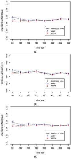
Figure 1. The empirical levels of three test statistics ($T_L$, $T_W$, $T_S$) for testing $H_0:{\beta }_1=0$ in Case (A2) for different $\alpha$. (a) The empirical level with $H_0:\mathit{\beta }={(1,0)}^{\top }$ for $\alpha =0.75$; (b) The empirical level with $H_0:\mathit{\beta }={(1,0)}^{\top }$ for $\alpha =0.85$; (c) The empirical level with $H_0:\mathit{\beta }={(1,0)}^{\top }$ for $\alpha =0.95$.

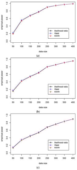
Figure 2. The empirical powers of three test statistics ($T_L$, $T_W$, $T_S$) for testing $H_0:{\beta }_1=0$ in Case (A2) for different $\alpha$’s. (a) The empirical power with $H_1:\mathit{\beta }={(1,0.5)}^{\top }$ for $\alpha =0.75$; (b) The empirical power with $H_1:\mathit{\beta }={(1,0.5)}^{\top }$ for $\alpha =0.85$; (c) The empirical power with $H_1:\mathit{\beta }={(1,0.5)}^{\top }$ for $\alpha =0.95$.

Table 5 shows that the significant level in the likelihood ratio and the score statistics are around 0.05 for different sample sizes, while the significant levels in Wald statistic are around 0.07 for different $\alpha$ when $n=50$ and quickly decrease to 0.05 with the growth of sample size. Table 6 shows that the Wald statistic outperforms the likelihood ratio statistic, and the likelihood ratio statistic outperforms the score statistic. Unlike the differences in the empirical power among the three tests are small in Case (A2), Table 5 shows that the differences are more considerable in Case (B2). So, we can use the likelihood ratio and score statistics for the regression hypothesis testing for various values of $\alpha$ and different samples size when $q=4$. Furthermore, we can use the Wald statistic when the sample size is more than 100. The differences in performance among the three statistics are presented in Figure 3 and Figure 4.

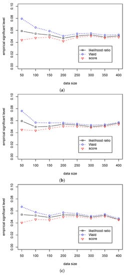
Figure 3. The empirical levels of three test statistics ($T_L$, $T_W$, $T_S$) for testing $H_0:{\beta }_1={\beta }_2={\beta }_3=0$ in Case (B2) for different $\alpha$. (a) The empirical level with $H_1:\mathit{\beta }={(1,0,0,0)}^{\top }$ for $\alpha =0.75$; (b) The empirical level with $H_1:\mathit{\beta }={(1,0,0,0)}^{\top }$ for $\alpha =0.85$; (c) The empirical level with $H_1:\mathit{\beta }={(1,0,0,0)}^{\top }$ for $\alpha =0.95$.

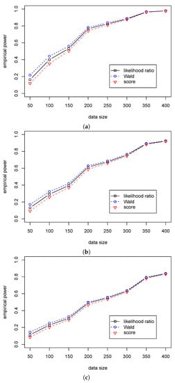
Figure 4. The empirical powers of three test statistics ($T_L$, $T_W$, $T_S$) for testing $H_0:{\beta }_1={\beta }_2={\beta }_3=0$ in Case (B2) for different $\alpha$. (a) The empirical power with $H_1:\mathit{\beta }={(1,-1,1,-0.5)}^{\top }$ for $\alpha =0.75$; (b) The empirical power with $H_1:\mathit{\beta }={(1,-1,1,-0.5)}^{\top }$ for $\alpha =0.85$; (c) The empirical power with $H_1:\mathit{\beta }={(1,-1,1,-0.5)}^{\top }$ for $\alpha =0.95$.

According to Table 7 and Table 8, we can see that the Wald statistic outperforms the other two statistics in Cases (A3)–(B3), and the likelihood ratio statistic outperforms the score statistic. Figure 5 and Figure 6 show a significant difference in empirical power among the three statistics. Furthermore, we can see that the empirical significant levels for the likelihood ratio and score statistics are satisfactorily controlled. In contrast, the significant level for the Wald statistic is over 0.08 when $n=50$ and gradually decreases to 0.05 with the growth of the sample size. So, we suggest using the likelihood ratio statistic for the dispersion hypothesis testing when the sample size is less than 200; and using the Wald statistic when the sample size is more than 200.

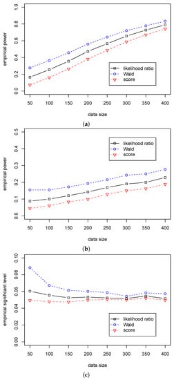
Figure 5. The empirical powers/level of three test statistics ($T_L$, $T_W$, $T_S$) for testing $H_0:{\beta }_1=0$ in Case (A3) for different $\alpha$. (a) The empirical power with $H_1:\mathit{\beta }={(1,1)}^{\top }$ for $\alpha =0.9$; (b) The empirical power with $H_1:\mathit{\beta }={(1,1)}^{\top }$ for $\alpha =0.95$; (c) The empirical significant level with $H_1:\mathit{\beta }={(1,1)}^{\top }$ for $\alpha =1$.

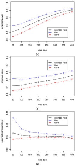
Figure 6. The empirical powers/level of three test statistics ($T_L$, $T_W$, $T_S$) for testing $H_0:{\beta }_1={\beta }_2={\beta }_3=0$ in Case (B3) for different $\alpha$. (a) The empirical power with $H_1:\mathit{\beta }={(1,-1,1,-0.5)}^{\top }$ for $\alpha =0.9$; (b) The empirical power with $H_1:\mathit{\beta }={(1,-1,1,-0.5)}^{\top }$ for $\alpha =0.95$; (c) The empirical significant level with $H_1:\mathit{\beta }={(1,-1,1,-0.5)}^{\top }$ for $\alpha =1$.

4.3. Comparisons of the ${GP}^{\left(I\right)}$ Regression Model with the Conway–Maxwell–Poisson Regression Model

To compare the performance of the goodness-of-fit tests and computational complexity in the ${\mathrm{GP}}^{\left(\mathrm{I}\right)}$ regression model (3) and the Conway–Maxwell–Poisson (CMP) regression model, we consider using both models to fit a dataset, which is generated from one of the two models. A discrete r.v. Y is said to follow the CMP distribution with parameters $\lambda >0$ and $\nu >0$, denoted by $Y\sim \mathrm{CMP}(\lambda ,\nu )$, if its pmf is [16]:

$$\begin{array}{ccc}\hfill Pr(Y=y)& =& \frac{{\lambda }^y}{{(y!)}^{\nu }Z(\lambda ,\nu )},y=0,1,2,\dots ,\infty ,\hfill \end{array}$$

where $Z(\lambda ,\nu )={\sum }_{s=0}^{\infty }{\lambda }^s/{(s!)}^{\nu }$ is a normalizing constant and $\nu$ is the dispersion parameter. The $\mathrm{CMP}(\lambda ,\nu )$ distribution reduces to the $\mathrm{Poisson}\left(\lambda \right)$ when $\nu =1$, and it has the twin properties of over-dispersion when $\nu <1$ and under-dispersion when $\nu >1$. The CMP regression model [3,17] is:

$$\begin{array}{c}\hfill {\left\{Y_i\right\}}_{i=1}^n\stackrel{\mathrm{ind}}{\sim }\mathrm{CMP}({\lambda }_i,\nu )\mathrm{and}log\left({\lambda }_i\right)={\mathit{w}}_i^{\top }\mathit{\beta },i=1,\dots ,n.\end{array}$$

The sample size is set to be $n=1000$, $q=4$, $\mathit{\beta }={(1,-0.5,1,0.5)}^{\top }$, ${\mathit{w}}_i={(1,w_{i1},w_{i2},w_{i3})}^{\top }$, ${\left\{w_{i1}\right\}}_{i=1}^n\stackrel{\mathrm{iid}}{\sim }N(0.1,0.5)$, ${\left\{w_{i2}\right\}}_{i=1}^n\stackrel{\mathrm{iid}}{\sim }U(0,1)$, ${\left\{w_{i3}\right\}}_{i=1}^n\stackrel{\mathrm{iid}}{\sim }\mathrm{Bernoulli}\left(0.5\right)$ and other parameter configurations are set as follows:

(A4)

For a fixed $\mathit{\beta }$, set $\alpha =0.9$ and generate $X_i=x_i\stackrel{\mathrm{ind}}{\sim }{\mathrm{GP}}^{\left(\mathrm{I}\right)}({\mu }_i,\alpha )$ with ${\mu }_i=exp\left({\mathit{w}}_i^{\top }\mathit{\beta }\right)$ for $i=1,\dots ,n$.

(B4)

For a fixed $\mathit{\beta }$, set $\nu =1.2$ and generate $X_i=x_i\stackrel{\mathrm{ind}}{\sim }\mathrm{CMP}({\lambda }_i,\nu )$ with ${\lambda }_i=exp\left({\mathit{w}}_i^{\top }\mathit{\beta }\right)$ for $i=1,\dots ,n$.

To assess the performance of the two models, we use the following three criteria: The average Akaike information criterion (AIC), the average Bayesian information criterion (BIC) and the average Pearson chi-squared statistic ${\chi }_{n-q-1}^2$ [18]:

$${\chi }_{n-q-1}^2=\sum _{i=1}^n\frac{{(x_i-{\widehat{\mu }}_i)}^2}{{\widehat{\sigma }}_i^2},$$

where ${\widehat{\mu }}_i$ and ${\widehat{\sigma }}_i^2$ are the estimated mean and variance of $X_i$ and $(n-q-1)=995$ is the degree of the Pearson chi-squared statistic because we use the MLEs $\{\widehat{\mathit{\beta }},\widehat{\alpha }\}$ or $\{\widehat{\mathit{\beta }},\widehat{\nu }\}$ to calculate ${\{{\widehat{\mu }}_i,{\widehat{\sigma }}_i^2\}}_{i=1}^n$. To show the differences in performance in the two models with the same data set, we first generate a data set from (A4) and estimate parameters with the ${\mathrm{GP}}^{\left(\mathrm{I}\right)}$ and CMP regression models 1000 times. Specifically, we can calculate the MLEs of parameters for the ${\mathrm{GP}}^{\left(\mathrm{I}\right)}$ regression model with the MM Algorithm (14) & (16). The MLEs of parameters of the CMP regression model can be calculated directly through the built-in ‘glm.cmp’ function in the COMPoissonReg R package. Next, we generate another data set from (B4) and estimate these parameters with the two models. By averaging the obtained results, the log-likelihood, AIC, BIC, ${\chi }_{n-p}^2$ and the time cost of the system when the algorithm converged (denoted by Sys. Time) are reported in Table 9.

Table 9. Model comparisons based on 1000 replications for Cases (A4) & (B4).

Case	Model	Log-Likelihood	AIC	BIC	${\mathit{\chi }}_{\mathit{n}-\mathit{p}-1}^2$	Sys. Time
(A4)	${\mathrm{GP}}^{\left(\mathrm{I}\right)}$	−2009.89	4029.77	4054.31	997.07	0.7783 s
	CMP	−2011.14	4032.28	4056.81	999.75	1.2971 s
(B4)	${\mathrm{GP}}^{\left(\mathrm{I}\right)}$	−2157.29	4324.58	4349.12	999.96	1.0038 s
	CMP	−2160.11	4330.21	4354.75	990.26	1.9550 s

Sys. Time represents the averaged time cost of the system when the algorithm converged for each repetition.

According to Table 9, in Case (A4), we can see that the log-likelihood of the ${\mathrm{GP}}^{\left(\mathrm{I}\right)}$ regression model is larger than that of the CMP regression model, and the AIC and BIC of the ${\mathrm{GP}}^{\left(\mathrm{I}\right)}$ regression model are smaller than that of the CMP regression model. However, the values of the log-likelihood, AIC and BIC show an inverse numerical relationship between ${\mathrm{GP}}^{\left(\mathrm{I}\right)}$ and CMP regression models in Case (B4). So, the ${\mathrm{GP}}^{\left(\mathrm{I}\right)}$/CMP regression model performs better log-likelihood, AIC, and BIC when the data is generated from ${\mathrm{GP}}^{\left(\mathrm{I}\right)}$/CMP. For the Pearson chi-squared statistic, the ${\mathrm{GP}}^{\left(\mathrm{I}\right)}$ regression model outperforms the CMP regression model in Case (A4) because the value of ${\mathrm{GP}}^{\left(\mathrm{I}\right)}$ is closer to the degree of the Pearson chi-squared statistic, 995. In Case (B4), the ${\chi }_{n-p-1}^2$ of the ${\mathrm{GP}}^{\left(\mathrm{I}\right)}$ regression model is greater than 995 by around 5, and the ${\chi }_{n-p-1}^2$ of the CMP regression model is less than 995 by around 5, implying they have similar performances. For the cost of time, our proposed ${\mathrm{GP}}^{\left(\mathrm{I}\right)}$ regression model converges faster than the CMP model in simulation, in which the time cost of the ${\mathrm{GP}}^{\left(\mathrm{I}\right)}$ regression model is nearly half of the CMP regression model.

5. Births in Last Five Years for Women in Bangladesh

The dataset is obtained from the Bangladesh demographic and health surveys (DHS) program (https://www.dhsprogram.com/data, accessed on 28 January 2022), recording several variables, e.g., Age, Education (educational level), Religion and Division, from 9067 women who are aged between 30 and 35. Our goal is to understand better the relationship between Births (births in the last five years) and its relevant explanatory variables. In this section, we construct a ${\mathrm{GP}}^{\left(\mathrm{I}\right)}$ regression model to link the mean of Births with the values of Age, Education, Religion and Division and the mean regression model is presented as follows:

$$\begin{array}{ccc}\hfill {\mathsf{Births}}_i& \stackrel{\mathrm{ind}}{\sim }& {\mathrm{GP}}^{\left(\mathrm{I}\right)}({\mu }_i,\alpha ),i=1,\dots ,n,\mathrm{and}\hfill \\ \hfill log\left({\mu }_i\right)& =& {\beta }_0+{\mathsf{Age}}_i\times {\beta }_1+{\mathsf{Primary}}_i\times {\beta }_2+{\mathsf{Secondary}}_i\times {\beta }_3+{\mathsf{Higher}}_i\times {\beta }_4\hfill \\ & & +{\mathsf{Islam}}_i\times {\beta }_5+{\mathsf{Hinduism}}_i\times {\beta }_6+{\mathsf{Chittagong}}_i\times {\beta }_7+{\mathsf{Dhaka}}_i\times {\beta }_8\hfill \\ & & +{\mathsf{Khulna}}_i\times {\beta }_9+{\mathsf{Mymensingh}}_i\times {\beta }_{10}+{\mathsf{Rajshahi}}_i\times {\beta }_{11}\hfill \\ & & ++{\mathsf{Rangpur}}_i\times {\beta }_{12}+{\mathsf{Sylhet}}_i\times {\beta }_{13}.\hfill \end{array}$$

(21)

Meanwhile, for comparisons, we also use the CMP regression model to fit the Bangladesh DHS data

$$\begin{array}{ccc}\hfill {\mathsf{Births}}_i& \stackrel{\mathrm{ind}}{\sim }& CMP({\lambda }_i,\nu ),i=1,\dots ,n,and\hfill \\ \hfill log\left({\lambda }_i\right)& =& {\beta }_0+{\mathrm{Age}}_i\times {\beta }_1+{\mathrm{Primary}}_i\times {\beta }_2+{\mathrm{Secondary}}_i\times {\beta }_3+{\mathrm{Higher}}_i\times {\beta }_4\hfill \\ & & +{\mathrm{Islam}}_i\times {\beta }_5+{\mathrm{Hinduism}}_i\times {\beta }_6+{\mathrm{Chittagong}}_i\times {\beta }_7+{\mathrm{Dhaka}}_i\times {\beta }_8\hfill \\ & & ++{\mathrm{Khulna}}_i\times {\beta }_9+{\mathrm{Mymensingh}}_i\times {\beta }_{10}+{\mathrm{Rajshahi}}_i\times {\beta }_{11}\hfill \\ & & +{\mathrm{Rangpur}}_i\times {\beta }_{12}+{\mathrm{Sylhet}}_i\times {\beta }_{13}.\hfill \end{array}$$

(22)

The MLEs of parameters for the ${\mathrm{GP}}^{\left(\mathrm{I}\right)}$ regression model in (21) can be calculated through the proposed MM algorithm (14) and (16) and the MLEs of parameters for the $\mathrm{CMP}$ regression model in (22) can be calculated through the built-in ‘glm.cmp’ function in the COMPoissonReg R package. For a fixed j ($j=1,\dots ,13$), the Std of ${\widehat{\beta }}_j$ calculated by the Wald statistic for testing $H_0:{\beta }_j=0$ is $\sqrt{{\mathit{e}}_j^{\top }{\mathit{I}}^{-1}\left(\widehat{\mathit{\theta }}\right){\mathit{e}}_j}$, where ${\mathit{e}}_j$ denotes the 15-dimensional vector with 1 for the $(j+1)$-th element and 0’s elsewhere and $\mathit{I}\left(\widehat{\mathit{\theta }}\right)$ is the Fisher information matrix in Appendix B. Thus, the z-values (i.e., MLE/Std) and p-values can be calculated by the MLEs and their Stds and the estimation results of the ${\mathrm{GP}}^{\left(\mathrm{I}\right)}$ and the CMP regression models are presented in Table 10.

Table 10. MLEs and CIs of parameters for the ${\mathrm{GP}}^{\left(\mathrm{I}\right)}$ regression model in (21) and CMP regression model.

	${\mathbf{GP}}^{\left(\mathbf{I}\right)}$				CMP
Parameter	MLE	Std	$\mathit{z}$-Value	$\mathit{p}$-Value	MLE	Std	$\mathit{z}$-Value	$\mathit{p}$-Value
Intercept	4.455	0.3685	12.09	<0.0001	4.843	0.4700	1.31	<0.0001
$\alpha$	0.913	0.0052	−16.71	<0.0001	–	–	–	–
$\nu$	–	–	–	–	1.828	0.0666	27.44	<0.0001
Age	−0.147	0.0097	−15.05	<0.0001	−0.157	0.0121	−12.98	<0.0001
Education
Primary	−0.083	0.0401	−2.06	0.0391	−0.032	0.0508	−0.63	0.5271
Secondary	−0.085	0.0405	−2.10	0.0361	0.002	0.0512	0.04	0.9685
Higher	0.223	0.0534	4.18	<0.0001	0.403	0.0671	6.01	<0.0001
No education	0.000				0.000
Religion
Islam	−0.342	0.1797	−1.90	0.0573	−0.247	0.2387	−1.04	0.3002
Hinduism	−0.638	0.1868	−3.42	0.0006	−0.684	0.2478	−2.76	0.0057
Christianity	0.000				0.000
Division
Chittagong	0.064	0.0551	1.16	0.2461	0.103	0.0685	1.50	0.1331
Dhaka	−0.060	0.0572	−1.05	0.2946	−0.067	0.0711	−0.94	0.3492
Khulna	−0.320	0.0640	−5.00	<0.0001	−0.351	0.0794	−4.42	<0.0001
Mymensingh	0.052	0.0584	0.89	0.3759	0.072	0.0727	0.99	0.3210
Rajshahi	−0.319	0.0630	−5.06	<0.0001	−0.359	0.0781	−4.59	<0.0001
Rangpur	−0.093	0.0597	−1.56	0.1198	−0.116	0.0745	−1.55	0.1208
Sylhet	0.433	0.0540	8.03	<0.0001	0.576	0.0682	8.45	<0.0001
Barisal	0.000				0.000

Table 10 indicates that the Age coefficient is $-0.147$ implying that the Age affects the number of births in the past five years negatively; that is, the willingness to give birth decreases as the growth of ages. The coefficients of Education shows that women with Higher education levels have more births than those with Primary and Secondary education levels. For the religious factor, we realize that there is no significant difference between women, whether Islam, Hinduism, or Christianity. Finally, we can see that the number of births varies widely depending on the Division where they live. More specifically, women who live in Chittagong, Mymensingh and Sylhet are willing to birth more kids, while those who live in Dhaka, Khulna, Rajshahi and Rangpur choose fewer births.

Table 10 shows that there exists minor difference of the coefficients between the ${\mathrm{GP}}^{\left(\mathrm{I}\right)}$ and CMP regression models. The coefficients of Education shows that the Primary and Secondary, respectively, fails to pass the null hypotheses $H_0:{\beta }_2=0$ and $H_0:{\beta }_3=0$ in the CMP regression model under the significant level 5% because their corresponding p-values are both larger than 0.05. However, the two explanatory factors are significant in the ${\mathrm{GP}}^{\left(\mathrm{I}\right)}$ regression model under the above conditions. It deserves to note that the ${\mathrm{GP}}^{\left(\mathrm{I}\right)}$ regression links the mean with the covariate vector directly, so the model is of statistical meaning. However, the CMP regression lacks such statistical meanings because the regression model only constructs a connection between the parameter $\lambda$ with the subject’s personalities.

Furthermore, to have a better understanding of the advantages of the proposed MM algorithm (14) and (16), we apply the existing ‘vglm’ function in VGAM R package to calculate the MLEs $\{\widehat{\mathit{\beta }},\widehat{\alpha }\}$ of the ${\mathrm{GP}}^{\left(\mathrm{I}\right)}$ regression model in (3). Further, we choose two functions ‘genpoisson0’ and ‘genpoisson’ in ‘vglm’ to calculate the MLEs of the parameters, in which the ‘genpoisson0’ function restricts $\alpha ⩾1$ while the ‘genpoisson’ function allows $\alpha >max(1/2,1-\mu /m)$. The criteria for the goodness-of-fit, like AIC, BIC and the Pearson chi-squared statistic, can be calculated by the obtained MLEs, the number of parameters, sample size, and log-likelihoods. The results are presented in Table 11.

Table 11. Comparisons of goodness-of-fit among the ${\mathrm{GP}}^{\left(\mathrm{I}\right)}$ regression model, CMP regression model, log-lambda based GP regression model with constraint $\lambda ⩾0$ and the log-lambda based GP regression model without constraint on $\lambda$.

Model	Log-Likelihood	AIC	BIC	${\mathit{\chi }}_{\mathit{n}-\mathit{p}-1}^2$	Sys. Time
${\mathrm{GP}}^{\left(\mathrm{I}\right)}$	−7624.63	15,279.26	15,385.94	8974.17	11.0384 s
CMP	−7623.66	15,277.32	15,384.01	9017.33	52.4071 s
genpoisson0	−7645.95	15,321.90	15,428.58	7675.93	3.0545 s
genpoisson	−7706.93	15,443.87	15,550.55	7526.34	3.7786 s

genpoisson0 means using the function ‘genpoisson0’ in ‘vglm’; genpoisson means using the function ‘genpoisson’ in ‘vglm’; Sys. Time represents the time cost of the system when the algorithm converged.

Table 11 shows that the ${\mathrm{GP}}^{\left(\mathrm{I}\right)}$ regression model estimated by the proposed MM algorithm and the CMP regression model share similar performance of the goodness-of-fit statistics, like AIC, BIC and Person Chi-square statistic, implying that both models fit the data set well. However, our MM algorithm converges to the $\{\widehat{\mathit{\beta }},\widehat{\alpha }\}$ as nearly five times faster than the ‘glm.cmp’ function for calculating the CMP regression model. We can also see that the log-likelihood, AIC, BIC and ${\chi }_{n-p-1}^2$ obtained through genpoisson0 and genpoisson functions perform much worse than ${\mathrm{GP}}^{\left(\mathrm{I}\right)}$ and CMP regression models, even though they have a relatively less time for computation.

To test the dispersion, we use the likelihood ratio, Wald and score statistics, which have been proved efficiently for large sample sizes in Cases (A3)–(B3) in Section 4.2. The results in Table 12 show that the p-values of the three tests are zeros, implying that the null hypothesis $H_0$: $\alpha =1$ should be rejected.

Table 12. Dispersion test for testing $H_0$: $\alpha =1$.

Tests	Value	p-Value
Likelihood ratio	164.61	<0.0001
Wald	279.27	<0.0001
Score	128.22	<0.0001

6. Discussion

In the present paper, given $\{{\mathit{\beta }}^{\left(t\right)},\alpha \}$, to avoid directly calculating ${\mathit{\beta }}^{(t+1)}$ in the maximization of the original log-likelihood function $\ell (\mathit{\beta },\alpha )$, we successfully constructed a surrogate function $Q_1\left(\mathit{\beta }\right|{\mathit{\beta }}^{\left(t\right)},\alpha )$, which is equivalent to the log-likelihood function in a weighted Poisson regression, so that we can compute ${\mathit{\beta }}_{*}^{(t+1)}$ directly by using the VGAM R package. By projecting ${\mathit{\beta }}_{*}^{(t+1)}$ on the convex set ${\mathbb{C}}^{\left(t\right)}$, we calculated ${\mathit{\beta }}^{(t+1)}$ as shown in (14). Besides, given $\{\mathit{\beta },{\alpha }^{\left(t\right)}\}$, we obtained an explicit expression for ${\alpha }^{(t+1)}$ by maximizing a surrogate function $Q_2\left(\alpha \right|\mathit{\beta },{\alpha }^{\left(t\right)})$. The simulation and real data analysis results showed that the proposed MM algorithms could stably obtain the MLEs of parameters for the ${\mathrm{GP}}^{\left(\mathrm{I}\right)}$ distribution without/with covariates for various parameter configurations, while the built-in ‘genpoisson1’ function in the VGAM R package may converge to a wrong estimate of parameters. Besides, the results of the comparison between the proposed model and the existing CMP regression model reflected that the two models possess similar performance from the aspect of the goodness-of-fit. However, the proposed model outperforms the CMP regression model regarding computational efficiency and statistical meanings.

References

- Saha, K.K. Analysis of one-way layout of count data in the presence of over or under dispersion. J. Stat. Plan. Inference 2008, 138, 2067–2081. [Google Scholar] [CrossRef]
- Guikema, S.D.; Goffelt, J.P. A flexible count data regression model for risk analysis. Risk Anal. Int. J. 2008, 28, 213–223. [Google Scholar] [CrossRef]
- Sellers, K.F.; Borle, S.; Shmueli, G. The COM-Poisson model for count data: A survey of methods and applications. Appl. Stoch. Model. Bus. Ind. 2012, 28, 104–116. [Google Scholar] [CrossRef]
- Lynch, H.J.; Thorson, J.T.; Shelton, A.O. Dealing with under- and over-dispersed count data in life history, spatial, and community ecology. Ecology 2014, 95, 3173–3180. [Google Scholar] [CrossRef]
- Consul, P.C.; Jain, G.C. A generalization of the Poisson distribution. Technometrics 1973, 15, 791–799. [Google Scholar] [CrossRef]
- Consul, P.C.; Famoye, F. The truncated generalized Poisson distribution and its estimation. Commun. Stat.–Theory Methods 1989, 18, 3635–3648. [Google Scholar] [CrossRef]
- Consul, P.C.; Famoye, F. Generalized Poisson regression model. Commun. Stat.-Theory Methods 1992, 21, 89–109. [Google Scholar] [CrossRef]
- Angers, J.F.; Biswas, A. A Bayesian analysis of zero-inflated generalized Poisson model. Comput. Stat. Data Anal. 2003, 42, 37–46. [Google Scholar] [CrossRef]
- Joe, H.; Zhu, R. Generalized Poisson distribution: The property of mixture of Poisson and comparison with negative binomial distribution. Biom. J. 2005, 47, 219–229. [Google Scholar] [CrossRef] [PubMed]
- Yang, Z.; Hardin, J.W.; Addy, C.L.; Vuong, Q.H. Testing approaches for over-dispersion in Poisson regression versus the generalized Poisson model. Biom. J. 2007, 49, 565–584. [Google Scholar] [CrossRef] [PubMed]
- Yang, Z.; Hardin, J.W.; Addy, C.L. A score test for over-dispersion in Poisson regression based on the generalized Poisson-2 model. J. Stat. Plan. Inference 2009, 139, 1514–1521. [Google Scholar] [CrossRef]
- Sellers, K.F.; Morris, D.S. Underdispersion models: Models that are “under the radar”. Commun. Stat.–Theory Methods 2017, 46, 12075–12086. [Google Scholar] [CrossRef]
- Toledo, D.; Umetsu, C.A.; Camargo, A.F.M.; de Lara, I.A.R. Flexible models for non-equidispersed count data: Comparative performance of parametric models to deal with under-dispersion. AStA Adv. Stat. Anal. 2022, 106, 473–497. [Google Scholar] [CrossRef]
- Consul, P.C.; Shoukri, M.M. The generalized Poisson distribution when the sample mean is larger than the sample variance. Commun. Stat.–Theory Methods 1985, 14, 667–681. [Google Scholar] [CrossRef]
- Seber, G.A.F.; Salehi, M.M. Adaptive Sampling Designs: Inference for Sparse and Clustered Populations, Chapter 5: Inverse sampling methods; Springer: New York, NY, USA, 2012. [Google Scholar]
- Shmueli, G.; Minka, T.P.; Kadane, J.B.; Borle, S.; Boatwright, P. A useful distribution for fitting discrete data: Revival of the Conway–Maxwell–Poisson distribution. J. R. Stat. Soc. Ser. C (Appl. Stat.) 2005, 54, 127–142. [Google Scholar] [CrossRef]
- Sellers, K.F.; Shmueli, G. A flexible regression model for count data. Ann. Appl. Stat. 2010, 4, 943–961. [Google Scholar] [CrossRef]
- Cameron, A.C.; Trivedi, P.K. Regression Analysis of Count Data, 2nd ed.; Cambridge University Press: Cambridge, UK, 2013. [Google Scholar]
Disclaimer/Publisher’s Note: The statements, opinions and data contained in all publications are solely those of the individual author(s) and contributor(s) and not of MDPI and/or the editor(s). MDPI and/or the editor(s) disclaim responsibility for any injury to people or property resulting from any ideas, methods, instructions or products referred to in the content. |
© 2023 by the authors. Licensee MDPI, Basel, Switzerland. This article is an open access article distributed under the terms and conditions of the Creative Commons Attribution (CC BY) license (https://creativecommons.org/licenses/by/4.0/).