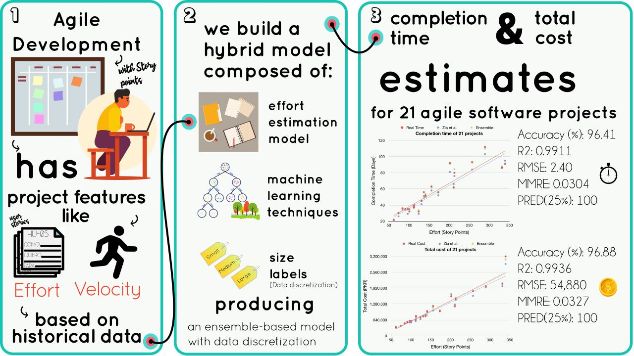
Effort and Cost Estimation Using Decision Tree Techniques and Story Points in Agile Software Development

Abstract

Early effort estimation is important for efficiently planning the use of resources in an Information Technology (IT) project. However, limited research has been conducted on the topic of effort estimation in agile software development using artificial intelligence. This research project contributes to strengthening the use of hybrid models composed of algorithmic models and learning oriented techniques as a project-level effort estimation method in agile frameworks. Effort estimation in agile methods such as Scrum uses a story point approach that measures, using an arithmetic scale, the effort required to complete a release of the system. This project relied on labeled historical data to estimate the completion time measured in days and the total cost of a project set in Pakistani rupees (PKR). using a decision tree, random forest and AdaBoost to improve the accuracy of predictions. Models were trained using 10-fold cross-validation and the relative error was used as a comparison with literature results. The bootstrap aggregation (bagging) ensemble made of the three techniques provides the highest accuracy, and project classification also improves the estimates.

1. Introduction

Software engineering is an important field that focuses on the development of software systems by establishing processes and practices that seek to ensure that projects are developed within scope, cost, time and quality constraints. During a long period of time, the dominant approach for developing projects was the waterfall model, which is a linear, sequential model that begins with analysis and is followed by design, implementation, testing and deployment [1]. Development following a sequential lifecycle is not ideal, as it requires all requirements to be defined upfront, customers do not see working software quickly and it does not adjust to changes in the requirements easily. In the year 2001, a group of software experts proposed a new way of developing software based on a set of principles expressed in an Agile Manifesto that hey created [2]. Agile development gave birth to different methods, one of them being Scrum [3]. Scrum is an iterative project management approach focused on the rapid and early delivery of working software and on adapting to changes in the requirements that occur as the system is being developed.

In Scrum, the project requirements are expressed as a set of user stories that are grouped in a product backlog. At any given moment, the backlog contains all of the unimplemented user stories and, thus, the work that remains to be completed. A user story describes a feature or requirement from the perspective of an end-user or customer. It is a simple, brief and non-technical description that captures the essence of what the user wants to achieve. User stories are described in a short format with the following structure: “As a [user type], I want [goal] so that [reason or benefit]”. This sentence summarizes the user story and is typically accompanied by additional details and acceptance criteria.

Although Scrum considers that the product backlog can be changed at any time, many projects follow a more planned approach, where a number of user stories are considered for a release of the system. These user stories are implemented across a number of iterations called sprints. The release in this case is analogous to a more traditional project, where requirements are relatively stable.

In such a context, it is desirable to be able to produce an accurate early estimate of the effort and cost associated with a product backlog associated with the release project. Early effort estimation allows the project manager to model different scenarios to analyze whether the available resources are sufficient for completing the release project within cost and time constraints. By using proven effort estimation techniques, the team can make decisions based on solid foundations, which directly impact the business. However, when neither an estimation model nor suitable projections are used, this can result in wrong deadlines, as well as a poor quality of the product.

Story points are a size metric used to estimate the effort required to complete user stories. Effort estimation usually takes place at user story level, where the team sets the story points needed to accomplish each user story. The sum of story points for a product backlog allows the project release date and costs to be estimated. In addition, the sum of story points for user stories assigned to particular sprints allows us to calculate the velocity of the team; that is, the average number of story points that a team can typically complete in a given sprint. There are various techniques used in software engineering for estimating. These techniques can be grouped into expert judgment, analogy methods, algorithmic models and machine learning models [4]. Scrum typically promotes an estimation approach called planning poker, where a team uses expert judgement to estimate each user story [5]. If the estimates of the members of the team do not converge for a particular user story, additional estimation rounds are performed until convergence is achieved. While planning poker is a popular technique, it is prone to problems due to biases and team dynamics, and it is also time-consuming. It is thus desirable to perform estimation using alternative approaches that do not suffer from the limitations of planning poker.

In this work, we explored an approach that combines a linear regression model that sets the base for the user stories and the product backlog, generating the dataset that contains all of the projects built with this model. We also applied a discretization of continuous features to label each entry according to their size of effort, time and cost, and supervised machine learning algorithms that take advantage of the data to make estimates of the completion time and total cost. The main idea behind the proposal is the discretization of data and a mix of different decision tree techniques to create an ensemble made of multiple trained models that give an estimate and allow the ensemble to reduce the overall error of averaged estimates. The approach’s limitations are that we have limited data and we depend on the availability of quality data. Historical data might not be useful if there is a changing environment, and they also do not provide any information about the team expertise and experience.

The current work contributes to stressing the importance of data discretization and robust machine learning models in making accurate estimates and reducing the deviation in predictions so that the model sets small intervals, where the team can obtain a better idea of where the real values should be.

This paper is structured as follows. Section 1.1 presents related work that covers some of the research papers that are relevant, including traditional effort estimation and machine learning applied to agile development. Section 1.2 covers the background, including the main concepts of the algorithms applied. Section 2 describes the work proposal for this paper, presenting the procedure for the experiments and the configuration of the machine learning models. Section 3 presents the results of the experiments, comparing the models when data are not labeled and when labels are added. Predictions of the time and cost for all algorithms are plotted to compare their regression line and how far the estimations are from the real values. Finally, the conclusions of the experiments and future work are discussed.

1.1. Related Work

Traditional effort estimation was dominated by expert estimation techniques such as Delphi’s method, the wideband Delphi technique, Work Breakdown Structure (WBS), rule-based systems and the top-down and bottom-up approach [6]. Proposals began in 1950 [7] with regression models. Some of the most common methods used in industry are Software Lifecycle Management (SLIM), the Constructive Cost Model (COCOMO), the Use Case Point (UCP) method and Function Point Analysis (FPA), all of them being introduced in the 1970s and 1980s [8]. Over the years, these models have provided researchers with valuable datasets for building different approaches based on machine learning techniques to provide better estimations. The algorithmic techniques follow mathematical equations, and analogy-based or machine learning techniques are based on a reliable database and can easily be used in the early phase of the project [7,9].

Function-related classifications of Artificial Intelligence (AI) in software engineering are empirically founded and refer to the technologies of AI applied in the software engineering process [10], such as language processing, knowledge management, machine learning and machine vision. In 2012, Wen J. and other researchers suggested machine learning as another category for effort estimation techniques [4].

This category has been growing and several papers propose machine learning models as an alternative to traditional models [11,12,13,14,15,16,17], taking advantage of public datasets such as linear regression trees, random forest, bagging regressor, Adaboost regressor, gradient boosting regressor, k-nearest neighbors, Support Vector Machines (SVMs), intelligent expert systems, fuzzy logic, genetic programming, artificial neural networks and soft computing.

Decision tree analysis dates back to 1931 with Frank P. Ramsey, and, over the past 50 years, much work has been carried out by mathematicians [18]. Its applications cover a great variety of domains, and software engineering is no exception. The interpretability of a Decision Tree (DT) is one of the main reasons for their popularity [19].

A tree model fits a linear regression to the observations, regardless of whether Albrecht, China, Desharnais, Kemerer, Kitchenham, Maxwell or COCOMO datasets are used [20]. In most cases, DT techniques outperform other algorithms such as support vector machines, ridge regression or LASSO regression. In addition, different types of trees can produce low error values and higher prediction values, performing well in some cases in terms of $R^2$ and the Mean Relative Error (MRE) [21,22]. Several studies use a combination of DT with other techniques, and researchers are encouraged to analyze the influence of this combination with the purpose of improving the accuracy of the estimates [23].

The rise of agile methods led to new techniques and metrics, such as planning poker, proposed by Grenning in 2002, and story points, which became widely accepted as a metric used to estimate the size of the work to carry out [24]. Fernandez-Diego et al. [25] presented a systematic literature review on agile software development, pointing out that planning poker, as an expert-based estimation, plays an important role with story points when specifying the requirements of a project. In addition, the study shows that the most frequently used data-based methods are random forests, decision trees, SVM, nearest neighbors, stochastic gradient boosting, naive Bayes and neural networks.

One of the reasons for why AI has not been used widely in agile development is because of a lack of data: in some cases, agile project datasets are private and just a few can be found in various online repositories [26]. Existing effort estimation methods can be classified into expert judgment, algorithmic, machine learning and statistic [27], and, as is known, expert judgment has been widely used since the 1980s. In addition, other metrics have been used within estimation, such as function points and use case points, and studies on machine learning focus on non-agile models [6,16,28,29]. In addition, one of the reasons for the existence of a gap in the ML community and SE community is that each one focuses on their area: a group focuses on algorithms and their performance, whereas the other focuses on software systems [30].

Within the agile effort estimation models with open datasets, we can find the work proposed by Zia et al. [31], whose model was used in this research. The paper intends to calculate the completion time and total cost for the agile software project using a linear-based effort estimation model with a story points approach. A second model that calculates the cost, effort and time needed for a small and medium-sized project using story points was proposed by R. Popli and N. Chauhan [32] in 2014. Another effort to improve estimation accuracy by applying fuzzy logic and a story points estimation model was introduced in 2015 by A.T. Raslan et al. [33].

More models emerged, such as a model for calculating the volume of maintenance in the project, designed to estimate software maintenance effort in terms of the adjusted story point, size, cost and duration [34], or a predictive model that uses developers’ features and SVM to assign story points to issue reports [35]. Other examples proposed by O. Malgonde and K. Chari [36] developed a predictive model for story effort, an ensemble-based approach and an optimization model to optimize available effort using data from the Information Technology (IT) department of a large university, demonstrating the utility of the approach to optimize sprint planning.

Other techniques, such as Principal Component Analysis (PCA) with constraint programming, have measured lower relative error values compared to the planning poker technique applied to data collected from software development firms in various countries [37]. With Bayesian networks, M. Durán et al. [38] represented important factors for a complexity estimation and their relations, with the purpose of helping teams without experience or without historical data, which was a method used to estimate the complexity of user stories. M. Gultekin and O. Kalipsiz [39] used different machine learning algorithms to estimate effort and showed that, when using arithmetic and Fibonacci series as a scoring system, the Fibonacci series gave a better accuracy on estimates combined with the gradient boosting algorithm, outperforming support vector regression, random forest regression and multilayer perceptron.

An ontology model in a multiagent estimation system produces more accurate estimates than methods such as Delphi and planning poker. The system has five agents and is capable of giving information about the sprints required for the project, the average team size, the length of each Scrum phase and the number of features to implement in each sprint, among other information related to the project [40].

A review on Deep Learning (DL) for effort estimation [41] revealed 13 papers from 2017 to 2022, and the findings show that DL techniques are most suitable for effort estimation based on user story textual requirements. Some of the techniques identified are Recurrent Neural Networks (RNNs), Long Short-Term Memory (LSTM), Bi-directional LSTM, Gated Recurrent Units (GRUs), Recurrent Highway Networks (RHNs), Convolutional Neural Networks (CNNs), autoencoders, a deep learning model called BERT grounded on the Transformer language representation model, Text Graph Neural Networks (Text GNNs) and Heterogeneous Graph Neural Networks (HGNNs). All of these approaches are more effective in learning and capturing the semantic and syntactic features from textual data.

An example of a DL approach is given by Morakot Choetkiertikul et al. [42], who proposed a prediction model called a Deep learning model for Story point Estimation (Deep-SE) for estimating story points based on an LSTM network and an RHN. The LSTM extracts features from user stories and a feed forward neural network with a linear activation function performs the final regression to produce a story point estimate.

Finally, we focus on a set of works that have the dataset [31] used to train the machine learning algorithms and produce estimates in common. All of these proposals compete with our approach to determine which technique gives the best results. We list 11 papers in

Table 1. Extending Table 1 from [54], we summarize the studies that train the algorithms using Zia et al. [31] dataset.

No	Title	Input	Output	Technique	Pred(%)	Evaluation Criteria	MSE/RMSE	${\mathit{R}}^2$	MMRE/MMER
1	An Effort Estimation Model for Agile Software Development [31]	No of User Stories, Team Velocity, Sprint Size, No of Working days per Month, Team Salary, Confidence Level in Estimation	Effort, Init Velocity, Friction Factors, Dynamic Forces, Deceleration, Velocity, Time and Cost	Linear-based regression model	Time: 57.14	Mean Magnitude of Relative Error (MMRE), PRED(7.19)	NA	NA	7.19
					Cost: 61.90	MMRE PRED(5.76)	NA	NA	5.76
2	Empirical Validation of Neural Network Models for Agile Software Effort Estimation based on Story Points [43]	Effort, Velocity	Completion Time	General Regression Neural Network (GRNN)	85.9182	Mean Square Error (MSE), Squared correlation coefficient $\left(R^2\right)$, MMRE, Prediction Accuracy (PRED)	0.0244	0.7125	0.3581
				Probabilistic Neural Network (PNN)	87.6561		0.0276	0.6614	1.5776
				Group Method of Data Handling Polynomial Neural Network (GMDH-PNN)	89.6689		0.0317	0.6259	0.1563
				Cascade-Correlation Neural Network (CCNN)	94.7649		0.0059	0.9303	0.1486
3	An Agile Effort Estimation Based on Story Points Using Machine Learning Techniques [45]	Effort, Velocity	Completion Time, Total Cost	Adaptive Neuro-Fuzzy Interface System (ANFIS)	Time: 76.19 Cost: 57.14	MMRE, Mean of Magnitude of Error Relative (MMER), PRED(x)	NA	NA	Time: 8.4277 Cost: 3.9079
				Generalized Regression Neural Networks (newGRNN)	76.1905		NA	NA	Time: 2.7864 Cost: 4.8335
				Radial Basis Function Networks (RBFN)	76.1905		NA	NA	Time: 8.0909 Cost: 9.9604
4	Empirical assessment of machine learning models for agile software development effort estimation using story points [44]	Effort, Velocity	Completion Time	Decision Tree (DT)	38.0952	Mean Absolute Error (MAE), MMER, PRED (0.25)	NA	NA	0.3820
				Stochastic Gradient Boosting (SGB)	85.7143		NA	NA	0.1632
				Random Forest (RF)	66.6667		NA	NA	0.2516
5	Linear Regression Model for Agile Software Development Effort Estimation [46]	Effort, Velocity, product of friction and dynamic factors, initial velocity and workdays	Completion Time	2 linear models and 1 polynomial model, Model1 Time $\sim 1+Effort+Vi+D+V$	NA	$R^2$, MSE, MMRE	718.1487	0.9476	0.099
6	Support Vector Regression Based on Grid-Search Method for Agile Software Effort Prediction [47]	Effort, Velocity	Completion Time	Support Vector Regression (SVR) optimized by grid search method (GS)	80.952	Pred(0.25), MMRE and MdMRE	NA	NA	0.1640
7	Analysis of Software Effort Estimation Based on Story Point and Lines of Code using Machine Learning [48]	Effort, Velocity	Completion Time	Feed-forward Neural Network (FFNN)	NA	$R^2$, MMRE, MSE	17.0356	0.9739	6.2207
				Genetic Algorithm (GA)			21.46326	0.9671	6.742859
8	An efficient ANFIS-EEBAT approach to estimate effort of Scrum projects [49]	Effort, Velocity	Completion Time	Adaptive neuro-fuzzy inference system (ANFIS) along with the novel Energy-Efficient BAT (EEBAT)	100	$R^2$, RMSE, MAE, MAPE, MMRE, PRED(0.25)	0.74579	0.9993	1.518311
9	A Comparative Analysis on Effort Estimation for Agile and Non-agile Software Projects Using DBN-ALO [50]	Effort, Velocity	Completion Time	Deep Belief Network (DBN) - Antlion Optimization Algorithm (ALO)	98.4321	MMRE, MdMRE, Standard Accuracy (SA), mean absolute residual (MAR), Pred(0.25)	NA	NA	0.0225
10	A Novel Hybrid ABC-PSO Algorithm for Effort Estimation of Software Projects Using Agile Methodologies [51]	Effort, Velocity	Completion Time	Particle Swarm Optimization (PSO)	61.9	$R^2$, MMRE, PRED(8), MdMRE, MAR	NA	0.9626	6.69
				Artificial Bee Colony (ABC)	61.9		NA	0.9732	5.84
				ABC-PSO	66.67		NA	0.9734	5.69
11	An Effort Estimation Approach for Agile Software Development using Fireworks Algorithm Optimized Neural Network [52]	Effort, Velocity	Completion Time	FFNN with Fireworks Algorithm (FWA) and Levenberq- Marquardt (LM)	100	$R^2$, MMRE, PRED(7.19)	3.7983	0.9946	2.9339
12	Software Effort Estimation for Agile Software Development Using a Strategy Based on k-Nearest Neighbors Algorithm [53]	Effort, Velocity, Effort Size, Time Size, Cost Size	Completion Time, Total Cost	K-Nearest Neighbors (KNN)	Time: 94.70	$R^2$, MMRE, RMSE	3.23	0.984	0.053
					Cost: 94.54		81,388	0.986	0.0546

that date from 2015 to 2022, and each one of them uses different evaluation criteria, so it is difficult to have a standard comparison for all works; however, we include some of the metrics available for all works [43,44,45,46,47,48,49,50,51,52,53].

1.2. Background

Artificial intelligence and machine learning have a wide variety of algorithms that can be used for regression problems, all depending on the specific requirements and features of the data that we are working with. Some of the most common techniques are linear and polynomial regression, Bayesian regression, ridge regression, lasso regression, DT, SVM, several types of neural networks and deep learning approaches, ensemble techniques, K-nearest neighbor, Gaussian processes and elastic net regression, among other methods [55,56,57,58,59].

From the previous list of techniques, the one that allows us to visualize the results made with a simple structure is DT. One of the main justifications for using DT in regression problems is its ability to handle nonlinear relationships between the input features and the target variables. Research and applications of classification and regression trees are growing rapidly because of their interpretability, good prediction accuracy and fast computation speed. Trees are robust in a context where there are missing data, and they are also flexible and easy-to-use methods because they require only a few hyperparameters to configure when implementing them [18,19,60,61,62].

1.2.1. Decision Tree

A Decision Tree (DT) is an algorithm capable of mapping some input vector data to a single output value or decision. The structure of a decision tree is shown in Figure 1, and the decision is reached by performing some test starting at the top or the root of the tree and then following a branch until a leaf is reached [63]. Each branch of the tree comes from a test value or a condition, and, depending on the answer, the data evaluated may go to one branch or another.

As defined by [55], “A Decision Tree is a hierarchical model for supervised learning whereby the local region is identified in a sequence of recursive splits in a smaller number of steps”. A decision tree is made of internal decision nodes that evaluate a test function and leaves that represent the output values. With this simple structure, we can create more robust algorithms that allow us to improve the accuracy of estimates. Thus, when implementing a DT, a single configuration can be used to create other methods, such as a random forest and AdaBoost.

The setup for the algorithm is shown in

Table 2. Configuration for decision tree algorithm.

	Parameter	Decision Tree Model
Setup	Max depth	5
	min_samples_split	2
	k-Fold Cross Validation	RepeatedKFold with 10-Fold and n_repeats = 2
	Standardization	MinMaxScaler with values between (0,1)
	Input	Effort, Vi	Effort, Vi + Size Labels	Effort, Vi	Effort, Vi + Size Labels
	Output	Time		Cost

. The maximum depth defines how many levels the tree will have from the root to the leaves. Min_sample_split is the minimum number of samples required to split an internal node. Training is performed using 10-fold cross-validation with two repetitions.

1.2.2. Ensemble Learning

An ensemble can be simply defined as a group of things or people taken together as a whole. In machine learning [64,65], an ensemble is a group of techniques performing together to obtain an accuracy boost. Ensemble methods improve the results by combining the outputs of the different algorithms that they are made of [66]. There are three classes of ensemble techniques: mixing training data, mixing combinations and mixing models. The first type divides the training data into multiple pieces and trains separate models on each subset. This is also known as bagging.

The second type of ensemble combines different models, where some of them are weak learners. The method places more emphasis on weak performances and is often known as boosting. If machine learning models are placed on top of the output of another to perform stacks, it is called stacking. Here, the predictions of the first layers are taken as the input of the subsequent layers. The last type of ensemble uses the same dataset with different machine learning techniques and then combines the results by voting or averaging to obtain a better performance. It is an effective strategy because it combines the features of different learning techniques to produce a single result.

Part of the experiments test the bagging method with a random forest, boosting is tested with AdaBoost and the mixed approach uses the estimates of all models to generate a single final output. In Section 3, the performance of each method is evaluated through evaluation criteria, showing that all of the ensembles gave similar results; however, in practice, the more the models are mixed, the better because each one contributes with part of the right solution, reducing the general error when averaging all predictions.

Some issues that may arise when using any ensemble is that, if base models tend to overfit, then the ensemble will lead to poor generalization because of overfitting. In addition, as the ensemble grows, the computational cost will also increase because, in order to generate a single prediction, the model must first train all of its members. The ensemble and machine learning techniques will always depend on the data being used, so if we mix data from a different context, the techniques will not be able to produce reliable estimations because information will not be consistent if we change the software projects or apply a different agile methodology.

1.2.3. Random Forest

Ensemble learning [64,65] is a very useful technique that reduces bias by combining individual models and their predictions. An ensemble of n base models takes more computation but also reduces variance since the majority vote or averaging of the ensemble will approach the target value. One of the most common techniques used is Random Forest (RF). The random forest model is a type of decision tree bagging and the idea is to select a random sampling of attributes and determine which ones give the better results. The ensemble as a whole decreases overfitting and its configuration is shown in

Table 3. Configuration for random forest algorithm.

	Parameter	Random Forest Model
Setup	Num estimator	10
	Max depth	6
	min_samples_split	2
	k-Fold Cross Validation	RepeatedKFold with 10-Fold and n_repeats = 2
	Standardization	MinMaxScaler with values between (0,1)
	Input	Effort, Vi	Effort, Vi + Size Labels	Effort, Vi	Effort, Vi + Size Labels
	Output	Time		Cost

, and the common structure of a random forest is shown in Figure 2.

1.2.4. AdaBoost

AdaBoost [64] is a method that improves a weak learning algorithm by combining different models of it and boosting the accuracy. This algorithm builds a model that assigns weights to data points, where the ones that are wrongly estimated obtain higher weights so that, when executing the next weak base model, these points obtain more importance. This is performed until the error is lowered. The configuration of AdaBoost is shown in

Table 4. Configuration for AdaBoost algorithm.

	Parameter	Adaboost Model
Setup	Num estimator	10
	Max depth	6
	min_samples_split	2
	k-Fold Cross Validation	RepeatedKFold with 10-Fold and n_repeats = 2
	Standardization	MinMaxScaler with values between (0,1)
	Input	Effort, Vi	Effort, Vi + Size Labels	Effort, Vi	Effort, Vi + Size Labels
	Output	Time		Cost

, and its common structure is shown in Figure 3.

The summary for the techniques used in this work appears in

Table 5. Main features of the algorithms based on tree structures.

Algorithm	Main Features	Advantages
Decision Tree	Builds a tree-like model that partitions the feature space into disjoint regions	Simple to interpret, computationally efficient, handles nonlinear relationships, can handle missing data and can handle a mix of continuous and categorical variables
Random Forest	Ensemble of decision trees, where each tree is built on a bootstrap sample of the data and a random subset of features	Reduces overfitting and variance by averaging multiple trees, handles high-dimensional data, can handle noisy data and can estimate feature importance
AdaBoost	Iteratively fits weak learners to the residuals of the previous learner, and combines them into a strong predictor	Boosts accuracy by focusing on misclassified data, handles high-dimensional data, can handle noisy data, can estimate feature importance and less prone to overfitting than decision tree or random forest
Ensemble Learning	Ensemble learning combines the predictions of different types of models to create a single, more accurate prediction	Reduces overfitting and increases generalization by combining the strengths of multiple diverse models, and can be used in context with little data. It is a divide and conquer strategy

. Since [44] already showed that tree-like techniques are useful in the context of agile development, we replicated the DT algorithm and looked further at increasing the accuracy with the ensemble and data discretization.

1.2.5. Discretization of Continuous Features

Discretization is a way of dealing with the probabilities of a real-valued continuous variable. This procedure creates groups in a dataset and the method of discretization can influence their interpretation. If discretization is not applied, it can lead to an incorrect interpretation of the information [56,57] and, in some cases, can improve the estimates by reducing the error [67].

Discretization can be a useful strategy in scenarios where a numeric feature should behave more like a categorical feature [68]. When raw data are in numerical form, we generate discrete bins and assign each value to one of these bins, generating a quantization of continuous data [69]. We considered three different strategies to perform this procedure; however, only quantile was used to label data and train the machine learning algorithms:

• Uniform: the uniform strategy uses intervals of constant width;
• Quantiles: the quantile strategy uses the quantile values to have equally populated intervals in each feature;
• K-means: The k-means strategy defines intervals based on a clustering procedure (k-means) performed on each function independently. The values in each interval have the same nearest center of a set of k-means.

1.2.6. Cross-Validation

One approach for model selection is Cross-Validation (CV), a general method proposed during the 1970s by M. Stone and S. Geisser [70]. The idea behind the method is splitting the data into two subsets: a part is used for training and the rest are used as validation. The amount of data available in many applications is limited; therefore, the idea of splitting data arises, where some subset is used for training the algorithm, and the subset chosen for validation is used to evaluate the performance of the algorithm [71].

K-fold cross-validation may be preferred from a computational standpoint [72]. With this approach, data are split into K partitions of equal size, where $k-1$ is used for training and the remaining fold is used for validation. The final score is then the average of the K scores obtained. Schematically, 10-fold cross-validation looks like Figure 4.

The K-fold technique is useful for parameter tuning and model selection with the objective of minimizing the test error. Cross-validation reduces overfitting by repeating the process of splitting data into training and validation sets. When a model is trained, the different folds allow it to evaluate its performance on different subsets of data [59].

2. Materials and Methods

In this section, we explain the global approach of this project. We used three models to estimate effort and cost and a multi-model combination to improve the overall performance. The base learners were decision tree, random forest and AdaBoost. Once all of the models were trained, we took the average of the predictions to obtain a final estimate. All of the base learners follow the strategy shown in Figure 5.

The process was split into three parts. The first part only prepares data for the algorithms; that is, the original dataset is loaded and labeled according to the discretization technique, only relevant columns are taken and all records are splitted on training and testing set. After each subset is created, all data are normalized. The second part configures, according to Section 2.3, the machine learning algorithms and the cross-validation so that training can be executed. Lastly, once the model is trained, evaluation metrics are computed in order to know the performance of the models. The multi-model approach does not train a model, but represents the average of all trained models. The experiments first train DT and data are collected, then the second algorithm is trained (RF) and the results are collected and then the last algorithm (AdaBoost) is trained and its data are collected. All of these values are reported in Section 3.

2.1. Proposed Approach

Figure 6 shows the three main variables that must be considered in order to assure quality of the development [73]. When one of them is fixed, the other two might change, and, in this case, the total amount of effort does not change since the historical data are taken from finished projects. The two dependent variables are time and cost, which depend on the total amount of effort and the team velocity.

The triangle’s scope refers to the size of the project and it can be seen as the product backlog. Once the team sets a fixed scope, the development of the project makes us move from the top of the triangle to the bottom, increasing the length of the lines for time and cost. Adding or removing resources, changing plans and increasing the hours spent in the project may change one side of the triangle, increasing or reducing its length. If both sides are balanced, then quality of the project is ensured.

The proposal uses 21 agile projects developed by six software houses from Pakistan. These projects are included in the original work proposed by Zia et al. [31], where the authors gave some information related to the projects organized in a table of 21 rows, each row representing a project and each column representing a feature relevant to the project according to the regression model proposed.

The project features are the effort needed to complete the project using story points metric (that is the scope), where the scale of size and complexity range from one to five, one being a small size and five the largest value. The team velocity is the units of effort completed in a sprint. Friction, forces and factors that may slow down the project are related to the deceleration feature. The friction and dynamic forces, such as team composition and changes in processes, new tools, personal issues, unclear and changing requirements, etc., reduce productivity and project velocity.

Other features included in the original dataset are the size of a sprint in days, which, for most projects, is 10 days, the team salary in Pakistani rupees (PKR) and working days per month. From all of these features, only effort and team velocity were taken as inputs since PCA and the related work (Table 1) showed that these were the two most important features for training a machine learning model. Feature extraction and selection is an important step in data preprocessing [74].

Once we took the main features and discretized projects, a new dataset was generated to work with this research project. The dataset shown in

Table 6. Reduced dataset with category size labels, where ActualTime and ActualCost are the columns to predict and the rest columns are the input data.

No	Effort	Vi	ActualTime	ActualCost	SizeEffort	SizeTime	SizeCosto
1	156	4.2	63	1,200,000	M	L	M
2	202	3.7	92	1,600,000	L	L	L
3	173	4	56	1,000,000	M	M	M
4	331	4.5	86	2,100,000	L	L	L
5	124	4.9	32	750,000	M	S	M
6	339	4.1	91	3,200,000	L	L	L
7	97	4.2	35	600,000	S	S	S
8	257	3.8	93	1,800,000	L	L	L
9	84	3.9	36	500,000	S	S	S
10	211	4.6	62	1,200,000	L	M	M
11	131	4.6	45	800,000	M	M	M
12	112	3.9	37	650,000	S	M	S
13	101	3.9	32	600,000	S	S	S
14	74	3.9	30	400,000	S	S	S
15	62	3.9	21	350,000	S	S	S
16	289	4	112	2,000,000	L	L	L
17	113	4	39	800,000	M	M	M
18	141	4	52	1,000,000	M	M	M
19	213	4	80	1,500,000	L	L	L
20	137	3.7	56	800,000	M	M	M
21	91	3.7	35	550,000	S	S	S

includes the features used to train the machine learning algorithms and the expected values or outputs to estimate. The 21 rows correspond to each software project, and the first two columns are the features extracted effort and velocity (Effort, Vi); then, we have the two columns to be estimated, which are ActualTime and ActualCost. Additionally, the last three columns label the projects by effort, time and cost sizes as a result of discretization.

Considering the most important features, the effort of a single story is obtained by the product of the story size and its complexity. Size and complexity may vary from 1 to 5, 1 being he smallest value and 5 being a large story or having huge complexity. The effort of the complete project is the sum of efforts of all individual stories.

Velocity is a feature that was measured as the project developed. In order to know its value, the project must be running so that the leader knows how many points the team performs per sprint; however, since we are working with historical data, we can know the velocity if a team does not change and has carried out similar projects before. Velocity represents the amount of work actually completed in an iteration, but it also allows the team to plan its next capacity more accurately by looking at its historical performance [75]. Velocity can be estimated with techniques that rely on historical data, executing iteration and forecasting [76].

Time consumption means the amount of time required to implement a user story. Expressed in time units but not specifying the amount of work, it is the time needed to complete a task. Effort implies the volume of work required to execute a user story [77]. It is expressed in various units but one of the well-known units is story points.

In this case, we estimated based on information related to a statistical support of other software development projects already previously carried out. With this approach, machine learning models can only be precisely used in the initial meetings that are about to start the sprint; that is, the project is running and we already know the velocity given the project information available at this stage of development.

On the other hand, regarding story points, they are useful as a measure of effort in the context of Scrum. The estimate of effort of a user story requires the developer to have some experience and access to historical data [24]. We need to keep in mind that each story point represents a normal distribution of the necessary time that the team will require to fully implement an item from the product backlog. From this, it is clear that we are talking about a range of statistical probability. For example, one story point could represent between 4 and 12 h, two story points between 10 and 20 h and so on.

Story points rate the relative work, risk and complexity of a requirement, and many agile teams use story points to estimate effort [75]. Thus, in this case, effort for the complete project was the sum of efforts of all individual user stories, which is the same as the value of the product backlog. Having said that, we can now consider effort and velocity as input data because our estimates are based on finalized projects, and these two features combined with size labels are given to our machine learning techniques to generate predictions.

Story points can be a useful metric. Though the method has some limitations due to its lack of standardization because different teams or members or the team may have different interpretations, it is a very relative method and mostly depends on the experience of the person. In addition, story points are not precise because they are often used as a relative measure of effort rather than an absolute measure. They do not set the specific time or resources required to complete a task or feature.

As shown in Figure 5, the first part of the project strategy includes data preprocessing. Standardization is a must in many machine learning techniques [74], so every entry of the dataset was normalized, taking values between 0 and 1. This makes data look like standard normally distributed data with zero mean and unit variance. If a feature has a much larger variance than the rest, the objective function may only search for this feature and ignore the ones that are much smaller, causing the estimator to be unable to learn from all features, which is why scaling data is important.

Performance and learning capabilities were assessed with 10-fold cross-validation [78]. K-fold allows for model selection based on average error prediction [79]. In this case, a repeated K-fold was run twice so that we obtained a total of 20 folds. Since the dataset is small, a technique called data augmentation [80] was used to duplicate the projects so that there are 42 modified projects.

2.1.1. Data Augmentation

One problem in software effort estimation is the lack of information. Due to the expensive or long process of data collection, companies usually have limited training examples. Creation of synthetic projects based on completed ones is a useful technique that should be small enough to modify real project values and keep their main feature, but large enough to be helpful and create new entries [81]. Synthetic project generation is an inexpensive and useful way to improve the prediction performance by injecting small Gaussian noise to the features of training examples [81].

Data augmentation is a regularization method that is effective for training machine learning models, where available data are extended by injecting noise in order to avoid memorizing the small set and reducing overfitting [82]. The technique adjusts the number of training examples and their distribution directly; it is useful in deep learning approaches for word embedding, image classification, face recognition and time series [83,84,85,86,87], as well as regression and small data problems [81]. Data augmentation has the potential to enlarge the training dataset to mitigate the small data problem.

We enlarged the dataset, taking every project, creating two new records and adding random noise values to the effort and velocity. We added amounts of noise large enough to create the new records but small enough not to destroy the information and keep a small project as small and a medium-sized project as medium, but with slight changes. The following equation was applied to generate the noise:

$$E_m=\frac{E\times (100+R)}{100}$$

(1)

where $E_m$ is the modified effort, E is the original total effort for the project and R is a random value between $(-5,5)$ without including $R=0$. A similar equation was applied to velocity, where the idea was to add a random value that is up to a maximum of $5\%$ of the original feature. Since data generation is random, we cannot guarantee that a synthetic dataset will always be the same. Once the dataset was extended, we obtained a total of 42 synthetic projects reserved for training (70%), and the real values of the 21 projects (30%) were used for testing, resulting in a total of 63 registers for the project.

Each technique runs the strategy of Figure 5, where independent predictions were generated but all of the machine learning algorithms used the same data. The final ensemble used the results of decision tree, random forest and AdaBoost to obtain final predictions.

Thus, the experiments were run as follows: data were loaded into arrays and all of the relevant columns were cropped. There are two files, one of them containing the original data and a second file containing all of the synthetic records. Both datasets were discretized to the convention used (small, medium, large) and encoded to integers. Each dataset was identified as training and testing subsets so that both can be rescaled in the range [0, 1].

According to the empirical design, each algorithm was set up to the hyperparameters that give best accuracy, keeping in mind the use of the smallest and simplest architecture. Each algorithm was trained separately using a repeated 10-fold cross-validation, and once every instance of the model was trained on a fold, each one took the test data and generated 21 software project predictions. Thus, the cross-validation procedure gives its own evaluation metrics for training and validation, and with the 21 predictions, we evaluated the performance of the model with the test data. Finally we averaged all predictions to obtain the final estimates for completion time and total cost.

2.1.2. Evaluation Criteria

Accuracy metrics based on the Mean Relative Error (MRE) are the most frequently used, followed by Pred(x), which calculates the ratio of MRE values that fall into the selected range (x), the squared correlation coefficient $R^2$, the percentage of accuracy, the Mean Absolute Error (MAE) and the Root Mean Squared Error (RMSE) [25]. In Ordinary Least Squares (OLSs), we measure the model’s goodness of fitness by the sum of squared errors [88]. Since we are using a regression-based model, two function errors are relevant: the Mean Squared Error (MSE) and RMSE.

We list some of the common criteria used in the literature review, starting with the MSE:

$$\begin{array}{cc}\hfill \mathrm{MSE}& =\left(y,\widehat{y}\right)=\frac{1}{n}\sum _{i=0}^{n-1}{\left(y_i-{\widehat{y}}_i\right)}^2\hfill \end{array}$$

(2)

where n is the number of samples, y is real data and $\widehat{y}$ is the prediction. The accuracy of predictions (the higher the better) is computed taking the Mean Relative Error (MRE):

$$\begin{array}{cc}\hfill \mathrm{MRE}& =\frac{|y_i-{\widehat{y}}_i|}{y_i}\hfill \\ \hfill \mathrm{Accuracy}(\%)& =\left(1-\mathrm{MRE}\right)\times 100\hfill \end{array}$$

(3)

where $y_i$ = actual and ${\widehat{y}}_i$ = prediction. The coefficient of determination (the closest to one, the better) is:

$$R^2\left(y,\widehat{y}\right)=1-\frac{{\sum }_{i=1}^n{\left(y_i-{\widehat{y}}_i\right)}^2}{{\sum }_{i=1}^n{\left(y_i-{\overline{y}}_i\right)}^2},\mathrm{where}\overline{y}=\frac{1}{n}\sum _{i=1}^n{y}_i$$

(4)

where y is real data and $\widehat{y}$ is the prediction. The explained variance (the closest to one, the better) is:

$$\mathrm{explained}\mathrm{variance}(y,\widehat{y})=1-\frac{Var\{y-\widehat{y}\}}{Var\left\{y\right\}}$$

(5)

The Mean Magnitude of Relative Error (MMRE) is computed as:

$$\mathrm{MMRE}=\frac{1}{n}\sum _{i=0}^{n-1}{\mathrm{MRE}}_i$$

(6)

where n is the number of observations. An acceptable value for the MMRE is 25%, and many works in the literature use this value to compare the algorithm performance; however, we already saw in Section 1.1 that it is not a standard metric for all papers. Pred(l) represents the percentage of MRE that is less than or equal to the value l among all projects:

$$\mathrm{Pred}\left(l\right)=\frac{k}{n}$$

(7)

where n is the total number of observations and k is the number of predictions whose MRE is less than or equal to l. MdMRE is also used since it is less sensitive to outliers [47]:

$$\mathrm{MdMRE}=median\left({\mathrm{MRE}}_i\right)i\in \left\{1,2,\dots N\right\}$$

(8)

2.2. Dataset Discretization

The project executed two cases that proved that labeling data before training improves the accuracy. Thus, the first case only took two features from the dataset as the input: the total project effort measured in story points and the velocity of the team. The second case took these two features and also incorporated the categories of effort, time and cost, with three project sizes: small, medium and large. This discretizes projects in different sets according to their size and, once they are labeled, the columns are coded to integers.

Labeling projects is important because it allows the manager to set the basis of the project. For example, when setting different sizes, the hybrid effort estimation model allows the manager to cast different scenarios for the same project; that is, given a scope with a fixed amount of effort, the model can predict the estimated time for a small, medium or large project. The same applies to cost: three cases can be generated for the same project so that the model gives a better picture of how much the project can grow in terms of cost and time. If enough information is provided, data can also be labeled by the type of risk that might affect the development.

Empirically discretizing the projects, the set of 21 projects was divided into groups of 7, sorting the records in ascending order for each of the categories. The convention used was simple: small projects were represented by the letter S (small), medium projects by the letter M (medium) and large projects by the letter L (large). Once the entire data set was classified, it was coded to integers so that any supervised machine learning algorithm can be trained. Therefore, the convention used was:

$$0=\mathrm{Large}=L,1=\mathrm{Medium}=M,2=\mathrm{Small}=S$$

When grouping by effort and plotting, three lines were generated, one for each size coded to integers, so large projects lie on line $y=0$, medium size projects on line $y=1$ and small projects on line $y=2$ as shown in the left graph of Figure 7. The graph from the center shows the projects labeled by time and, on the right, the graph shows the projects labeled by cost, where the different colors help to spot each group.

The empiric strategy is very similar to the quantile strategy because it creates bins that try to keep the same number of points. Figure 8 shows the number of projects in each bin empirical discretization versus uniform, quantile and kmeans. Since uniform and kmeans strategies create very unbalanced groups, the quantile or empirical method was used.

2.3. Coding Algorithms

This project was created using Python and several Open Source libraries that allow for managing the data, implementing the machine learning algorithms, executing the training and evaluating the results through error functions. Data handling was performed using Numpy and Pandas, model setup and cross-validation were performed with scikit-learn and everything was coded using the free version of Google Colab because it allows us to work remotely without the need to install required packages locally. The workspace gives, for free, two Intel(R) Xeon(R) CPU @ 2.20 GHz, 13 GB of RAM, 106 GB of storage and a GPU Tesla K80 with (x2) 2496 cores @ 560 MHz with (x2) 12GB GDDR5 @ 2500 MHz.

Every hyperparameter of the algorithm that is not explicitly modified takes its default value from the API. Algorithm design starts with a small architecture and grows until the accuracy of the results no longer increases significantly. In code Listing 1, the DecisionTreeRegressor is a class that implements decision tree used for regression. This is the base for the random forest and AdaBoost algorithms. Max_depth is the maximum depth of the tree, min_samples_split is the minimum number of samples required to split an internal node and random_state controls the randomness of the estimator. If max_depth is greater than five, the algorithm starts to overfit the data. By default, the function used to measure the quality of a split is the squared error. Once we set up regrDT, regrRF and regrAda took regrDT as the estimator.

Listing 1. Code for the three base learners, DT, RF and AdaBoost.

Listing 1. Code for the three base learners, DT, RF and AdaBoost.

regrDT = DecisionTreeRegressor(max_depth = 5, min_samples_split = 2, random_state = 0)

regrRF = RandomForestRegressor(n_estimators = 10, max_depth = 6, random_state = 0)

regrAda = AdaBoostRegressor(regrDT,random_state = 0, n_estimators = 10)

In code Listing 2, K-fold cross-validation is configured to train the algorithms. Rkf repeats K-fold n times with different randomization in each repetition, taking 10 folds and repeating the training twice, resulting in 20 partitions. Cross_validate evaluates metrics set in scoring by cross validating models.

Listing 2. Code for training the models.

n_splits = 10

n_repeats = 2

rkf = RepeatedKFold(n_splits = n_splits,n_repeats = n_repeats,random_state = 30)

cv_results = cross_validate(reg, x_train_scaled, y_train_scaled, cv = rkf, return_estimator =

True, return_train_score = True, scoring = (‘r2’, ‘neg_mean_squared_error’,

‘explained_variance’, ‘neg_root_mean_squared_error’) )

Listing 2. Code for training the models.

n_splits = 10

n_repeats = 2

rkf = RepeatedKFold(n_splits = n_splits,n_repeats = n_repeats,random_state = 30)

cv_results = cross_validate(reg, x_train_scaled, y_train_scaled, cv = rkf, return_estimator =

True, return_train_score = True, scoring = (‘r2’, ‘neg_mean_squared_error’,

‘explained_variance’, ‘neg_root_mean_squared_error’) )

In code Listing 3, a procedure used to label each project is shown, where the parameter strategy can be changed to quantile and kmeans. Three bins correspond to three different project sizes.

Listing 3. Code for feature discretization.

est = KBinsDiscretizer(n_bins = 3, encode = ‘ordinal’, strategy = ‘uniform’)

est.fit(effort)

est2 = KBinsDiscretizer(n_bins = 3, encode = ‘ordinal’, strategy = ‘uniform’)

est2.fit(time)

est3 = KBinsDiscretizer(n_bins = 3, encode = ‘ordinal’, strategy = ‘uniform’)

est3.fit(cost)

DiscEff = est.transform(effort)

DiscTime = est2.transform(time)

DiscCost = est3.transform(cost)

Listing 3. Code for feature discretization.

est = KBinsDiscretizer(n_bins = 3, encode = ‘ordinal’, strategy = ‘uniform’)

est.fit(effort)

est2 = KBinsDiscretizer(n_bins = 3, encode = ‘ordinal’, strategy = ‘uniform’)

est2.fit(time)

est3 = KBinsDiscretizer(n_bins = 3, encode = ‘ordinal’, strategy = ‘uniform’)

est3.fit(cost)

DiscEff = est.transform(effort)

DiscTime = est2.transform(time)

DiscCost = est3.transform(cost)

3. Results

Preparing data includes labeling before training and scaling in the range [0, 1] (normalization). The execution of the experiments occurs independently, which means that first estimates are gathered from the decision tree, then estimates from the random forest and, finally, AdaBoost. All algorithms used the same data and the same configuration for cross-validation. Training produced 20 trained models because 10-fold cross-validation was run twice. Every trained model gives an accuracy greater than 80% and a coefficient of determination of at least 0.90.

Model training and evaluation comes in three parts. The first one takes the training set created from data augmentation and runs the cross-validation. It splits the dataset into a training set and a validation set, which helps to check the accuracy of training with the subset taken for validation.

Once the model is trained, the set of 21 real projects is fed as an input and the model generates new estimates. This is the testing set, and it produces the final predictions for the trained model, which will be used to create the final ensemble. The training phase, validation and testing were assessed with the accuracy, coefficient of determination, mean squared error, root of mean squared error, mean relative error and variance. This resulted in tables for every technique that group the metrics for each phase.

3.1. Single-Model Experiments

The first single-model tested was the DT algorithm. There are two scenarios with the objective of comparing if discretization is useful when training a model. In

Table 7. Comparison of DT evaluation metrics.

	Completion Time, l = 0.0719		Total Cost, l = 0.0576
Criteria	Unlabeled Data	Labeled Data	Unlabeled Data	Labeled Data
MMRE	0.0234	0.0322	0.0352	0.0266
MdMRE	0.0179	0.0286	0.0165	0.0127
Pred(MMRE)	61.90	57.14	80.95	85.71
Pred(l)	90.48	95.24	85.71	90.48
Pred(0.25)	100	100	100	100

, a comparison of common criteria for the evaluation of model estimation is shown. In the case of time estimates, discretization did not improve the performance because the MMRE is lower in the unlabeled scenario than the labeled scenario; however, cost estimates improved when data were labeled, lowering the MMRE and increasing the Pred(MMRE). In all of the algorithms tested, the value of l in Pred(l) from Table 7 is taken from the results of Zia [31]; that is, the $MMRE$ from [31] is l in the case of time $l=0.0719$ and in the case of cost $l=0.0576$, with Pred(0.0719) for time and Pred(0.0576) for cost.

In

Table 8. Grouped results of DT algorithm for unlabeled and labeled data.

	Parameter	Decision Tree Model
Setup	Max depth	5
	min_samples_split	2
	k-Fold Cross Validation	RepeatedKFold with 10-Fold and n_repeats = 2
	Standardization	MinMaxScaler with values between (0,1)
	Input	Effort, Vi	Effort, Vi + Size Labels	Effort, Vi	Effort, Vi + Size Labels
	Output	Time		Cost
Training	Mean Squared Error (MSE)	0.0002	0.0002	2.9304 $\times {10}^{-5}$	2.0226 $\times {10}^{-5}$
	Root of MSE (RMSE)	0.0136	0.0122	0.0049	0.0039
	Coefficient of determination $\left(R^2\right)$	0.9971	0.9980	0.9995	0.9997
	Explained Variance	0.9971	0.9980	0.9995	0.9997
Validation	MSE	0.0027	0.0064	0.0057	0.0048
	RMSE	0.0417	0.0531	0.0392	0.0383
	$R^2$	0.9472	0.8599	0.9314	0.9156
	Explained Variance	0.9596	0.9038	0.9581	0.9441
Test	Accuracy (%)	97.45	96.57	96.49	97.33
	$R^2$	0.9963	0.9910	0.9924	0.9944
	Mean Relative Error (MRE)	0.0255	0.0343	0.0351	0.0267
	MSE	2.43	5.86	3,612,415,756	2,637,510,055
	RMSE	1.56	2.42	60,103	51,357
	Explained Variance	0.9964	0.9914	0.9934	0.9953

, we group all of the evaluation criteria related to the training, validation and testing phase. We name each metric in gray, and there are four columns for the DT model. Metrics are grouped into pairs, where the first two columns correspond to time estimates and the third and fourth column correspond to cost estimates. Each output has two columns because we collected the metrics for labeled and unlabeled data.

For example, looking at time metrics in Table 8, the training phase with unlabeled data gave a coefficient of determination $R^2$ of 0.9971 and, when data are labeled, $R^2$ changes its value to 0.9980. During validation, $R^2$ goes from 0.9472 to 0.8599 with unlabeled and labeled data, respectively. When testing with non synthetic data values, unlabeled data obtain $R^2=0.9963$ and labeled data obtain $R^2=0.9910$.

When comparing the metrics for total cost estimates, we realize that $R^2$ is lower in validation than training but, when testing with real data values, $R^2$ is kept over 0.99. This is useful because the RMSE lowered when labeling data around PKR 8746.

3.2. Multi-Model Experiments

The first multi-model test is the RF algorithm, which is made of ten individual trees. Again, two scenarios were compared to see if discretization is useful when training a model. In

Table 9. Comparison of RF evaluation metrics.

	Completion Time, l = 0.0719		Total Cost, l = 0.0576
Criteria	Unlabeled Data	Labeled Data	Unlabeled Data	Labeled Data
MMRE	0.0478	0.0331	0.0406	0.0311
MdMRE	0.0435	0.0313	0.0232	0.0190
Pred(MMRE)	57.14	61.90	61.90	61.90
Pred(l)	80.95	90.48	76.19	80.95
Pred(0.25)	100	100	100	100

, a comparison of common criteria for the evaluation of model estimation is shown. In the case of time and cost estimates, the MMRE is lowered when labeling data. Pred(l) is lower than DT in both time and cost predictions, so the performance of RF is lower.

In

Table 10. Grouped results of RF algorithm for unlabeled and labeled data.

	Parameter	Random Forest Model
Setup	Num estimators	10
	Max depth	6
	min_samples_split	2
	k-Fold Cross Validation	RepeatedKFold with 10-Fold and n_repeats = 2
	Standardization	MinMaxScaler with values between (0,1)
	Input	Effort, Vi	Effort, Vi + Size Labels	Effort, Vi	Effort, Vi + Size Labels
	Output	Time		Cost
Training	Mean Squared Error (MSE)	0.0011	0.0008	0.0007	0.0006
	Root of MSE (RMSE)	0.0330	0.0274	0.0252	0.0236
	Coefficient of determination $\left(R^2\right)$	0.9854	0.9900	0.9880	0.9896
	Explained Variance	0.9859	0.9908	0.9882	0.9898
Validation	MSE	0.0046	0.0035	0.0066	0.0061
	RMSE	0.0603	0.0504	0.0519	0.0486
	$R^2$	0.8980	0.9223	0.9211	0.9298
	Explained Variance	0.9262	0.9499	0.9444	0.9534
Test	Accuracy (%)	95.44	96.92	96.08	97.03
	$R^2$	0.9794	0.9869	0.9858	0.9885
	Mean Relative Error (MRE)	0.0456	0.0308	0.0392	0.0297
	MSE	13.38	8.52	6,723,275,745	5,443,614,797
	RMSE	3.66	2.92	81,996	73,781
	Explained Variance	0.9795	0.9869	0.9870	0.9890

, the results for the random forest related to training are grouped. In this case, labeling data had an impact on the MSE, RMSE and $R^2$ during the training, validation and test phase. We can see in the testing block of the Table 10 that, when using effort and velocity as input data, the accuracy is 95.44%, and, in the second scenario, the accuracy increases to 96.92 for time estimates. In a similar way, the total cost accuracy increases from 96.08 to 97.03, which is just slightly under that of the DT algorithm.

The last trainable algorithm is AdaBoost and, just like we carried out with the DT and RF, there are two tables that evaluate the performance.

Table 11. Comparison of AdaBoost evaluation metrics.

	Completion Time, l = 0.0719		Total Cost, l = 0.0576
Criteria	Unlabeled Data	Labeled Data	Unlabeled Data	Labeled Data
MMRE	0.0429	0.0378	0.0542	0.0497
MdMRE	0.0357	0.0317	0.0297	0.0295
Pred(MMRE)	52.38	57.14	71.43	66.67
Pred(l)	76.19	90.48	71.43	71.43
Pred(0.25)	100	100	100	100

focuses on the trained algorithm and

Table 12. Grouped results of AdaBoost algorithm for unlabeled and labeled data.

	Parameter	Adaboost Model
Setup	Num estimators	10
	Max depth	6
	min_samples_split	2
	k-Fold Cross Validation	RepeatedKFold with 10-Fold and n_repeats = 2
	Standardization	MinMaxScaler with values between (0,1)
	Input	Effort, Vi	Effort, Vi + Size Labels	Effort, Vi	Eff, Vi + Size Labels
	Output	Time		Cost
Training	Mean Squared Error (MSE)	0.0007	0.0005	0.0004	0.0003
	Root of MSE (RMSE)	0.0261	0.0220	0.0209	0.0180
	Coefficient of determination $\left(R^2\right)$	0.9910	0.9935	0.9922	0.9943
	Explained Variance	0.9910	0.9936	0.9924	0.9944
Validation	MSE	0.0027	0.0022	0.0061	0.0055
	RMSE	0.0471	0.0399	0.0492	0.0398
	$R^2$	0.9357	0.9408	0.8813	0.9246
	Explained Variance	0.9507	0.9584	0.9143	0.9516
Test	Accuracy (%)	95.49	96.44	94.74	95.19
	$R^2$	0.9883	0.9926	0.9903	0.9923
	Mean Relative Error (MRE)	0.0451	0.0356	0.0526	0.0481
	MSE	7.62	4.81	4,611,014,418	3,651,980,200
	RMSE	2.76	2.19	67,904	60,432
	Explained Variance	0.9886	0.9930	0.9912	0.9930

shows the metrics obtained by the cross-validation scores. Scenarios for time and cost show that the MMRE lowers when data are labeled and, in the case of the completion time, Pred(l) had a huge improvement, meaning that more projects have an error lower than $l=0.0719$.

Finally, the results of AdaBoost related to the training are shown in Table 12, where labels improve the $R^2$ and reduce the relative error and RMSE. In this case, the execution time was not significantly greater and the results are very similar to the random forest and decision tree. After executing all three algorithms, results were averaged to obtain the final ensemble, which was compared to the original model and some of the results in literature.

The mixing models approach combines different machine learning models, and then each prediction is averaged to produce a single result with the purpose of obtaining a better performing model [66]. Different techniques can be used, such as hard/soft voting, averaging and hyperparameter tuning ensembles. In this case, averaging is useful because we are dealing with a numeric regression problem and, since different machine learning techniques are evaluated, mixing models is a good choice.

In

Table 13. Comparison of final ensemble evaluation metrics.

	Completion Time, l = 0.0719	Total Cost, l = 0.0576
Criteria	Labeled Data	Labeled Data
MMRE	0.0304	0.0327
MdMRE	0.0190	0.0190
Pred(MMRE)	66.67	71.43
Pred(l)	95.24	85.71
Pred(0.25)	100	100

, we only group results for labeled data since this is the approach that we selected to solve the problem. The values remain the same as other algorithms, where the Pred(l) value is as high as the value for the DT and cost Pred(l) is greater than the RF and AdaBoost but lower than the DT. The mixing models ensemble approach does not have a table related to training because this ensemble represents the averaging of all base learners. It is not a trainable algorithm because we are not giving any record from the dataset; instead, it takes the 21 predictions made by each base algorithm and averages all of them to obtain the final estimate.

In Figure 9, a comparison of regression lines for the completion time is shown. All of the algorithms obtained results that were close to real values, which means that the deviation is low. Red indicates the regression line of the real time values, blue indicates the regression line for the estimates of the original work [31], green indicates the regression line for the random forest, orange indicates the line for AdaBoost and pink indicates the regression line for the decision tree.

In Figure 10, the results for the cost are plotted and, similar to the completion time, all of the regression lines are very close to the line corresponding to the real values (red line). The colors remain the same for all techniques.

In

Table 14. Comparison results of original model versus proposed machine learning approach.

No.	Effort	ActualTime	Zia et al. [31]	Ensemble	ActualCost	Zia et al. [31]	Ensemble
1	156	63	58	61	1,200,000	1,023,207	1,134,745
2	202	92	81	91	1,600,000	1,680,664	1,583,169
3	173	56	52	55	1,000,000	992,270	1,038,781
4	331	86	87	88	2,100,000	2,002,767	2,143,033
5	124	32	29	34	750,000	676,081	761,998
6	339	91	95	91	3,200,000	2,895,133	3,079,933
7	97	35	29	34	600,000	540,114	599,667
8	257	93	84	94	1,800,000	1,614,079	1,807,526
9	84	36	35	34	500,000	507,265	498,726
10	211	62	66	61	1,200,000	1,267,180	1,179,763
11	131	45	41	45	800,000	786,732	792,706
12	112	37	39	36	650,000	597,143	637,656
13	101	32	35	34	600,000	538,495	601,809
14	74	30	26	31	400,000	394,546	409,164
15	62	21	22	21	350,000	330,561	379,850
16	289	112	103	110	2,000,000	1,971,485	1,951,407
17	113	39	40	37	800,000	770,857	704,895
18	141	52	50	54	1,000,000	961,866	838,379
19	213	80	76	84	1,500,000	1,453,032	1,545,680
20	137	56	51	48	800,000	854,348	796,084
21	91	35	34	34	550,000	567,484	552,589

, the results for the time and cost are compared to the original estimation model, which is based on linear regression and does not use any machine learning technique. The first column is effort (input data), the second column is the completion time for real projects, the third column is the estimates of the work [31] and the fourth column shows the results of the ensemble performed in this proposal. The remaining columns group real values for the total cost, estimates obtained in [31] and the values for the ensemble.

When plotting ensemble results as shown in Figure 11, we can see that the regression line of the estimates is very close to the real values, obtaining very close values for the slope. In red, real values are plotted and, for a comparison with the model proposed by Zia et al. [31], blue and green values are compared, the green ones corresponding to the values for this project.

The evaluation metrics for all techniques are shown in

Table 15. Evaluation metrics for all algorithms used in the research.

	Algorithm	RF	AdaBoost	DT	Ensemble	RF	AdaBoost	DT	Ensemble
Data	Input	Effort, Vi + Size Labels
	Output	Time				Cost
Results	Accuracy (%)	96.92	96.44	96.57	96.41	97.03	95.19	97.33	96.88
	$R^2$	0.9869	0.9926	0.9910	0.9911	0.9885	0.9923	0.9944	0.9936
	MRE	0.0308	0.0356	0.0343	0.0359	0.0297	0.0481	0.0267	0.0312
	RMSE	2.92	2.19	2.42	2.40	73,781	60,432	51,357	54,880
	Explained Variance	0.9869	0.9930	0.9914	96.4068	0.9890	0.9930	0.9953	96.8768

. All algorithms gave similar results, being closer to the real values when predicting time, which means that the predictions do not go beyond eight business days, and, for the cost prices, 80% of the projects have a deviation under PKR 50,000.

Finally, with the help of Table 9 from [49], we compared some of the techniques’ results on Zia’s dataset [31]. As the paper states, a gap between the actual and estimated effort is still present; however, the fireworks-optimized neural network with a Deep Belief Network-Ant Lion Optimizer (DBN-ALO) and ANFIS-EEBAT gave good results.

Table 16. Comparison of different techniques using the same dataset.

Technique	R2	MAE	MMRE	MdMRE	Pred (25%)	Pred (7.19%)
ANFIS [49]	0.982857	0.57697	4.310884		100	NA
ANFIS-GA [49]	0.973329	2.025023	6.568641		100	NA
ANFIS-PSO [49]	0.977309	0.366967	4.498164		100	NA
ANFIS-BAT [49]	0.955252	1.386903	5.78877		100	NA
Zia [31]	0.9638	NA	0.0719	0.0714	NA	57.14
DBN-ALO [50]	NA	NA	0.0225	0.0222	98.4321	NA
ANFIS-EEBAT [49]	0.99935	0.35558	1.518		100	NA
Linear Model [46]	0.9476	NA	0.099	NA	NA	NA
SVR-RBF-GS [47]	NA	NA	0.0620	0.0426	100	66.667
FFNN [48]	0.973897	NA	6.220651	NA	NA	NA
GA [48]	0.967112	NA	6.742859	NA	NA	NA
ABC-PSO [51]	0.9734	NA	5.69	3.33	NA	66.67
ABC [51]	0.9732	NA	5.84	5.18	NA	61.9
PSO [51]	0.9626	NA	6.69	7.14	NA	61.9
FWA-LM [52]	0.9946	NA	2.9339	NA	NA	100
GRNN [43]	0.7125	NA	0.3581	NA	85.9182	NA
PNN [43]	0.6614	NA	1.5776	NA	87.6561	NA
GMDH-PNN [43]	0.6259	NA	0.1563	NA	89.6689	NA
CCNN [43]	0.9303	NA	0.1486	NA	94.7649	NA
ANFIS [45]	NA	NA	8.4277	NA	76.1905	NA
newGRNN [45]	NA	NA	2.7864	NA	76.1905	NA
RBFN [45]	NA	NA	8.0909	NA	76.1905	NA
DT [44]	NA	NA	MMER 0.3820	MdMER 0.2896	38.0952	NA
SGB [44]	NA	NA	MMER 0.1632	MdMER 0.1151	85.7143	NA
RF [44]	NA	NA	MMER 0.2516	MdMER 0.2033	66.6667	NA
KNN [53]	0.984	NA	0.0530	0.0313	100	76.19
Our Bagging Ensemble Approach	0.9911	NA	0.0304	0.0190	100	95.24

is an extension from [49] that adds more techniques reviewed in Section 1.1.

The algorithms with the highest $R^2$ are ANFIS-EEBAT with 0.99935, FWA-LM with 0.9946 and our approach with 0.9911. The algorithms with the lowest MMRE are DBN-ALO with 0.0225 and our approach with 0.0304. When comparing Pred(7.19%), FWA-LM obtained the highest value with 100%, and our approach reached 95.24%.

With the obtained results, we prove that an ensemble approach based on different tree techniques is an effective way to handle regression problems since it brought high levels of $R^2$ and accuracy and low levels of errors. Discretization was only helpful in some algorithms, but once we averaged all of the results, the estimated error lowered, giving the ensemble one of the best results.

The final results with their standard deviation are shown in

Table 17. Bagging ensemble results for completion time and total cost of the 21 projects.

No.	ActualTime	Ensemble	$\Delta \mathit{T}$ (days)	ActualCost	Ensemble	$\Delta \mathit{C}$ (PKR)
1	63	61 ± 0	2	1,200,000	1,134,745 ± 18,648	65,255
2	92	91 ± 1	1	1,600,000	1,583,169 ± 11,129	16,831
3	56	55 ± 1	1	1,000,000	1,038,781 ± 33,226	38,781
4	86	88 ± 0	2	2,100,000	2,143,033 ± 70,970	43,033
5	32	34 ± 0	2	750,000	761,998 ± 2345	11,998
6	91	91 ± 1	0	3,200,000	3,079,933 ± 87,462	120,067
7	35	34 ± 0	1	600,000	599,667 ± 4666	333
8	93	94 ± 1	1	1,800,000	1,807,526 ± 5646	7,526
9	36	34 ± 0	2	500,000	498,726 ± 10,684	1274
10	62	61 ± 1	1	1,200,000	1,179,763 ± 41,896	20,237
11	45	45 ± 0	0	800,000	792,706 ± 12,393	7294
12	37	36 ± 1	1	650,000	637,656 ± 8295	12,344
13	32	34 ± 0	2	600,000	601,809 ± 3610	1809
14	30	31 ± 1	1	400,000	409,164 ± 13,970	9164
15	21	21 ± 1	0	350,000	379,850 ± 30,960	29,850
16	112	110 ± 1	2	2,000,000	1,951,407 ± 8142	48,593
17	39	37 ± 1	2	800,000	704,895 ± 16,684	95,105
18	52	54 ± 0	2	1,000,000	838,379 ± 24,395	161,621
19	80	84 ± 3	4	1,500,000	1,545,680 ± 16,771	45,680
20	56	48 ± 1	8	800,000	796,084 ± 4320	3916
21	35	34 ± 0	1	550,000	552,589 ± 8010	2589

. The table groups real values for the time and cost, estimates of the ensemble with their standard deviation and the difference between the central value of the ensemble predictions and the real values.

These results can also be compared with other regression models that use the same data, as can be seen in [54], where a Multilayer Perceptron (MLP) using size labels produces estimates with an accuracy of 93.14%, coefficient of determination of 0.9614 and a relative error of 0.0686 for the completion time. Regarding cost estimates, the MLP produces results with an accuracy of 92.52%, coefficient of determination of 0.9341 and a relative error of 0.0748. In the case of the completion time and total cost, the decision tree obtained a lower relative error and higher accuracy; however, it is easier for the DT to fall into overfitting with respect to the MLP because of the trees’ depth, even when the experiments run under the same conditions, but once we apply the ensemble, we help to reduce the overfitting of the single-model.

4. Discussion

In this work, agile software development effort estimation was performed using decision tree, random forest and AdaBoost techniques and an ensemble of the three. The completion time and total cost are the two dependent variables, and effort measured in story points and velocity are the independent variables. When comparing the results for labeled and unlabeled data, pre-classification improved the accuracy and lowered the error. Project labeling improved the learning process of machine learning techniques. This is clear when computing the difference between real and predicted values: for the completion time, the standard deviation of the estimates is not greater than three business days in most projects. For the total cost, the standard deviation was kept under PKR 90,000 and only 2 of the 21 projects were over PKR 100,000 when taking the difference in cost. These results are considered to be reliable since the regression lines are very close to each other and the dispersion of the data is not very high, which means that all algorithms approach a certain pattern for the dataset.

The results show that the algorithm with the lowest accuracy is the RF, with an accuracy of 96.92% but an $R^2$ of 0.9869. AdaBoost outperforms when estimating the completion time, and the same applies for the DT for the total cost. None of them performs best for both the time and cost, but an ensemble of the three gives reliable results. One issue that happens when training the models is that the DT tends to overfit the data, so parameters are important when designing the model in order to avoid this. The fact that the accuracy values are high and close to 1 means that the predictions are close to real values and that the machine learning models are capable of approximating the function that represents the software projects.

We notice that the predictions made by all of the algorithms stay close to most of the real values. However, the limitation of this approach is that we rely on historical data; that is, we cannot make any prediction if there is no previous information about software projects. The algorithms must take quality information to train and come out with a solution. If we had very noisy, incomplete and unreliable data, it would not be possible to apply a machine learning approach.

Trees are a simple and interpretable structure, where a single model can fit the data well but may not generalize correctly to new data. This is why we need to limit the depth of the DT during experiments to avoid overfitting, wher ea tree may have a low bias but high variance. Thus, when we apply an ensemble such as a random forest, we lose the interpretability due to the many numbers of estimators, but the forest can reduce the variance and still maintain a low bias by averaging the predictions of each DT. When an ensemble is made of the same algorithms, it is easier to compare the performance of individual models; however, when several algorithms are mixed in a single ensemble, it is harder to compare the results of the ensemble to the individual models: it all depends on the specific algorithms and their characteristics [59,89].

In this case, it is hard to know how estimates are carried out because we are mixing 21 trees, where one tree is a single decision tree model, 10 trees are combined as a random forest model and another 10 trees are combined as an AdaBoost model. We can only rely on the final values made by all the trees because it is difficult to interpret each tree individually, so we combine them all by averaging and computing the final estimation of time and cost.

5. Conclusions

There are three basic elements to consider when planning a software project: the resources, scope and delivery date. By completing projects on time, keeping overhead costs within budget and meeting customer expectations, development quality is ensured. In practice, the study has some implications: there must be an agile software development lifecycle and the team must have some sort of expert judgment related to technical details and estimating the size and complexity of the user stories from the project scope. If we can ensure that the team is able to obtain requirements and build a complete product backlog, it is possible to use learning-oriented techniques such as supervised learning in order to obtain a prediction of how long the project will take and how much it will cost. This approach can help an inexperienced user to make better decisions in project management.

The hybrid model proposed in this work becomes a powerful tool when planning projects that use a story point approach because, from a product backlog and team features such as velocity, a machine learning model is capable of generalizing the information and producing reliable results. In a real context, the model allows for release planning for the team in charge of the project. A summary of the project is listed in

Table 18. Summary of proposal’s innovation and contribution.

Summary	Description
Approach	A combination of an algorithmic model that sets the base of project effort and a machine learning model to produce time and cost estimates
Discretization	Data label for clustering and future unsupervised analysis
Single model	Use of decision tree due to its interpretability, capability of learning nonlinear relationships and relative fast computing time with small data
Multi model	Random forest, AdaBoost and a mixing method ensemble technique help to reduce overfitting and boost accuracy of misclassified data
Criteria	We used as many metrics as possible for each phase so that we could better evaluate the performance of the models
Performance	The simple integration of the three models and the discretization allowed the approach to perform better than other techniques when comparing $R^2$, MMRE and Pred (7.19%)
Open Source resources	The implementation using Python allows other users to replicate the experiments without spending resources on licenses and expensive software

.

Ensemble techniques work best when the models are uncorrelated. The greater the diversity of the models that make up the assembly, the more likely the assembly algorithm is to improve the performance of its elements. In homogeneous ensemble learning, a single technique is used: in this case, a decision tree was the base learner for the random forest and AdaBoost. In heterogeneous ensemble learning, different base learners are used, where the final ensemble is a composition of a single decision tree, a random forest and AdaBoost. Bagging methods are useful because they help to reduce the variance, whereas boosting methods are useful for reducing the bias. Even when our approach was not the best compared to other techniques in the literature, we obtained very good results in some of the most important metrics, such as the $R^2$, MMRE and Pred(7.19%).

AI is a field that is growing rapidly and is becoming a powerful tool in many areas; however, it is important to keep in mind that supervised machine learning has some bias because it relies on the data used to train. It is not capable of detecting the quality of information and it cannot guarantee the results obtained by the algorithm. It is important that decision making is still made by humans, as technology cannot replace individuals; instead, it only improves human decision making if used correctly and wisely. In addition, as we saw during the research, it is difficult to obtain a quality dataset and we are often faced with restricted information because, most of the time, software projects contain personal and private data, which can raise privacy concerns. Thus, it is important to collect and use data responsibly.

After an ensemble model with feature discretization was tested, the future work includes studying even more supervised learning algorithms to make predictions, such as SVM, recurrent and convolutional neural networks applied to forecasting and several ensemble models using different algorithms and approaches such as stacking and testing boosting with more single models. Regarding discretization and data augmentation, deeper research must be conducted in order to solve the small dataset problem. Unsupervised machine learning techniques must be studied to select those algorithms that might help to increase the accuracy of predictions even more.

References

1. Wysocki, R.K. Effective Project Management: Traditional, Agile, Hybrid, Extreme; Wiley: Hoboken, NJ, USA, 2019. [Google Scholar]
2. Hohl, P.; Klünder, J.; van Bennekum, A.; Lockard, R.; Gifford, J.; Münch, J.; Stupperich, M.; Schneider, K. Back to the future: Origins and directions of the ‘Agile Manifesto’—Views of the originators. J. Softw. Eng. Res. Dev. 2018, 6, 1–27. [Google Scholar] [CrossRef] [Green Version]
3. Sommerville, I. Software Engineering, 10th ed.; Pearson Education: London, UK, 2019. [Google Scholar]
4. Vyas, M.; Bohra, A.; Lamba, D.C.S.; Vyas, A. A Review on Software Cost and Effort Estimation Techniques for Agile Development Process. Int. J. Recent Res. Asp. 2018, 5, 1–5. [Google Scholar]
5. Mahnič, V.; Hovelja, T. On using planning poker for estimating user stories. J. Syst. Softw. 2012, 85, 2086–2095. [Google Scholar] [CrossRef]
6. Rashid, J.; Nisar, M.W.; Mahmood, T.; Rehman, A.; Syed, Y.A. A study of software development cost estimation techniques and models. Mehran Univ. Res. J. Eng. Technol. 2020, 39, 413–431. [Google Scholar] [CrossRef]
7. Fedotova, O.; Teixeira, L.; Alvelos, A.H. Software effort estimation with multiple linear regression: Review and practical application. J. Inf. Sci. Eng. 2013, 29, 925–945. [Google Scholar]
8. Sharma, B.; Purohit, R. Review of current software estimation techniques. In Data Science and Analytics: 4th International Conference on Recent Developments in Science, Engineering and Technology; Springer: Singapore, 2018. [Google Scholar]
9. Hoc, H.T.; Hai, V.V.; Nhung, H.L.T.K. A Review of the Regression Models Applicable to Software Project Effort Estimation. Comput. Stat. Math. Model. Methods Intell. Syst. Adv. Intell. Syst. Comput. 2019, 2, 399–407. [Google Scholar]
10. Barenkamp, M.; Rebstadt, J.; Thomas, O. Applications of AI in Classical Software Engineering. AI Perspect. 2020, 2, 1. [Google Scholar] [CrossRef]
11. Hidmi, O.; Sakar, B.E. Software Development Effort Estimation Using Ensemble Machine Learning. Int. J. Comput. Commun. Instrum. Eng. 2017, 4, 143–147. [Google Scholar]
12. Ziauddin, K.Z.K.; Tipu, S.K.; Zia, S. An Intelligent Software Effort Estimation System. J. Expert Syst. (JES) 2012, 1, 4. [Google Scholar]
13. Khan, M.W.; Qureshi, I. Neural Network based Software Effort Estimation: A Survey. Int. J. Adv. Netw. Appl. 2014, 5, 1990–1995. [Google Scholar]
14. Abnane, I.; Hosni, M.; Idri, A.; Abran, A. Analogy Software Effort Estimation Using Ensemble KNN Imputation. In Proceedings of the 45th Euromicro Conference on Software Engineering and Advanced Applications (SEAA), Kallithea-Chalkidiki, Greece, 28–30 August 2019. [Google Scholar]
15. Kumar, P.S.; Behera, H.S.; Nayak, J.; Naik, B. A pragmatic ensemble learning approach for effective software effort estimation. Innov. Syst. Softw. Eng. 2021, 18, 283–299. [Google Scholar] [CrossRef]
16. Kumar, P.S.; Behera, H.; Nayak, A.K.K.J.; Naik, B. Advancement from neural networks to deep learning in software effort estimation: Perspective of two decades. Comput. Sci. Rev. 2020, 38, 100288. [Google Scholar] [CrossRef]
17. Hussein, L.A.; Nassar, K.A.; Naser, M.A.U. Recurrent Neural Network based Prediction of Software Effort. Int. J. Comput. Appl. 2017, 177, 8887. [Google Scholar] [CrossRef]
18. Mittal, K.; Khanduja, D.; Tewari, P.C. An insight into decision tree analysis. World Wide J. Multidiscip. Res. Dev. 2017, 3, 111–115. [Google Scholar]
19. Loh, W.-Y. Fifty years of classification and regression trees. Int. Stat. Rev. 2014, 82, 329–348. [Google Scholar] [CrossRef] [Green Version]
20. Anitha, K.K.; Varadarajan, V. Estimating Software Development Efforts Using a Random Forest-Based Stacked Ensemble Approach. Electronics 2021, 10, 1195. [Google Scholar] [CrossRef]
21. Nassif, A.B.; Azzeh, M.; Capretz, L.F.; Ho, D. A comparison between decision trees and decision tree forest models for software development effort estimation. In Proceedings of the 2013 Third International Conference on Communications and Information Technology (ICCIT), Beirut, Lebanon, 19–21 June 2013. [Google Scholar]
22. Srinivasan, K.; Fisher, D. Machine learning approaches to estimating software development effort. IEEE Trans. Softw. Eng. 1995, 21, 126–137. [Google Scholar] [CrossRef]
23. Najm, A.; Zakrani, A.; Marzak, A. Decision trees based software development effort estimation: A systematic mapping study. In Proceedings of the 2019 International Conference of Computer Science and Renewable Energies (ICCSRE), Agadir, Morocco, 22–24 July 2019. [Google Scholar]
24. Coelho, E.; Basu, A. Effort Estimation in Agile Software Development using Story Points. Int. J. Appl. Inf. Syst. 2012, 3, 7–10. [Google Scholar] [CrossRef]
25. Fernandez-Diego, M.; Mendez, E.R.; Gonzalez-Ladron-De-Guevara, F.; Abrahao, S.; Insfran, E. An Update on Effort Estimation in Agile Software Development: A Systematic Literature Review. IEEE Access 2020, 8, 166768–166800. [Google Scholar] [CrossRef]
26. Dave, C.V. Estimation approaches of machine learning in scrum projects: A Review. Int. J. Res. Appl. Sci. Eng. Technol. 2021, 9, 1110–1118. [Google Scholar] [CrossRef]
27. Sudarmaningtyas, P.; Mohamed, R. A review article on software effort estimation in agile methodology. Pertanika J. Sci. Technol. 2021, 29. [Google Scholar] [CrossRef]
28. Mahmood, Y.; Kama, N.; Azmi, A. A systematic review of studies on use case points and expert-based estimation of software development effort. J. Softw. Evol. Process. 2020, 32, 7. [Google Scholar] [CrossRef]
29. Horgan, G.; Khaddaj, S.; Forte, P. Construction of an FPA-type metric for early lifecycle estimation. Inf. Softw. Technol. 1998, 40, 409–415. [Google Scholar] [CrossRef]
30. Giray, G. A software engineering perspective on Engineering Machine Learning Systems: State of the art and Challenges. J. Syst. Softw. 2021, 180, 111031. [Google Scholar] [CrossRef]
31. Ziauddin, S.K.T.; Zia, S. An Effort Estimation Model for Agile Software Development. Adv. Comput. Sci. Its Appl. 2012, 2, 314–324. [Google Scholar]
32. Popli, R.; Chauhan, N. Cost and effort estimation in agile software development. In Proceedings of the 2014 International Conference on Reliability Optimization and Information Technology (ICROIT), Faridabad, India, 6–8 February 2014; pp. 57–61. [Google Scholar] [CrossRef]
33. Raslan, A.T.; Darwish, N.R. Effort Estimation in Agile Software Projects using Fuzzy Logic and Story Points. In Proceedings of the 50th Annual Conference on Statistics, Computer Sciences, and Operation Research, Cairo, Egypt, 27–30 December 2015; pp. 27–30. [Google Scholar]
34. Choudhari, J.; Suman, U. Story Points Based Effort Estimation Model for Software Maintenance. Procedia Technol. 2012, 4, 761–765. [Google Scholar] [CrossRef]
35. Scott, E.; Pfahl, D. Using developers features to estimate story points. In Proceedings of the 2018 International Conference on Software and System Process, Gothenburg, Sweden, 26–27 May 2018. [Google Scholar]
36. Malgonde, O.; Chari, K. An ensemble-based model for predicting agile software development effort. Empir. Softw. Eng. 2018, 24, 1017–1055. [Google Scholar] [CrossRef]
37. Garg, S.; Gupta, D. PCA based cost estimation model for agile software development projects. In Proceedings of the 2015 International Conference on Industrial Engineering and Operations Management (IEOM), Dubai, United Arab Emirates, 3–5 March 2015. [Google Scholar]
38. Durán, M.; Juárez-Ramírez, R.; Jiménez, S.; Tona, C. User Story Estimation Based on the Complexity Decomposition Using Bayesian Networks. Program. Comput. Softw. 2020, 46, 569–583. [Google Scholar] [CrossRef]
39. Gultekin, M.; Kalipsiz, O. Story Point-Based Effort Estimation Model with Machine Learning Techniques. Int. J. Softw. Eng. Knowl. Eng. 2020, 30, 43–66. [Google Scholar] [CrossRef]
40. Adnan, M.; Afzal, M. Ontology Based Multiagent Effort Estimation System for Scrum Agile Method. IEEE Access 2017, 5, 25993–26005. [Google Scholar] [CrossRef]
41. Sembhoo, A.; Gobin-Rahimbux, B. A SLR on Deep Learning Models Based on Textual Information for Effort Estimation in Scrum. 2023. Available online: https://www.researchsquare.com/article/rs-2461583/latest.pdf (accessed on 30 January 2023).
42. Choetkiertikul, M.; Dam, H.K.; Tran, T.; Pham, T.; Ghose, A.; Menzies, T. A Deep Learning Model for Estimating Story Points. IEEE Trans. Softw. Eng. 2019, 45, 637–656. [Google Scholar] [CrossRef] [Green Version]
43. Panda, A.; Satapathy, S.M.; Rath, S. Empirical validation of neural network models for agile software effort estimation based on story points. Procedia Comput. Sci. 2015, 57, 772–781. [Google Scholar] [CrossRef] [Green Version]
44. Satapathy, S.M.; Rath, S.K. Empirical assessment of machine learning models for agile software development effort estimation using story points. Innov. Syst. Softw. Eng. 2017, 13, 191–200. [Google Scholar] [CrossRef]
45. Rao, C.P.; Kumar, P.S.; Sree, S.R.; Devi, J. An Agile Effort Estimation Based on Story Points Using Machine Learning Techniques. In Proceedings of the Second International Conference on Computational Intelligence and Informatics Advances in Intelligent Systems and Computing; Springer: Singapore, 2018; pp. 209–219. [Google Scholar]
46. Sharma, A.; Chaudhary, N. Linear regression model for agile software development effort estimation. In Proceedings of the 2020 5th IEEE International Conference on Recent Advances and Innovations in Engineering (ICRAIE), Online, 1–3 December 2020. [Google Scholar]
47. Zakrani, A.; Najm, A.; Marzak, A. Support vector regression based on grid-search method for agile software effort prediction. In Proceedings of the 2018 IEEE 5th International Congress on Information Science and Technology (CiSt), Marrakech, Morocco, 21–27 October 2018. [Google Scholar]
48. Sharma, A.; Chaudhary, N. Analysis of software effort estimation based on Story Point and lines of code using machine learning. Int. J. Comput. Digit. Syst. 2022, 12, 131–140. [Google Scholar] [CrossRef]
49. Arora, M.; Verma, S.; Kavita; Wozniak, M.; Shafi, J.; Ijaz, M.F. An efficient ANFIS-EEBAT approach to estimate effort of Scrum projects. Sci. Rep. 2022, 12, 7974. [Google Scholar] [CrossRef] [PubMed]
50. Kaushik, A.; Tayal, D.K.; Yadav, K. A comparative analysis on effort estimation for agile and Non-agile Software Projects using DBN-ALO. Arab. J. Sci. Eng. 2019, 45, 2605–2618. [Google Scholar] [CrossRef]
51. Khuat, T.T.; Le, M.H. A novel hybrid ABC-PSO algorithm for effort estimation of Software Projects Using Agile Methodologies. J. Intell. Syst. 2018, 27, 489–506. [Google Scholar] [CrossRef]
52. Khuat, T.T.; Le, M.H. An effort estimation approach for agile software development using fireworks algorithm optimized neural network. Int. J. Comput. Sci. Inf. Secur. (IJCSIS) 2016, 14, 122–130. [Google Scholar]
53. Sanchez, E.R.; Maceda, H.C.; Santacruz, E.V. Software effort estimation for Agile Software Development using a strategy based on K-nearest neighbors algorithm. In Proceedings of the 2022 IEEE Mexican International Conference on Computer Science (ENC), Xalapa, Veracruz, Mexico, 24–26 August 2022. [Google Scholar]
54. Rodríguez, E.; Vazquez, E.; Cervantes, H. Estimación de esfuerzo en desarrollo de software ágil utilizando redes neuronales artificiales. In Proceedings of the Presented at XIV Congreso Mexicano de Inteligencia Artificial, Oaxaca, México, 3–7 April 2022. [Google Scholar]
55. Alpaydin, E. Introduction to Machine Learning; The MIT Press: Cambridge, MA, USA, 2014. [Google Scholar]
56. Faul, A. A Concise Introduction to Machine Learning; CRC Press: Boca Raton, FL, USA, 2019. [Google Scholar]
57. Kubat, M. An Introduction to Machine Learning; Springer International Publishing: Cham, Switzerland, 2017; Volume 2. [Google Scholar]
58. Matloff, N. Statistical Regression and Classification From Linear Models to Machine Learning; Chapman & Hall CRC: Boca Raton, FL, USA, 2017. [Google Scholar]
59. Hastie, T.; Friedman, J.; Tisbshirani, R. The Elements of Statistical Learning: Data Mining, Inference, and Prediction; Springer: New York, NY, USA, 2017. [Google Scholar]
60. Quinlan, J.R. Induction of Decision Trees. Mach. Learn. 1986, 1, 81–106. [Google Scholar] [CrossRef] [Green Version]
61. Loh, W.Y. Classification and regression trees. WIREs Data Min. Knowl. Discov. 2011, 1, 14–23. [Google Scholar] [CrossRef]
62. de Ville, B. Decision trees. Wiley Interdiscip. Rev. Comput. Stat. 2013, 5, 448–455. [Google Scholar] [CrossRef]
63. Russell, S.J.; Norvig, P. Artificial Intelligence: A Modern Approach; Pearson Education Limited: Harlow, UK, 2021. [Google Scholar]
64. Sagi, O.; Rokach, L. Ensemble learning: A survey. WIRES Data Min. Knowl. Discov. 2018, 8, e1249. [Google Scholar] [CrossRef]
65. Zhang, C.; Ma, Y. Ensemble Machine Learning; Springer: New York, NY, USA, 2012. [Google Scholar]
66. Kumar, A.; Jain, M. Ensemble Learning for AI Developers: Learn Bagging, Stacking, and Boosting Methods with Use Cases; Apress: Berkeley, CA, USA, 2020. [Google Scholar]
67. Maslove, D.M.; Podchiyska, T.; Lowe, H.J. Discretization of continuous features in clinical datasets. J. Am. Med Inform. Assoc. 2013, 20, 544–553. [Google Scholar] [CrossRef] [PubMed] [Green Version]
68. Albon, C. Machine Learning with Python Cookbook: Practical Solutions from Preprocessing to Deep Learning; OReilly: Sebastopol, Ukraine, 2018. [Google Scholar]
69. Munakata, T. Fundamentals of the New Artificial Intelligence Neural, Evolutionary, Fuzzy and More; Springer: London, UK, 2007. [Google Scholar]
70. Claeskens, G.; Hjort, N.L. Model Selection and Model Averaging; Cambridge University Press: Cambridge, UK, 2010. [Google Scholar]
71. Arlot, S.; Celisse, A. A survey of cross-validation procedures for model selection. Stat. Surv. 2010, 4, 40–79. [Google Scholar] [CrossRef]
72. Fushiki, T. Estimation of prediction error by using k-fold cross-validation. Stat. Comput. 2009, 21, 137–146. [Google Scholar] [CrossRef]
73. A Guide to the Project Management Body of Knowledge: (PMBOK Guide); Project Management Institute: Newtown Square, PA, USA, 2017.
74. Sehra, S.K.; Kaur, J.; Sehra, S.S. Effect of data preprocessing on software effort estimation. Int. J. Comput. Appl. 2013, 69, 29–32. [Google Scholar]
75. Agile Practice Guide; Project Management Institute: Newton Square, PA, USA, 2017.
76. Cohn, M. Agile Estimating and Planning, 1st ed.; Prentice Hall: Hoboken, NJ, USA, 2005. [Google Scholar]
77. Labedzki, M.; Promiński, P.; Rybicki, A.; Wolski, M. Agile effort estimation in software development projects-case study. Cent. Eur. Rev. Econ. Manag. 2017, 1, 135–152. [Google Scholar]
78. Picard, R.R.; Cook, R.D. Cross-validation of Regression Models. J. Am. Stat. Assoc. 1984, 79, 575–583. [Google Scholar] [CrossRef]
79. Shao, J. Linear model selection by cross-validation. J. Am. Stat. Assoc. 1993, 88, 486–494. [Google Scholar] [CrossRef]
80. Tanner, M.A.; Wong, W.H. The calculation of posterior distributions by data augmentation: Rejoinder. J. Am. Stat. Assoc. 1987, 82, 548. [Google Scholar] [CrossRef]
81. Song, L. Learning to Cope with Small Noisy Data in Software Effort Estimation. Ph.D. Dissertation, School of Computer Science, The University of Birmingham, Birmingham, UK, 2019. [Google Scholar]
82. Moocarme, M.; Abdolahnejad, M.; Bhagwat, R. The Deep Learning with Keras Workshop; PACKT Publishing: Birmingham, UK, 2020. [Google Scholar]
83. Tawosi, V.; Moussa, R.; Sarro, F. Deep Learning for Agile Effort Estimation Have We Solved the Problem Yet? arXiv 2022, arXiv:2201.05401. [Google Scholar]
84. Song, L.; Minku, L.L.; Yao, X. A novel automated approach for software effort estimation based on data augmentation. In Proceedings of the 2018 26th ACM Joint Meeting on European Software Engineering Conference and Symposium on the Foundations of Software Engineering, Lake Buena Vista, FL, USA, 4–9 November 2018. [Google Scholar]
85. Brown, W.M.; Gedeon, T.D.; Groves, D.I. Use of Noise to Augment Training Data: A Neural Network Method of Mineral–Potential Mapping in Regions of Limited Known Deposit Examples. Nat. Resour. Res. 2003, 12, 141–152. [Google Scholar] [CrossRef]
86. Figura, C.; Khoshgoftaar, T.M. A survey on image data augmentation for Deep Learning. J. Big Data 2019, 6, 1–48. [Google Scholar]
87. Rashid, K.M.; Louis, J. Times-series data augmentation and deep learning for construction equipment activity recognition. Adv. Eng. Inform. 2019, 42, 100944. [Google Scholar] [CrossRef]
88. Rao, C.R.; Toutenburg, H. Linear Models Least Squares and Alternatives; Springer: New York, NY, USA, 1999. [Google Scholar]
89. Polikar, R. Ensemble based systems in decision making. IEEE Circuits Syst. Mag. 2006, 6, 21–45. [Google Scholar] [CrossRef]
Figure 1. Decision tree diagram.
Mathematics 11 01477 g001
Figure 2. Random forest diagram, each coloured dot represents a single project record from the dataset.
Mathematics 11 01477 g002
Figure 3. Ada Boost diagram.
Mathematics 11 01477 g003
Figure 4. Splitting the dataset generates 10 folds, giving a chance to all samples that are part of the validation once. We notice that this is a type of bagging ensemble because each fold trains a model and then the results of each trained mode are averaged.
Mathematics 11 01477 g004
Figure 5. Flowchart of this project strategy.
Mathematics 11 01477 g005
Figure 6. Project management triangle. This work focuses on three characteristics, the scope of the development is the independent variable and has a fixed size, time and cost are based on the product backlog defined at the scope.
Mathematics 11 01477 g006
Figure 7. Agile software projects are classified into three groups: small (purple), medium (blue) and large (red). From left to right, we have effort size groups, time size groups and cost size groups.
Mathematics 11 01477 g007
Figure 8. Discretization using different strategies, where empirical method gave similar results to quantiles.
Mathematics 11 01477 g008
Figure 9. Regression lines for the three machine learning techniques, the real project values and the original model (Zia et al. [31]) when predicting completion time.
Mathematics 11 01477 g009
Figure 10. Regression lines for the three machine learning techniques, the real values and the original model (Zia et al. [31]) when predicting total cost.
Mathematics 11 01477 g010
Figure 11. Predictions plotted with their regression lines, with Zia et al. [31] in blue and bagging ensemble in green.
Mathematics 11 01477 g011