
Exploring Energy in the Direct Correction Method for Correcting Geometric Constraint Violations

Abstract
:1. Introduction
2. Constrained Dynamic Systems
- (a)
- The spanning tree system can be derived by cutting the connecting joint, and the initial values for the reduced transfer matrices are set based on the equations for the cut-joint;
- (b)
- The reduced transfer matrices for each element can be determined by sweeping through the spanning tree system;
- (c)
- Force is determined by using the supplementary equations for the cut-joint and iteratively sweeping through the spanning tree;
- (d)
- The intermediate vectors and can be calculated recursively using the reduced transfer equations in the reverse direction of the transfer path. The generalized acceleration can be obtained as described in reference [43].
3. Direct Elimination of Position-Level and Velocity-Level Geometric Constraint Violations
3.1. Direct Correct Formulations
3.2. The Jacobian Matrix of the Constraint Equation
4. Simultaneous Eliminations of Position-Level and Velocity-Level Geometric Constraint Violations
4.1. Simultaneous Formulation for Correcting Position-Level and Velocity-Level Constraints
4.2. The Jacobian Matrix of the Constraint Equation
5. Simultaneous Elimination of Position-Level, Velocity-Level, and Energy Constraint Violations
5.1. Simultaneous Formulation for Correcting Position-Level, Velocity-Level, and Energy Constraints
5.2. The Jacobian Matrix of the Constraint Equation
5.2.1. The Partial Derivative of the Potential Energy for Rigid Body i
5.2.2. The Partial Derivative of the Kinetic Energy for Rigid Body i
5.2.3. The Partial Derivative of the Potential Energy for Joint i
6. Test Simulations
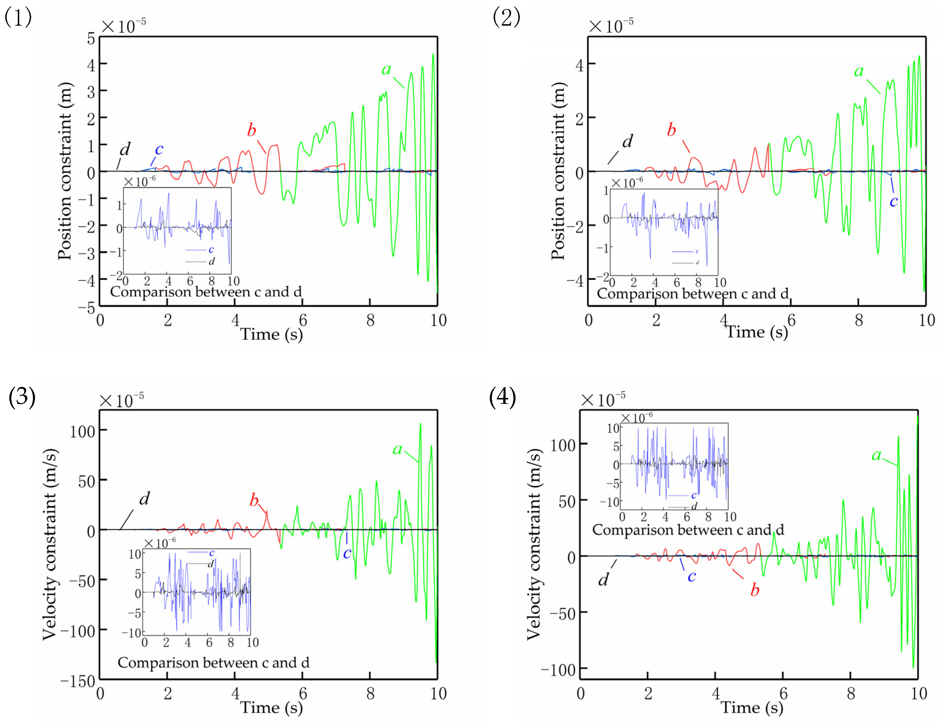
- (a)
- No constraint controls;
- (b)
- Direct elimination of position-level and velocity-level geometric constraint violations;
- (c)
- Simultaneous elimination of position-level and velocity-level geometric constraint violations;
- (d)
- Simultaneous elimination of position-level, velocity-level, and energy constraint violations.
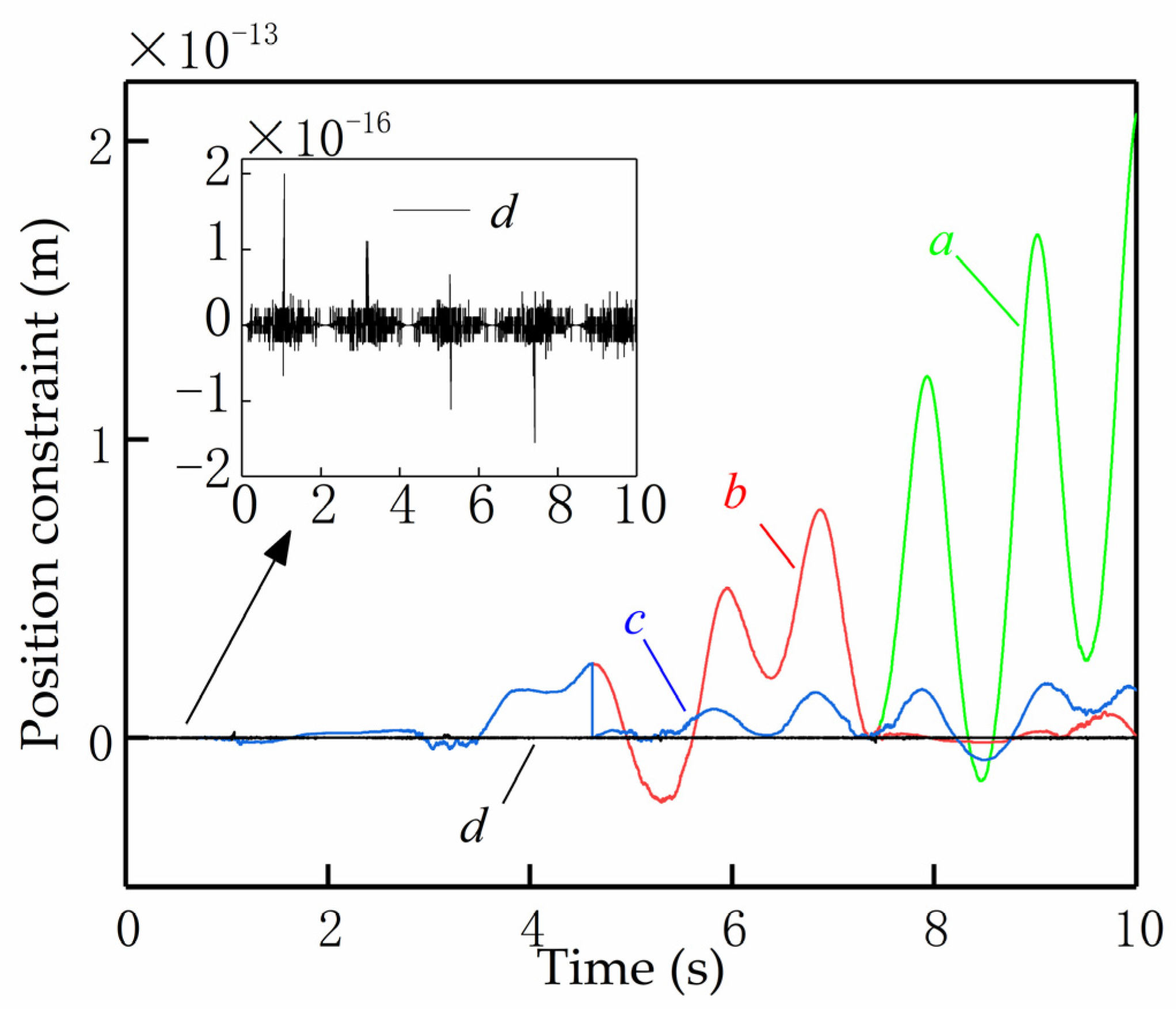
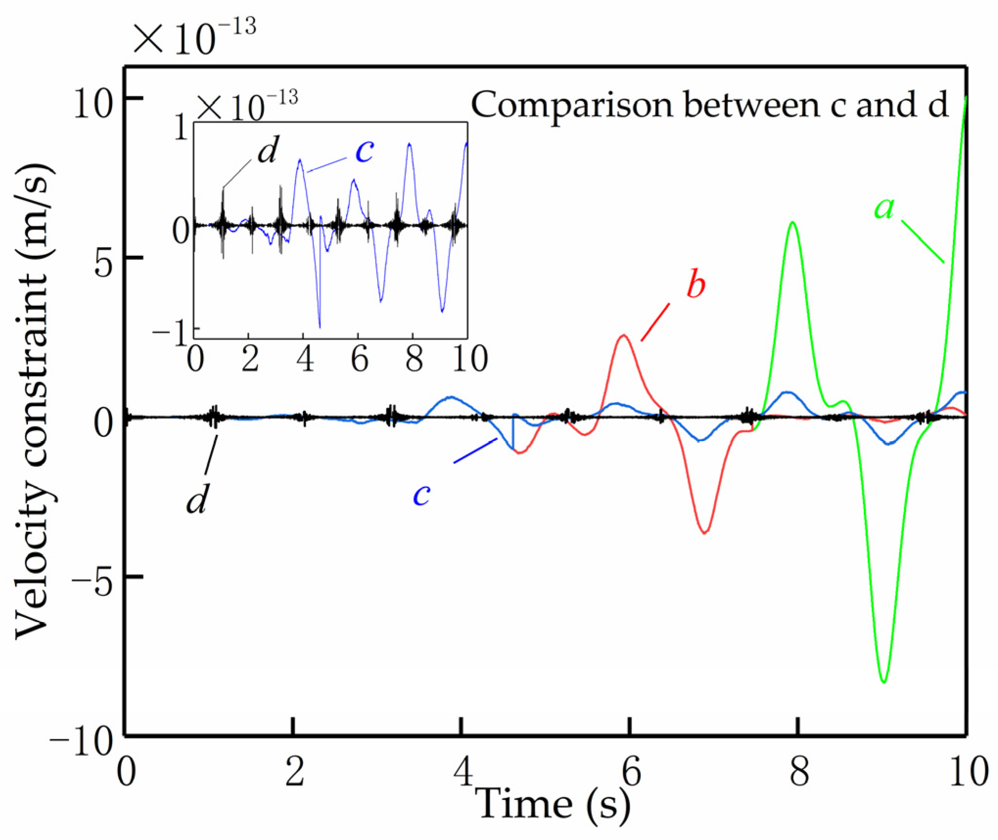

- (1)
- Position constraint violations in the x-direction;
- (2)
- Position constraint violations in the y-direction;
- (3)
- Velocity constraint violations in the x-directional;
- (4)
- Velocity constraint violations in the y-directional.
7. Conclusions
Author Contributions
Funding
Data Availability Statement
Conflicts of Interest
References
- Amirouche, F.M. Computational Methods in Multibody Dynamics; Prentice-Hall, Inc.: Englewood Cliffs, NJ, USA, 1992. [Google Scholar]
- De Jalon, J.G.; Bayo, E. Kinematic and Dynamic Simulation of Multibody Systems: The Real-Time Challenge; Springer Science & Business Media: Berlin, Germany, 2012. [Google Scholar]
- Liu, Y.; Pan, Z.; Ge, X. Dynamics of Multibody Systems; Higher Education Press: Beijing, China, 2014. [Google Scholar]
- Nikravesh, P.E. Computer-Aided Analysis of Mechanical Systems; Prentice-Hall, Inc.: Englewood Cliffs, NJ, USA, 1988. [Google Scholar]
- Roberson, R.E.; Schwertassek, R. Dynamics of Multibody Systems; Springer Science & Business Media: Berlin, Germany, 2012. [Google Scholar]
- Schiehlen, W. Multibody Systems Handbook; Springer: Berlin, Germany, 1990. [Google Scholar]
- Shabana, A.A. Dynamics of Multibody Systems; Cambridge University Press: Cambridge, UK, 2020. [Google Scholar]
- Wittenburg, J. Dynamics of Systems of Rigid Bodies; Springer: Berlin, Germany, 2013. [Google Scholar]
- Rulka, W. SIMPACK—A computer program for simulation of large-motion multibody systems. In Multibody Systems Handbook; Springer: Berlin/Heidelberg, Germany, 1990; pp. 265–284. [Google Scholar]
- Schupp, G.; Netter, H.; Mauer, L.; Gretzschel, M. Multibody system simulation of railway vehicles with SIMPACK. In The Manchester Benchmarks for Rail Vehicle Simulation; Routledge: London, UK, 2017; pp. 101–118. [Google Scholar]
- Rui, X.; Zhang, J.; Wang, X.; Rong, B.; He, B.; Jin, Z. Multibody system transfer matrix method: The past, the present, and the future. Int. J. Mech. Syst. Dyn. 2022, 2, 3–26. [Google Scholar] [CrossRef]
- Brandl, H.; Johanni, R.; Otter, M. A Very Efficient Algorithm for the Simulation of Robots and Similar Multibody Systems without Inversion of the Mass Matrix. IFAC Proc. Vol. 1986, 19, 95–100. [Google Scholar] [CrossRef]
- Cammarata, A.; Sinatra, R.; Maddìo, P.D. Interface reduction in flexible multibody systems using the Floating Frame of Reference Formulation. J. Sound Vib. 2022, 523, 116720. [Google Scholar] [CrossRef]
- Anderson, K.S. Recursive Derivation of Explicit Equations of Motion for Efficient Dynamic/Control Simulation of Large Multibody Systems; Stanford University: Stanford, CA, USA, 1990. [Google Scholar]
- Brandl, H. An Algorithm for the Simulation of Multibady An Algorithm for the Simulation of Multibody Systems with Kinematic Loops. In Proceedings of the 7th World Congress in the Theory of Machines and Mechanisms, Sevilla, Spain, 17–22 September 1987. [Google Scholar]
- Marques, F.; Souto, A.P.; Flores, P. On the constraints violation in forward dynamics of multibody systems. Multibody Syst. Dyn. 2017, 39, 385–419. [Google Scholar] [CrossRef] [Green Version]
- Nikravesh, P.E. Some Methods for Dynamic Analysis of Constrained Mechanical Systems: A Survey, Computer Aided Analysis and Optimization of Mechanical System Dynamics; Springer: Berlin, Germany, 1984; pp. 351–368. [Google Scholar]
- Baumgarte, J. Stabilization of constraints and integrals of motion in dynamical systems. Comput. Methods Appl. Mech. Eng. 1972, 1, 1–16. [Google Scholar] [CrossRef]
- Flores, P.; Machado, M.; Seabra, E.; Miguel, T. A Parametric Study on the Baumgarte Stabilization Method for Forward Dynamics of Constrained Multibody Systems. J. Comput. Nonlinear Dyn. 2009, 6, 011019. [Google Scholar] [CrossRef]
- Lin, S.-T.; Huang, J.-N. Stabilization of Baumgarte’s method using the Runge-Kutta approach. J. Mech. Des. 2002, 124, 633–641. [Google Scholar] [CrossRef] [Green Version]
- Zhang, P. A Stabilization of Constraints in the Numerical Solution of Euler-Lagrange Equation. Chin. J. Eng. Math. 2003, 20, 13–18. [Google Scholar]
- Carpinelli, M.; Gubitosa, M.; Mundo, D.; Desmet, W. Automated independent coordinates’ switching for the solution of stiff DAEs with the linearly implicit Euler method. Multibody Syst. Dyn. 2016, 36, 67–85. [Google Scholar] [CrossRef]
- Pappalardo, C.M.; Lettieri, A.; Guida, D. Stability analysis of rigid multibody mechanical systems with holonomic and nonholonomic constraints. Arch. Appl. Mech. 2020, 90, 1961–2005. [Google Scholar] [CrossRef]
- Wehage, K.T.; Wehage, R.A.; Ravani, B. Generalized coordinate partitioning for complex mechanisms based on kinematic substructuring. Mech. Mach. Theory 2015, 92, 464–483. [Google Scholar] [CrossRef]
- Fisette, P.; Vaneghem, B. Engineering, Numerical integration of multibody system dynamic equations using the coordinate partitioning method in an implicit Newmark scheme. Comput. Methods Appl. Mech. Eng. 1996, 135, 85–105. [Google Scholar] [CrossRef]
- Flores, P. A Study on Constraints Violation in Dynamic Analysis of Spatial Mechanisms. In Computational Kinematics; Zeghloul, S., Romdhane, L., Laribi, M., Eds.; Springer: Cham, Switzerland, 2018; pp. 593–601. [Google Scholar]
- Hong, J. Computational Multibody System Dynamics; Higher Education Press: Beijing, China, 1999. [Google Scholar]
- Yu, Q.; Chen, I.-M. A direct violation correction method in numerical simulation of constrained multibody systems. Comput. Mech. 2000, 26, 52–57. [Google Scholar]
- Bauchau, O.A.; Laulusa, A. Laulusa, Review of contemporary approaches for constraint enforcement in multibody systems. J. Comput. Nonlinear Dyn. 2008, 3, 011005. [Google Scholar] [CrossRef] [Green Version]
- Lyu, G.; Liu, R. Errors control of constraint violation in dynamical simulation for constrained mechanical systems. J. Comput. Nonlinear Dyn. 2019, 14, 031008. [Google Scholar]
- Xu, X.; Luo, J.; Wu, Z. Extending the modified inertia representation to constrained rigid multibody systems. J. Appl. Mech. 2020, 87, 011010. [Google Scholar] [CrossRef]
- Zhang, J.; Liu, D.; Liu, Y. A constraint violation suppressing formulation for spatial multibody dynamics with singular mass matrix. Multibody Syst. Dyn. 2016, 36, 87–110. [Google Scholar]
- Zhang, L.; Rui, X.; Zhang, J.; Gu, J.; Zheng, H.; Li, T. Study on Transfer Matrix Method for the Planar Multibody System with Closed-Loops. J. Comput. Nonlinear Dyn. 2021, 16, 121006. [Google Scholar] [CrossRef]
- Yoon, S.; Howe, R.M.; Greenwood, D.T. Geometric Elimination of Constraint Violations in Numerical Simulation of Lagrangian Equations. J. Mech. Des. 1994, 116, 1058–1064. [Google Scholar] [CrossRef]
- Eich, E. Convergence results for a coordinate projection method applied to mechanical systems with algebraic constraints. SIAM J. Numer. Anal. 1993, 30, 1467–1482. [Google Scholar] [CrossRef]
- Blajer, W. An orthonormal tangent space method for constrained multibody systems. Eng. Comput. Methods Appl. Mech. Eng. 1995, 121, 45–57. [Google Scholar] [CrossRef]
- Blajer, W. A geometric unification of constrained system dynamics. Multibody Syst. Dyn. 1997, 1, 3–21. [Google Scholar] [CrossRef]
- Blajer, W. Elimination of constraint violation and accuracy aspects in numerical simulation of multibody systems. Multibody Syst. Dyn. 2002, 7, 265–284. [Google Scholar] [CrossRef]
- Nikravesh, P.E. Initial condition correction in multibody dynamics. Multibody Syst. Dyn. 2007, 18, 107–115. [Google Scholar]
- Yoon, S.; Howe, R.M.; Greenwood, D.T. Constraint violation stabilization using gradient feedback in constrained dynamics simulation. J. Guid. Control. Dyn. 1992, 15, 1467–1474. [Google Scholar]
- García Orden, J.C. Energy considerations for the stabilization of constrained mechanical systems with velocity projection. Nonlinear Dyn. 2010, 60, 49–62. [Google Scholar]
- Garcia Orden, J.C.; Conde Martín, S. Controllable velocity projection for constraint stabilization in multibody dynamics. Nonlinear Dyn. 2012, 68, 245–257. [Google Scholar]
- Rui, X.; Bestle, D. Reduced multibody system transfer matrix method using decoupled hinge equations. Int. J. Mech. Syst. Dyn. 2021, 1, 182–193. [Google Scholar]


Disclaimer/Publisher’s Note: The statements, opinions and data contained in all publications are solely those of the individual author(s) and contributor(s) and not of MDPI and/or the editor(s). MDPI and/or the editor(s) disclaim responsibility for any injury to people or property resulting from any ideas, methods, instructions or products referred to in the content. |
© 2023 by the authors. Licensee MDPI, Basel, Switzerland. This article is an open access article distributed under the terms and conditions of the Creative Commons Attribution (CC BY) license (https://creativecommons.org/licenses/by/4.0/).
Share and Cite
Zhang, L.; Rui, X.; Zhang, J.; Gu, J.; Zhang, X. Exploring Energy in the Direct Correction Method for Correcting Geometric Constraint Violations. Mathematics 2023, 11, 1510. https://doi.org/10.3390/math11061510
Zhang L, Rui X, Zhang J, Gu J, Zhang X. Exploring Energy in the Direct Correction Method for Correcting Geometric Constraint Violations. Mathematics. 2023; 11(6):1510. https://doi.org/10.3390/math11061510
Chicago/Turabian StyleZhang, Lina, Xiaoting Rui, Jianshu Zhang, Junjie Gu, and Xizhe Zhang. 2023. "Exploring Energy in the Direct Correction Method for Correcting Geometric Constraint Violations" Mathematics 11, no. 6: 1510. https://doi.org/10.3390/math11061510