Estimation of Fixed Effects Partially Linear Varying Coefficient Panel Data Regression Model with Nonseparable Space-Time Filters

Abstract

Space-time panel data widely exist in many research fields such as economics, management, geography and environmental science. It is of interest to study the relationship between response variable and regressors which come from above fields by establishing regression models. This paper introduces a new fixed effects partially linear varying coefficient panel data regression model with nonseparable space-time filters. On the basis of approximating the varying coefficient functions with a powerful B-spline method, the profile quasi-maximum likelihood estimators of parameters and varying coefficient functions are constructed. Under some regular conditions, we derive their consistency and asymptotic normality. Monte Carlo simulation shows that our estimates have good finite performance and ignoring spatial and serial correlations may lead to inefficiency of estimates. Finally, the driving forces of Chinese resident consumption rate are studied using our estimation method.

1. Introduction

A space-time panel dataset is one sample collected from a number of spatial units over time periods (Li et al. [1]). Such datasets widely exist in economics, management, geography, environmental science and other research fields. How to effectively analyze space-time panel datasets and construct space-time panel data regression models has great theoretical and empirical significance. The space-time panel data regression models are a natural extension of panel data regression models. In the early 19th century, “regression” was first mentioned in the works of Legendre and Gauss. Later, at the turn of the 19th and 20th centuries, Galton and Pearson conceptualized regression, there were a number of regression models for analyzing panel data and exploring the association between dependent variable and regressors (Hsiao [2]; Baltagi [3]; Porter et al. [4]; Zamanzade [5]; Imai and Kim [6]). Among them, parametric panel data regression models have been widely used to study linear influence of regressors. Since the 1990s, nonparametric methods have been gradually applied into regression analysis (Fan and Gijbels [7]; Luo et al. [8]; Ullah et al. [9]; Dai et al. [10]), Li and Stengos [11] first proposed nonparametric panel data regression models to explore nonlinear influence of regressors. However, such models have their drawbacks. Parametric panel data regression models need to be precisely pre-specified, misspecified model forms can lead to inconsistent estimates as well as incorrect policy prescriptions. Although nonparametric panel data regression models are useful whenever we are not certain what the correct functional forms are, they may face the “curse of dimensionality” when the dimension of regressors is higher (Fan and Gijbels [7]), namely, the estimation accuracy decreases rapidly with the number of regressors increasing. Therefore, scholars proposed a number of non/semiparametric panel data regression models with a dimension reduction function to more flexibly overcome the “curse of dimensionality” encountered in practice, for example, partially linear additive panel data regression model, partially linear single-index panel data regression model and partially linear varying coefficient panel data regression model. In recent years, a series of their estimation methods have been also developed, including profile least squares estimation (Baltagi et al. [12]; Chen et al. [13]; Huang et al. [14]; Yong et al. [15]; Zhou et al. [16]; Zhang and Shen [17]), profile quasi-maximum likelihood estimation (Li et al. [18]; Su and Ullah [19]; Wu et al. [20]; Hu [21]), generalized method of moment estimation (GMM) (Tran and Tsionas [22]; Su and Ullah [23]), and others (Liu and Zhuang [24]).

All those modeling techniques and corresponding statistical inference methods for the above-mentioned semiparametric panel data regression models need the assumption that there is no correlation among the individuals or time periods. Elhorst [25] pointed out that two problems hampering the modeling of space-time panel data are serial correlation between the observations on each spatial unit over time and spatial correlation between the observations on the spatial units at each point in time. Furthermore, Baltagi et al. [12] mentioned that ignoring the serial correlation in the errors will result in consistent, but inefficient estimates of the regression coefficients and biased standard errors. Therefore, some scholars added nonseparable space-time filters, that is, space-time error correlation are modeled jointly, or separable space-time filters, that is, space-time error correlation are modeled independently from one another, under the framework of semi/parametric panel data regression models. The estimation, testing and empirical analysis of these models have been studied in recent years. Baltagi et al. [26] derived joint and conditional Lagrange Multiplier (LM) and Likelihood Ratio (LR) test statistics of random effects parametric panel regression model with separable space-time correlations and presented their small sample performance using Monte Carlo experiments. Elhorst [25] constructed a random effects parametric panel regression model with nonseparable space-time filters and presented its maximum likelihood estimation. Parent and LeSage [27] explored the Markov Chain Monte Carlo method of random effects parametric panel regression model with separable space-time filters—both Monte Carlo simulation and an application were used to illustrate the method. Lee and Yu [28] investigated quasi-maximum likelihood estimation for fixed effects parametric panel regression model with separable or nonseparable space-time filters, which might be spatially stable or unstable. They also derived consistency and asymptotic normality of the estimators under some regular conditions. Bai et al. [29] proposed a random effects partially linear varying coefficient panel model with separable space-time filters and derived consistency and asymptotic normality of weighted semiparametric least squares estimators. Zhao et al. [30] constructed weighted semiparametric least squares estimators and generalized F-type test statistic for random effects partially linear single-index panel model with separable space-time filters. They also derived the asymptotic properties of estimators and the asymptotic distribution of F-type test statistic. Li et al. [1] studied profile quasi-maximum likelihood estimation and generalized F-type test of random effects partially linear nonparametric panel model with separable space-time filters and obtained the consistency and asymptotic normality of parametric and nonparametric estimators as well as asymptotic distribution of generalized F-type test statistic. Monte Carlo simulation and Indonesian rice farming data were used to illustrate their methods.

To the best of our knowledge, there are no non/semiparametric spatiotemporal econometric models that study both fixed effects and nonseparable space-time filters in the existing literature. In this paper, we attempt to propose a fixed effects partially linear varying coefficient panel data regression model (PLVCPDRM) with nonseparable spacetime filters. It can simultaneously capture the linear and nonlinear effects of regressors, spatial and serial correlations of error structure, and individual fixed effects. Our aim is to construct profile quasi-maximum likelihood estimators (PQMLE) of this model and systematically study their asymptotic properties and finite sample performance. Furthermore, the proposed estimation method is illustrated by using a real dataset.

The rest of this paper is organized as follows: Section 2 presents a fixed effects PLVCPDRM with nonseparable space-time filters and its PQMLEs. Section 3 lays out some regular assumptions and asymptotic properties. Section 4 reports simulation results for examining the finite sample performance of the proposed estimators. Section 5 shows the empirical study for illustrating the proposed methodology. Conclusions are summarized in Section 6. Appendix A presents a lemma and proofs of the main theorems.

2. Model and Estimation

Consider a fixed effects PLVCPDRM with nonseparable space-time filters:

$$\begin{array}{cc}\hfill Y_{Nt}& =X_{Nt}\beta +Z_{\alpha ,Nt}+b+{\epsilon }_{Nt},t=1,\dots ,T,\hfill \end{array}$$

(1)

$$\begin{array}{cc}\hfill {\epsilon }_{Nt}& =\rho W{\epsilon }_{Nt}+\lambda {\epsilon }_{N,t-1}+e_{Nt},\hfill \end{array}$$

(2)

where $Y_{Nt}={(y_{1t},y_{2t},\dots ,y_{Nt})}^{\prime }$, $y_{it}$ are observations of a response variable, $i=1,\dots ,N$; $X_{Nt}={(x_{1t},x_{2t},\dots ,x_{Nt})}^{\prime }$, $Z_{\alpha ,Nt}={(z_{1t}^{\prime }\alpha \left(u_{1t}\right),\dots ,z_{Nt}^{\prime }\alpha \left(u_{Nt}\right))}^{\prime }$, $x_{it}={(x_{it1},x_{it2},\dots ,x_{itp})}^{\prime }$ and $z_{it}={(z_{it1},z_{it2},\dots ,z_{itq})}^{\prime }$ are observations of p-dimensional and q-dimensional exogenous regressors, respectively; $\beta$ is a regression coefficient vector of $x_{it}$, $\alpha \left(u_{it}\right)={({\alpha }_1\left(u_{it}\right),{\alpha }_2\left(u_{it}\right),\dots ,{\alpha }_q\left(u_{it}\right))}^{\prime }$ is an unknown univariate varying coefficient function vector, ${\alpha }_l\left(u\right)(l=1,\dots ,q)$ are smoothing functions of u, u is an intermediate univariate variable; $b={(b_1,\dots ,b_N)}^{\prime }$ are fixed effects satisfying ${\sum }_{i=1}^N{b}_i=0$ for identification purpose; W is an $N\times N$ row-normalized non-negative spatial weights matrix with zero diagonals; ${\epsilon }_{Nt}$ is an $N\times 1$ vector of disturbance term, $e_{Nt}$ is an $N\times 1$ vector of random error term which is assumed to be $i.i.d.(0,{\sigma }_e^2)$. In order to keep the stationarity of the model (1)–(2), serial correlation coefficient $\lambda$ and spatial correlation coefficient $\rho$ should belong to parameter space $\mathsf{\Theta }=\left\{\right(\lambda ,\rho ):\lambda +\rho <1,\lambda +\rho >-1,\lambda -\rho >-1,\lambda -\rho <1\}$ (Elhorst [25]; Lee and Yu [28]), see Figure 1.

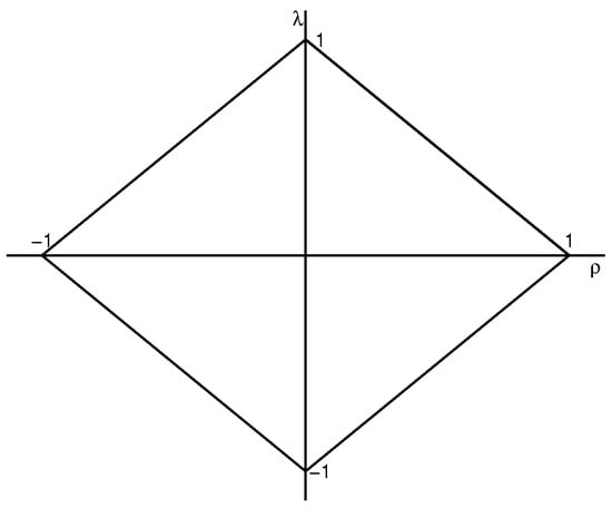
Figure 1. The parameter space $\mathsf{\Theta }$ of $\rho$ and $\lambda$.

For the model (1)–(2), it is necessary to identify an appropriate estimation method to obtain estimators of the unknown parameter vector $\theta ={({\beta }^{\prime },{\gamma }^{\prime },\rho ,\lambda ,{\sigma }_e^2)}^{\prime }$ and varying coefficient functions ${\alpha }_l(·)(l=1,\dots ,q)$.

Before proceeding to the estimation procedure, the fitting problem of the varying coefficient functions needs to be solved priority. Polynomial spline method is efficient in function approximation and numerical computation. Polynomial splines are piecewise polynomials with the polynomial pieces joining together smoothly at a set of interior knot points (see De Boor [31]; Huang and Shen [32]; Zou and Zhu [33]). B-spline is a special form of polynomial spline. Considering that the B-spline basis has better numerical properties than other basis functions, we use the B-spline method to approximate the varying coefficient functions ${\alpha }_l\left(u\right)(l=1,\dots ,q)$ in the model (1). To be precise, let $a=min\{u_{11},\dots ,u_{NT}\}$, $d=max\{u_{11},\dots ,u_{NT}\}$ and $a=$${\xi }_0<{\xi }_1<\dots <{\xi }_{k_l}=d(l=1,\dots ,q)$ be a partition of interval $[a,d]$. Using the ${\xi }_i$ as knots, we have ${\kappa }_l=k_l+k_0$ normalized B-spline basis function of order $(k_0-1)$ that forms a basis function for the linear spline space $S_{k_l}^{k_0}$ on $U=\left\{u_{it}\in \mathbb{R}\right\}$. Denote B-spline basis function ${\zeta }_l^{{\kappa }_l}\left(u\right)={({\zeta }_{l1}\left(u\right),\dots ,{\zeta }_{l{\kappa }_l}\left(u\right))}^{\prime }$, we can approximate ${\alpha }_l\left(u\right)$ by some spline function in $S_{k_l}^{k_0}$: ${\alpha }_l\left(u\right)\approx {\zeta }_l^{{\kappa }_l\prime }\left(u\right){\gamma }_l$, where ${\gamma }_l={({\gamma }_{l1},\dots ,{\gamma }_{l{\kappa }_l})}^{\prime }$ is an unknown ${\kappa }_l\times 1$ spline coefficient vector. Thus, the model (1) can be written as

$$Y_{Nt}=X_{Nt}\beta +{\tilde{Z}}_{Nt}\gamma +b+{\epsilon }_{Nt},$$

(3)

where $\gamma ={({\gamma }_1^{\prime },\dots ,{\gamma }_q^{\prime })}^{\prime }$, ${\tilde{Z}}_{Nt}={({\tilde{z}}_{1t},\dots ,{\tilde{z}}_{Nt})}^{\prime }$, ${\tilde{z}}_{it}^{\prime }=z_{it}^{\prime }{\zeta }_{q,K}\left(u_{it}\right)$ and

$${\zeta }_{q,K}\left(u\right)=\left(\begin{array}{ccccccccc}{\zeta }_{11}\left(u\right)& \dots & {\zeta }_{1{\kappa }_1}\left(u\right)& 0& \dots & 0& 0& \dots & 0\\ \dots & \dots & \dots & \dots & \dots & \dots & \dots & \dots & \dots \\ 0& \dots & 0& 0& \dots & 0& {\zeta }_{q1}\left(u\right)& \dots & {\zeta }_{q{\kappa }_q}\left(u\right)\end{array}\right)$$

is a $q\times K$ matrix, $K={\sum }_{s=1}^q{\kappa }_s$.

For any $N\times 1$ vector ${\mathbb{A}}_{Nt}$, denote $\Delta {\mathbb{A}}_{Nt}={\mathbb{A}}_{Nt}-{\mathbb{A}}_{N,t-1}$ as the first order difference. By first difference of the model (2)–(3) to eliminate the fixed effects, we have

$$\begin{array}{cc}\hfill & \Delta Y_{Nt}=\Delta X_{Nt}\beta +\Delta {\tilde{Z}}_{Nt}\gamma +\Delta {\epsilon }_{Nt},t=2,3,\dots ,T,\hfill \end{array}$$

(4)

$$\begin{array}{cc}\hfill & \Delta {\epsilon }_{Nt}=\rho W\Delta {\epsilon }_{Nt}+\lambda \Delta {\epsilon }_{N,t-1}+\Delta e_{Nt}.\hfill \end{array}$$

(5)

Note that $\Delta Y_{Nt}=Y_{Nt}-Y_{N,t-1}$ is observable for $t=2,3,\dots ,T$, $\Delta {\epsilon }_{N1}$ can’t be observed. Let $\eta ={(\rho ,\lambda )}^{\prime }$, $S_N\left(\rho \right)=I_N-\rho W$, $R_N\left(\lambda \right)=\lambda I_N$, $S_N=S\left({\rho }_0\right)$, $R_N=R\left({\lambda }_0\right)$ and $I_N$ is an $N\times N$ identity matrix. The Equation (5) can be rewritten as $S_N\left(\rho \right)\Delta {\epsilon }_{Nt}=$$R_N\left(\lambda \right)\Delta {\epsilon }_{N,t-1}+\Delta e_{Nt}$ for all t. With backward substitution, we have $S_N\left(\rho \right)\Delta {\epsilon }_{N,2}=$${\sum }_{j=0}^{\infty }{A}_N^j\left(\eta \right)\Delta e_{N,2-j}$, where $A_N\left(\eta \right)=R_N\left(\lambda \right)S_N{\left(\rho \right)}^{-1}$. By denoting $\Delta {\epsilon }_{N,T-1}={\left(\Delta {\epsilon }_{N2}^{\prime },\dots ,\Delta {\epsilon }_{NT}^{\prime }\right)}^{\prime }$ and

$$B_{N,T-1}\left(\eta \right)=\left(\begin{array}{ccccc}{S}_N\left(\rho \right)& \mathbf{0}& \dots & \mathbf{0}& \mathbf{0}\\ -R_N\left(\lambda \right)& S_N\left(\rho \right)& \dots & \mathbf{0}& \mathbf{0}\\ \mathbf{0}& -R_N\left(\lambda \right)& \dots & \mathbf{0}& \mathbf{0}\\ ⋮& ⋮& \ddots & \ddots & ⋮\\ \mathbf{0}& \mathbf{0}& \dots & -R_N\left(\lambda \right)& S_N\left(\rho \right)\end{array}\right),$$

the matrix form of the Equation (5) can be simply expressed as $B_{N,T-1}\left(\eta \right)\Delta {\epsilon }_{N,T-1}=({(S_N\left(\rho \right)\Delta {\epsilon }_{N2})}^{\prime }$, $\Delta e_{N3}^{\prime },\dots ,\Delta e_{NT}^{\prime }{)}^{\prime }$. As $Var\left[{\sum }_{j=0}^{\infty }{A}_N^j\left(\eta \right)\Delta e_{N,2-j}\right]={\sigma }_e^2{K}_N\left(\eta \right)$, where

$$K_N\left(\eta \right)\equiv I_N+\sum _{j=0}^{\infty }{A}^j\left(\eta \right)\left(A_N\left(\eta \right)-I_N\right){\left(A_N\left(\eta \right)-I_N\right)}^{\prime }{A}_N^{\prime j}\left(\eta \right),$$

and $K_N=K_N\left({\eta }_0\right)$, we can obtain $Var(B_{N,T-1}\left(\eta \right)\Delta {\epsilon }_{N,T-1})={\sigma }_e^2{\mathsf{\Omega }}_{N,T-1}\left(\eta \right)$ with

$${\mathsf{\Omega }}_{N,T-1}\left(\eta \right)=\left(\begin{array}{cccccc}{K}_N\left(\eta \right)& -I_N& \mathbf{0}& \dots & \mathbf{0}& \mathbf{0}\\ -I_N& 2I_N& -I_N& \dots & \mathbf{0}& \mathbf{0}\\ \mathbf{0}& -I_N& 2I_N& \dots & \mathbf{0}& \mathbf{0}\\ ⋮& ⋮& ⋮& \ddots & ⋮& ⋮\\ \mathbf{0}& \mathbf{0}& \mathbf{0}& \dots & 2I_N& -I_N\\ \mathbf{0}& \mathbf{0}& \mathbf{0}& \dots & -I_N& 2I_N\end{array}\right).$$

Note that the only unknown element of ${\mathsf{\Omega }}_{N,T-1}\left(\eta \right)$ is $K_N\left(\eta \right)$. In order to obtain determinant and inverse of ${\mathsf{\Omega }}_{N,T-1}\left(\eta \right)$, we define a confirmable block matrix (Hsiao et al [34]; Lee and Yu [28]) as

$$P_{N,T-1}\left(\eta \right)=\left(\begin{array}{ccccc}{I}_N& \mathbf{0}& \mathbf{0}& \dots & \mathbf{0}\\ I_N& K_N\left(\eta \right)& \mathbf{0}& \dots & \mathbf{0}\\ I_N& K_N\left(\eta \right)& 2K_N\left(\eta \right)-I_N& \dots & \mathbf{0}\\ ⋮& ⋮& ⋮& \ddots & ⋮\\ I_N& K_N\left(\eta \right)& 2K_N\left(\eta \right)-I_N& \dots & (T-2)K_N\left(\eta \right)-(T-3)I_N\end{array}\right).$$

From straight calculation, we know that

$$\begin{array}{cc}\hfill D_{N,T-1}\left(\eta \right)& \equiv P_{N,T-1}\left(\eta \right){\mathsf{\Omega }}_{N,T-1}\left(\eta \right)P_{N,T-1}^{\prime }\left(\eta \right)\hfill \\ \hfill & =diag\left\{K_N\left(\eta \right),\left(2K_N\left(\eta \right)-I_N\right)K_N\left(\eta \right),\left(3K_N\left(\eta \right)-2I_N\right)\left(2K_N\left(\eta \right)-I_N\right),\dots ,\right.\hfill \\ \hfill & \left.\left[(T-1)K_N\left(\eta \right)-(T-2)I_N\right]\left[(T-2)K_N\left(\eta \right)-(T-3)I_N\right]\right\}.\hfill \end{array}$$

Thus, the determinant $|{\mathsf{\Omega }}_{N,T-1}\left(\eta \right)|=|D_{N,T-1}\left(\eta \right)|/|P_{N,T-1}{\left(\eta \right)|}^2=|(T-1)K_N\left(\eta \right)-(T-2)I_N|$ and the inverse ${\mathsf{\Omega }}_{N,T-1}^{-1}\left(\eta \right)=P_{N,T-1}{\left(\eta \right)}^{\prime }{D}_{N,T-1}{\left(\eta \right)}^{-1}{P}_{N,T-1}\left(\eta \right)$. Therefore, the quasi-log-likelihood function can be written as

$$\begin{array}{cc}\hfill log{L}_{N,T}\left(\theta \right)=& -\frac{N(T-1)}{2}log\left(2\pi {\sigma }_e^2\right)-\frac{1}{2}log\left|I_N+(T-1)(K_N\left(\eta \right)-I_N)\right|\hfill \\ \hfill & +(T-1)log\left|S_N\left(\rho \right)\right|-\frac{1}{2{\sigma }_e^2}{\left[Y-X\beta -\tilde{Z}\gamma \right]}^{\prime }{\mathbb{J}}_{NT}\left(\eta \right)\left[Y-X\beta -\tilde{Z}\gamma \right],\hfill \end{array}$$

(6)

where $Y={(Y_{N1}^{\prime },\dots ,Y_{NT}^{\prime })}^{\prime }$, $X={(X_{N1}^{\prime },\dots ,X_{NT}^{\prime })}^{\prime }$, $\tilde{Z}={({\tilde{z}}_{11},\dots ,{\tilde{z}}_{NT})}^{\prime }$, ${\mathbb{J}}_{NT}\left(\eta \right)=L_{N,(T-1)T}^{\prime }$$B_{N,T-1}^{\prime }\left(\eta \right){\mathsf{\Omega }}_{N,T-1}^{-1}\left(\eta \right)B_{N,T-1}\left(\eta \right)L_{N,(T-1)T}$, $L_{N,(T-1)T}=L\otimes I_N$ with

$$L=\left(\begin{array}{ccccc}-1& 1& 0& \dots & 0\\ 0& -1& 1& \dots & 0\\ ⋮& ⋮& ⋮& \ddots & 0\\ 0& 0& 0& -1& 1\end{array}\right)$$

as the first order difference transformation matrix of dimension $(T-1)\times T$.

Motivated by Su and Jin [35], we obtain PQMLEs of parameter vector $\theta$ and varying coefficient functions ${\alpha }_l(·)(l=1,\dots ,q)$ by the following the two-step estimation procedure:

Step 1: Assuming the parameter $\eta$ is known, the initial estimators of ${({\beta }^{\prime },{\gamma }^{\prime },{\sigma }_e^2)}^{\prime }$ can be obtained by maximizing quasi-log-likelihood function (6):

$${\widehat{\beta }}_{IN}={\left[X^{\prime }{\mathbb{J}}_{NT}\left(\eta \right)X\right]}^{-1}{X}^{\prime }{\mathbb{J}}_{NT}\left(\eta \right)\left[Y-\tilde{Z}{\widehat{\gamma }}_{IN}\right],$$

$${\widehat{\gamma }}_{IN}={\left[{\tilde{Z}}^{\prime }{\mathbb{J}}_{NT}\left(\eta \right)\tilde{Z}\right]}^{-1}{\tilde{Z}}^{\prime }{\mathbb{J}}_{NT}\left(\eta \right)\left[Y-X{\widehat{\beta }}_{IN}\right],$$

$${\widehat{\sigma }}_{eIN}^2=\frac{1}{N(T-1)}{\left[Y-X{\widehat{\beta }}_{IN}-\tilde{Z}{\widehat{\gamma }}_{IN}\right]}^{\prime }{\mathbb{J}}_{NT}\left(\eta \right)\left[Y-X{\widehat{\beta }}_{IN}-\tilde{Z}{\widehat{\gamma }}_{IN}\right].$$

Step 2: With the estimated ${\widehat{\beta }}_{IN}$, ${\widehat{\gamma }}_{IN}$ and ${\widehat{\sigma }}_{eIN}^2$, PQMLE of $\eta$ can be obtained by maximizing the concentrated quasi-log-likelihood function of $\eta$:

$$\begin{array}{cc}\hfill log{L}_{N,T}\left(\eta \right)=& -\frac{N(T-1)}{2}log\left(2\pi \right)-\frac{N(T-1)}{2}(log{\widehat{\sigma }}_{eIN}^2+1)\hfill \\ \hfill & -\frac{1}{2}log\left|I_N+(T-1)(K_N\left(\eta \right)-I_N)\right|+(T-1)log\left|S_N\left(\rho \right)\right|.\hfill \end{array}$$

The final estimator of $\eta$ is given by $\widehat{\eta }=arg{max}_{\eta }log{L}_{N,T}\left(\eta \right)$. With the estimated $\widehat{\eta }$, update

${\widehat{\beta }}_{IN}^{\prime },{\widehat{\gamma }}_{IN}^{\prime }$ and ${\widehat{\sigma }}_{eIN}^2$, we can obtain the final PQMLEs as

$$\widehat{\beta }={\left[X^{\prime }{(I-{\mathbb{S}}_{\widehat{\eta }})}^{\prime }{\mathbb{J}}_{NT}\left(\widehat{\eta }\right)(I-{\mathbb{S}}_{\widehat{\eta }})X\right]}^{-1}{X}^{\prime }{(I-{\mathbb{S}}_{\widehat{\eta }})}^{\prime }{\mathbb{J}}_{NT}\left(\widehat{\eta }\right)(I-{\mathbb{S}}_{\widehat{\eta }})Y,$$

$$\widehat{\gamma }={\left[{\tilde{Z}}^{\prime }{\mathbb{J}}_{NT}\left(\widehat{\eta }\right)\tilde{Z}\right]}^{-1}{\tilde{Z}}^{\prime }{\mathbb{J}}_{NT}\left(\widehat{\eta }\right)\left[Y-X\widehat{\beta }\right],$$

(7)

$${\widehat{\sigma }}_e^2=\frac{1}{N(T-1)}{\left[Y-X\widehat{\beta }\right]}^{\prime }{(I-{\mathbb{S}}_{\widehat{\eta }})}^{\prime }{\mathbb{J}}_{NT}\left(\widehat{\eta }\right)(I-{\mathbb{S}}_{\widehat{\eta }})\left[Y-X\widehat{\beta }\right],$$

where I is an identity matrix of dimension $NT$, ${\mathbb{S}}_{\eta }=\tilde{Z}{\left[{\tilde{Z}}^{\prime }{\mathbb{J}}_{NT}\left(\eta \right)\tilde{Z}\right]}^{-1}{\tilde{Z}}^{\prime }{\mathbb{J}}_{NT}\left(\eta \right)$. Then, the estimator of the nonparametric function $\alpha \left(u\right)$ can be written as

$$\widehat{\alpha }\left(u\right)={\zeta }_{q,K}\left(u\right)\widehat{\gamma }.$$

(8)

3. Asymptotic Properties

To derive the asymptotic properties of the estimators, we first introduce some regular assumptions. For clear exposition, denote ${\theta }_0={({\beta }_0^{\prime },{\gamma }_0^{\prime },{\eta }_0^{\prime },{\sigma }_{e0}^2)}^{\prime }$, ${\theta }_0^{*}={({\beta }_0^{\prime },{\eta }_0^{\prime },{\sigma }_{e0}^2)}^{\prime }$ and ${\eta }_0={({\rho }_0,{\lambda }_0)}^{\prime }$ as the true parameter vector of $\theta$, ${\theta }^{*}$ and $\eta$, respectively, and ${\alpha }_0\left(u\right)$ as the true varying coefficient function vector of $\alpha \left(u\right)$.

Assumption 1.

(i) The sequences ${\left\{x_{it}\right\}}_{i=1,t=1}^{N,T}$, ${\left\{z_{it}\right\}}_{i=1,t=1}^{N,T}$ and ${\left\{u_{it}\right\}}_{i=1,t=1}^{N,T}$ are nonstochastic, and they have bounded support set on ${\mathbb{R}}^p$, ${\mathbb{R}}^q$ and ${\mathbb{R}}^1$ respectively. In addition, $u_{it}$ forms a sequence of designs such that they are analogous to a positive and bounded “design density“ $f_U\left(u\right)$ (Su and Jin [35]).

(ii) For any bounded continuous function  $h(·)$, it holds that

$$\underset{N\to \infty }{lim}\frac{1}{NT}\sum _{i=1}^N\sum _{t=1}^{T}h(u_{it})={\int }_{U}h\left(u\right)f_U\left(u\right)du.$$

(9)

(iii) The parameter $\beta \in {\mathbb{R}}^p$ in a neighborhood of ${\beta }_0$ satisfies $|x_{it}^{\prime }\beta |\le m_x$, where $m_x$ is a positive constant.

Assumption 2.

The disturbances ${\left\{e_{it}\right\}}_{i=1,t=2}^{N,T}$ are $i.i.d.$ with zero mean, variance ${\sigma }_{e0}^2$ and $E{\left|e_{it}\right|}^{4+ϵ}<\infty$ for some $ϵ>0$.

Assumption 3.

(i) For every K, the smallest eigenvalue of ${\tilde{Z}}^{\prime }\tilde{Z}/NT$ and ${\tilde{Z}}^{\prime }{\mathbb{J}}_{NT}\left({\eta }_0\right)\tilde{Z}/NT$ are bounded away from zero uniformly in K.

(ii) There is a sequence of constants ${\zeta }_0\left(K\right)$ satisfying ${sup}_{u\in U}∥{\zeta }_{q,K}\left(u\right)∥\le {\zeta }_0\left(K\right)$ such that ${\zeta }_0^2\left(K\right)K/N$$\to 0$ as $N\to \infty$.

(iii) For any $r_1$-th$(r_1\ge 2)$ continuously differentiable bounded function $\alpha (·)$ satisfying the normalization of ${\alpha }_0(·)$, there exist some $r_2>0$ such that ${sup}_{u\in U}\left|z_{it}^{\prime }\alpha \left(u_{it}\right)-{\tilde{z}}_{it}^{\prime }\gamma \right|=O\left(K^{-r_2}\right)$ as $K\to \infty$ and $\sqrt{N}{K}^{-r_2}\to 0$ as $N\to \infty$.

Assumption 4.

(i) W is a row-normalized and prespecified spatial weights matrix.

(ii) Row and column sums of W in absolute value are uniformly bounded (i.e., UB).

(iii) $S_N\left(\rho \right)$ is invertible for all $\rho \in \mathbb{P}$, where $\mathbb{P}$ is compact and the true parameter ${\rho }_0$ is in the interior of $\mathbb{P}$. Additionally, $S_N^{-1}\left(\rho \right)$ is UB for $\rho \in \mathbb{P}$.

Assumption 5.

(i) ${\sum }_{h=1}^{\infty }abs\left(A_N^h\right)$ is UB, where ${\left[abs\left(A_N\right)\right]}_{ij}=\left|A_{N,ij}\right|$ and $A_N=A_N\left({\eta }_0\right)$.

(ii) ${\mathbb{J}}_{NT}\left(\eta \right)$ is UB.

(iii) The limit of the information matrix (A4) in Appendix A is nonsingular.

(iv) ${lim}_{N\to \infty }\frac{1}{N(T-1)}{[X,\tilde{Z}]}^{\prime }{\mathbb{J}}_{NT}\left(\eta \right)[X,\tilde{Z}]$ is nonsingular.

Assumption 6.

${lim}_{N\to \infty }{T}_{NT,1}\left(\eta ,{\sigma }_e^2\right)\ne 0$ for ${\left(\eta ,{\sigma }_e^2\right)}^{\prime }\ne {\left({\eta }_0,{\sigma }_{e0}^2\right)}^{\prime }$, where $T_{NT,1}$ is defined in (A1).

Remark 1.

The fixed bounded design in Assumption 1 is typically assumed in spatial econometric literature, see Kelejian and Prucha [36], Kelejian and Prucha [37], Su and Jin [35] and Cheng and Chen [38]. Assumption 1 (ii) parallels Assumption 1 of Su and Jin [35] and Assumption 2.1 (iv) of Hu et al. [39]. It means that if ${\left\{u_{it}\right\}}_{i=1,t=1}^{N,T}$ are $i.i.d.$ with the density $f_U(·)$, the Equation (9) holds with probability 1. Assumption 2 presents regularity assumptions for error terms $e_{it}$. Assumption 3 is a set of mild conditions on the B-spline method (see Newey [40]; Hu et al. [39]; Yong et al. [15]; Zhang [41]). Assumption 3(i) ensures that ${\tilde{Z}}^{\prime }\tilde{Z}$ and ${\tilde{Z}}^{\prime }{\mathbb{J}}_{NT}\left({\eta }_0\right)\tilde{Z}$ are asymptotically nonsingular, which parallels Assumption 3 of Zhang [41] and Assumption 2(i) of Newey [40]. Newey [40] gave some primitive conditions for power series and splines such that Assumption 3(ii)–(iii) hold. In addition, Assumption 3(iii) is the counterpart assumption in the kernel method. Assumption 4 provides the basic features of the spatial weight matrix. The uniform boundedness of W and $S_N^{-1}\left(\rho \right)$ limits the spatial correlation to a manageable degree in Assumptions 4(ii)–(iii). Assumption 5(i) is the absolute summability condition and row/column sum boundedness condition for disturbances, which will play an important role for the proofs of asymptotic properties. To prove the absolute summability of $A_N$, a sufficient condition is $∥A_N∥<1$ for any matrix norm (see Corollary 5.6.16 in Horn and Johnson [42]) that satisfies $∥A_N∥=∥abs\left(A_N\right)∥$. When $∥A_N∥<1$, ${\sum }_{h=0}^{\infty }{A}_N^h$ exists and can be defined as ${\left(I_N-A_N\right)}^{-1}$. Under the condition that the inverse of the variance matrix of ${(1-\varphi )}^{1/2}{e}_{Nt}+\left(A_N-I_N\right)\left(e_{N,t-1}+A_N{e}_{N,t-2}+A_N^2{e}_{N,t-3}+\dots \right)$ is UB for $\varphi =0,1$ and $\frac{T-2}{T-1}$, Assumption 5(ii) can be certified. Assumption 5(iii)–(iv) is used for establishing the uniqueness identification and asymptotic normality of the proposed estimators. Assumption 6 specifies an identification condition for the estimators of parameters when Assumption 5(iv) is not satisfied.

In order to prove consistency of the parametric estimators, we need to obtain the expected value function for the quasi-log-likelihood function (6) divided by the effective sample size $N(T-1)$. The relationship $B_{NT}^{*}\epsilon =e$ between $\epsilon ={({\epsilon }_{N1}^{\prime },\dots ,{\epsilon }_{NT}^{\prime })}^{\prime }$ and $e={(e_{N1}^{†\prime },\dots ,e_{NT}^{\prime })}^{\prime }$ (the first block of N in e are not exactly the original $e_{N1}$ and all the entries are i.i.d. under normality) would be used frequently, where

$$B_{NT}^{*}={\left(\begin{array}{ccccc}{Q}_N^{*}& \mathbf{0}& \dots & \mathbf{0}& \mathbf{0}\\ -R_N& S_N& \dots & \mathbf{0}& \mathbf{0}\\ \mathbf{0}& -R_N& \dots & \mathbf{0}& \mathbf{0}\\ ⋮& ⋮& \ddots & \ddots & ⋮\\ \mathbf{0}& \mathbf{0}& \dots & -R_N& S_N\end{array}\right)}_{NT\times NT}$$

and $Q_N^{*}={\left({\sum }_{j=0}^{\infty }{A}_N^j{A}_N^{j\prime }\right)}^{-1/2}{S}_N$. Thus, $e_{N1}^{†}=Q_N^{*}{S}_N^{-1}$${\sum }_{j=0}^{\infty }{A}_N^j{e}_{N,1-j}$ and $Q_N^{*}Var\left({\epsilon }_{N1}\right)Q_N^{*\prime }={\sigma }_{e0}^2{I}_N$ under the normality of disturbances. Split $B_{NT}^{*}$ into four block matrices, one of which is $Q_N^{*}$. Utilizing the formula ${\left(\begin{array}{cc}A& \mathbf{0}\hfill \\ B& C\hfill \end{array}\right)}^{-1}=\left(\begin{array}{cc}{A}^{-1}& \mathbf{0}\\ -C^{-1}B{A}^{-1}& C^{-1}\end{array}\right)$ for inversion of a block matrix, we have that

$$B_{NT}^{*-1}=\left(\begin{array}{ccccccc}{Q}_N^{*-1}& & & & & & \\ A_N{Q}_N^{*-1}& S_N^{-1}& & & & \\ A_N^2{Q}_N^{*-1}& A_N{S}_N^{-1}& S_N^{-1}& & & & \\ ⋮& ⋮& ⋮& \ddots & & & \\ ⋮& ⋮& ⋮& \ddots & \ddots & & \\ A_N^{T-1}{Q}_N^{*-1}& A_N^{T-2}{S}_N^{-1}& A_N^{T-3}{S}_N^{-1}& \dots & \dots & A_N{S}_N^{-1}& S_N^{-1}\end{array}\right).$$

Define $Q_{N,T}\left(\theta \right)=\mathrm{E}(log{L}_{N,T}\left(\theta \right)/N(T-1))$, then

$$\begin{array}{cc}\hfill Q_{N,T}\left(\theta \right)=& -\frac{1}{2}log\left(2\pi {\sigma }_e^2\right)+\frac{1}{N}log\left|S\left(\rho \right)\right|-\frac{1}{2N(T-1)}log\left|I_N+(T-1)(K_N-I_N)\right|\hfill \\ \hfill & -\frac{1}{2{\sigma }_e^{2}N(T-1)}{e}^{\prime }{B}_{NT}^{*-1\prime }{\mathbb{J}}_{NT}\left(\eta \right)B_{NT}^{*-1}e.\hfill \end{array}$$

(10)

However, when $e^{†}={(e_{N1}^{†\prime },\dots ,e_{NT}^{\prime })}^{\prime }$ are not normally distributed, elements in $e_{N1}^{†}$ are uncorrelated but not necessarily independent of each other even though they are independent with $e_{Nt}$($t=2,\dots ,T$). Consider the case that the process starts at a finite past period, such as $t=-m$. Denote $e_{N,T+m}={(e_{N,1-m}^{\prime },e_{N,1-(m-1)}^{\prime },\dots ,e_{N0}^{\prime },e_{N1}^{\prime },\dots ,e_{NT}^{\prime })}^{\prime }$, which includes the original $i.i.d.$ disturbances vectors, we have $e^{†}=F_{NT,N(T+m)}{e}_{N,T+m}$, where

$$\begin{array}{cc}\hfill & F_{NT,N(T+m)}\hfill \\ \hfill =& \left(\begin{array}{ccccccc}{\left(\sum _{j=0}^m{A}_N^j{A}_N^{j\prime }\right)}^{-\frac{1}{2}}·A_N^m& \dots & {\left(\sum _{j=0}^m{A}_N^j{A}_N^{j\prime }\right)}^{-\frac{1}{2}}·A_N& {\left(\sum _{j=0}^m{A}_N^j{A}_N^{j\prime }\right)}^{-\frac{1}{2}}·I_N& & & \\ & & & & I_N& & \\ & & & & & \ddots \\ & & & & & & I_N\end{array}\right)\hfill \end{array}$$

is UB. Under non-normality, we can obtain

$$\begin{array}{cc}\hfill Q_{N,T}\left(\theta \right)=& -\frac{1}{2}log\left(2\pi {\sigma }_e^2\right)+\frac{1}{N}log\left|S\left(\rho \right)\right|-\frac{1}{2N(T-1)}log\left|I_N+(T-1)(K_N-I_N)\right|\hfill \\ \hfill & -\frac{1}{2{\sigma }_e^{2}N(T-1)}{e}_{N,T+m}^{\prime }{F}_{NT,N(T+m)}^{\prime }{B}_{NT}^{*-1\prime }{\mathbb{J}}_{NT}\left(\eta \right)B_{NT}^{*-1}{F}_{NT,N(T+m)}{e}_{N,T+m}.\hfill \end{array}$$

(11)

To show the consistency of $\widehat{\theta }$, we follow Lee [43] by identifying ${\theta }_0$ based upon the maximum value of $Q_{N,T}\left(\theta \right)$ and showing the uniform convergence of $\frac{1}{N(T-1)}log{L}_{N,T}\left(\theta \right)-Q_{N,T}\left(\theta \right)$ to zero, consistency of $\widehat{\theta }$ follows.

Theorem 1.

Suppose Assumptions 1–6 hold, ${\theta }_0$ is globally identifiable and $\widehat{\theta }$ is consistent with ${\theta }_0$.

Theorem 2.

Suppose Assumptions 1–6 hold, as $N\to \infty$ simultaneously, we have

$$\sqrt{NT}\left({\widehat{\theta }}^{*}-{\theta }_0^{*}\right)\stackrel{L}{\to }\mathrm{N}\left(0,{\mathsf{\Sigma }}_{{\theta }_0^{*}}^{-1}+{\mathsf{\Sigma }}_{{\theta }_0^{*}}^{-1}{\mathsf{\Omega }}_{{\theta }_0^{*}}{\mathsf{\Sigma }}_{{\theta }_0^{*}}^{-1}\right).$$

where “$\stackrel{L}{\to }$” means convergence in distribution, ${\mathsf{\Sigma }}_{{\theta }_0^{*}}=-\underset{N,T\to \infty }{lim}E\left(\frac{1}{N(T-1)}\frac{{\partial }^{2}log{L}_{N,T}\left({\theta }_0^{*}\right)}{\partial {\theta }^{*}\partial {\theta }^{*\prime }}\right)$ is an expected Hessian matrix showed in (A5) and $E\left(\frac{1}{N(T-1)}\frac{\partial log{L}_{N,T}\left({\theta }_0^{*}\right)}{\partial {\theta }^{*}}\frac{\partial log{L}_{N,T}\left({\theta }_0^{*}\right)}{\partial {\theta }^{*\prime }}\right)={\mathsf{\Sigma }}_{{\theta }_0^{*}}+{\mathsf{\Omega }}_{{\theta }_0^{*}}+o_P\left(1\right)$ with ${\mathsf{\Omega }}_{{\theta }_0^{*}}$ defined in (A6).

Theorem 3.

Suppose Assumptions 1–5 hold, we have

$$\left|\widehat{\alpha }\left(u_{it}\right)-{\widehat{\alpha }}_0\left(u_{it}\right)\right|=O_P\left({\zeta }_0\left(K\right)(\sqrt{K}/\sqrt{N}+K^{-r_2})\right).$$

Remark 2.

The term $K/N$ essentially corresponds to a variance term and $K^{-2r_2}$ to a bias term. When K is chosen as $N^{\frac{1}{1+2r_2}}$ so that these two terms go to zero at the same rate, which occurs when K goes to infinity at the same rate as $N^{\frac{1}{1+2r_2}}$ (and the side condition ${\zeta }_0{\left(K\right)}^{2}K/N\to 0$ is satisfied), the convergence rate will be $N^{-\frac{r_2}{1+2r_2}}$.

Theorem 4.

Suppose Assumptions 1–5 hold, as $N\to \infty$ simultaneously, we have

$${\mathsf{\Lambda }}_u^{-1/2}\left(\widehat{\alpha }\left(u\right)-{\alpha }^{*}\left(u\right)\right)\stackrel{L}{⟶}\mathrm{N}(0,{\sigma }_{e0}^2{I}_K),$$

where ${\mathsf{\Lambda }}_u={\zeta }_{q,K}\left(u\right){[{\tilde{Z}}^{\prime }{\mathbb{J}}_{NT}\left({\eta }_0\right)\tilde{Z}]}^{-1}{\tilde{Z}}^{\prime }{\mathbb{J}}_{NT}\left({\eta }_0\right)B_{NT}^{*-1}{B}_{NT}^{*\prime -1}$${\mathbb{J}}_{NT}^{\prime }\left({\eta }_0\right)\tilde{Z}{[{\tilde{Z}}^{\prime }{\mathbb{J}}_{NT}\left({\eta }_0\right)\tilde{Z}]}^{-1}{\zeta }_{q,K}^{\prime }\left(u\right)$, ${\alpha }^{*}\left(u\right)={\zeta }_{q,K}\left(u\right){\gamma }_0$, $I_K$ is an identity matrix of dimension K.

4. Simulation Studies

In this section, we report the results of Monte Carlo simulation experiments to examine the finite sample performance of the proposed estimation method. In order to illustrate the estimation accuracy of parameters, we use the sample mean (Mean), the sample standard deviation (SD) and the root mean square error (RMSE) as the evaluation criteria. Here,

$$RMSE={\left(\frac{1}{mcn}\sum _{i=1}^{mcn}{\left({\widehat{\theta }}_i-{\theta }_0\right)}^2\right)}^{\frac{1}{2}},$$

where $mcn$ is the simulation times, ${\widehat{\theta }}_i(i=1,2,\dots ,mcn)$ are the parametric estimates of each simulation and ${\theta }_0$ is the true value. For the nonparametric estimates, we consider the mean absolute deviation error (MADE) as the evaluation criterion which is defined as

$${MADE}_j=Q^{-1}\sum _{q=1}^Q\left|{\widehat{g}}_j\left(u_q\right)-g_j\left(u_q\right)\right|,j=1,2,\dots ,mcn,$$

where ${\left\{u_q\right\}}_{q=1}^Q$ are Q fixed grid points at support set of u.

Example 1.

The first example is to evaluate the performance of the estimation procedure. Consider the following data-generated processes:

$$\{\begin{array}{c}{y}_{it}=x_{it1}{\beta }_1+x_{it2}{\beta }_2+z_{it1}{\alpha }_1\left(u_{it}\right)+z_{it2}{\alpha }_2\left(u_{it}\right)+b_i+{\epsilon }_{it},\hfill \\ {\epsilon }_{it}=\rho {\displaystyle \sum _{j=1}^N}{w}_{ij}{\epsilon }_{jt}+\lambda {\epsilon }_{i,t-1}+e_{it},\hfill \end{array}$$

(12)

where $x_{itp}\sim \mathrm{U}[-2,2](p=1,2)$, $z_{itq}\sim \mathrm{U}[-2,2](q=1,2)$, $u_{it}\sim \mathrm{U}[-3,3]$, $b_i\sim i.i.d.\mathrm{N}(0,1)$, $e_{it}\sim i.i.d.\mathrm{N}(0,0.5)$, the link functions ${\alpha }_1\left(u_{it}\right)=0.5u_{it}+sin\left(1.5u_{it}\right)$ and ${\alpha }_2\left(u_{it}\right)=u_{it}^2+0.5u_{it}$, $\left({\beta }_1,{\beta }_2\right)=(1,1.5)$. As in Su [44], the spatial weighting matrix is set to the Rook weight matrix. Sample size is $T=10,15,20$ and $N=25,49,81$. For each case, we ran 500 simulations. The R software was used.

Table 1 summarizes Means, Medians, SDs and RMSEs for parametric estimates of ${\widehat{\beta }}_1,{\widehat{\beta }}_2,\widehat{\rho },\widehat{\lambda }$ and ${\widehat{\sigma }}_e^2$ when the true values of spatial correlation coefficient and serial correlation coefficient are set as $(\rho ,\lambda )=(0.4,0.4),(0.2,0.7)$ and $(0.7,0.2)$, respectively. Table 2 and Table 3 give the median and SD of MADE values of ${\widehat{\alpha }}_1\left(u\right)$ and ${\widehat{\alpha }}_2\left(u\right)$ at 20 fixed grid points in all cases, respectively. We have the following finds: (1) The estimates of ${\beta }_1,{\beta }_2,\rho ,\lambda ,{\sigma }_e^2$ are close to true values for all cases; (2) SDs and RMSEs for ${\widehat{\beta }}_1,{\widehat{\beta }}_2,\widehat{\rho },\widehat{\lambda },{\widehat{\sigma }}_e^2$ are fairly small for all cases; (3) For fixed T(or N), as N(or T) increased, the SDs and RMSEs for estimates of all parameters decrease; (4) The SDs and Medians for 500 MADEs of ${\widehat{\alpha }}_1\left(u\right)$ and ${\widehat{\alpha }}_2\left(u\right)$ at 20 fixed grid points decrease as T or N is increased. Based on these findings, we conclude that the estimates of all parameters and varying coefficient functions are fairly close to their true values, and the deviations decrease with increasing of sample size. Overall, our proposed estimators for the model (12) perform well in finite sample cases.

Table 1. Simulation results of parametric estimates ${\widehat{\beta }}_1,{\widehat{\beta }}_2,\widehat{\rho },\widehat{\lambda }$ and ${\widehat{\sigma }}_e^2$.

			T = 10			T = 15			T = 20
N	Parameter	$(\mathit{\rho },\mathit{\lambda })$	$(0.2,0.7)$	$(0.4,0.4)$	$(0.7,0.2)$	$(0.2,0.7)$	$(0.4,0.4)$	$(0.7,0.2)$	$(0.2,0.7)$	$(0.4,0.4)$	$(0.7,0.2)$
25	${\beta }_1$	Mean	0.9998	0.9993	0.9990	0.9994	0.9978	0.9968	0.9999	0.9998	0.9999
		Median	0.9985	0.9962	1.0002	1.0004	0.9987	0.9989	1.0002	1.0003	1.0003
		SD	0.0344	0.0391	0.0399	0.0277	0.0310	0.0309	0.0235	0.0261	0.0259
		RMSE	0.0344	0.0390	0.0398	0.0277	0.0310	0.0310	0.0235	0.0260	0.0259
	${\beta }_2$	Mean	1.4971	1.4972	1.4963	1.4976	1.4978	1.4983	1.5015	1.5011	1.5004
		Median	1.4970	1.4940	1.4960	1.4984	1.4978	1.4975	1.5018	1.5017	1.5007
		SD	0.0357	0.0394	0.0380	0.0273	0.0300	0.0296	0.0231	0.0257	0.0257
		RMSE	0.0357	0.0395	0.0381	0.0273	0.0300	0.0296	0.0231	0.0257	0.0257
	$\rho$	Mean	0.2513	0.4282	0.7199	0.2354	0.4139	0.7103	0.2303	0.4125	0.7089
		Median	0.2489	0.4335	0.7214	0.2385	0.4162	0.7130	0.2317	0.4115	0.7060
		SD	0.0948	0.0640	0.0396	0.0713	0.0465	0.0279	0.0601	0.0417	0.0236
		RMSE	0.1076	0.0698	0.0443	0.0795	0.0484	0.0297	0.0671	0.0435	0.0252
	$\lambda$	Mean	0.7598	0.4237	0.2022	0.7423	0.4153	0.2029	0.7339	0.4091	0.1984
		Median	0.7625	0.4368	0.1995	0.7484	0.4101	0.1965	0.7339	0.4054	0.2000
		SD	0.0921	0.0955	0.0592	0.0723	0.0616	0.0409	0.0626	0.0526	0.0316
		RMSE	0.1096	0.0982	0.0591	0.0837	0.0633	0.0410	0.0711	0.0533	0.0316
	${\sigma }_e^2$	Mean	0.4196	0.4020	0.3950	0.4483	0.4366	0.4334	0.4608	0.4507	0.4473
		Median	0.4172	0.4139	0.3944	0.4490	0.4388	0.4368	0.4606	0.4501	0.4496
		SD	0.0438	0.0443	0.0470	0.0385	0.0361	0.0383	0.0349	0.0313	0.0328
		RMSE	0.0915	0.1075	0.1149	0.0644	0.0729	0.0768	0.0524	0.0584	0.0621
49	${\beta }_1$	Mean	1.0005	1.0012	1.0017	0.9984	0.9984	0.9994	0.9993	0.9991	1.0006
		Median	0.9994	1.0026	1.0036	0.9991	0.9998	0.9980	1.0003	0.9989	0.9999
		SD	0.0267	0.0293	0.0286	0.0185	0.0207	0.0209	0.0176	0.0195	0.0175
		RMSE	0.0267	0.0293	0.0286	0.0185	0.0207	0.0209	0.0176	0.0194	0.0175
	${\beta }_2$	Mean	1.5010	1.5006	1.5002	1.5014	1.5011	1.5008	1.4982	1.4977	1.5027
		Median	1.5009	1.4944	1.5011	1.5009	1.5015	1.5022	1.4981	1.4970	1.5007
		SD	0.0264	0.0290	0.0283	0.0187	0.0204	0.0215	0.0159	0.0179	0.0181
		RMSE	0.0264	0.0290	0.0283	0.0187	0.0204	0.0216	0.0159	0.0180	0.0181
	$\rho$	Mean	0.2545	0.4213	0.7109	0.2456	0.4135	0.7064	0.2347	0.4042	0.7059
		Median	0.2538	0.4209	0.7133	0.2446	0.4110	0.7079	0.2297	0.4023	0.7064
		SD	0.0728	0.0466	0.0321	0.0645	0.0403	0.0233	0.0556	0.0282	0.0168
		RMSE	0.0908	0.0512	0.0338	0.0789	0.0424	0.0241	0.0655	0.0285	0.0177
	$\lambda$	Mean	0.7540	0.4207	0.2089	0.7482	0.4079	0.1997	0.7410	0.4066	0.1961
		Median	0.7533	0.4122	0.1995	0.7446	0.3983	0.1944	0.7468	0.4042	0.1959
		SD	0.0780	0.0847	0.0512	0.0661	0.0481	0.0353	0.0570	0.0388	0.0272
		RMSE	0.0947	0.0900	0.0519	0.0817	0.0486	0.0354	0.0701	0.0393	0.0275
	${\sigma }_e^2$	Mean	0.4412	0.4291	0.4238	0.4680	0.4526	0.4481	0.4759	0.4650	0.4582
		Median	0.4378	0.4205	0.4179	0.4649	0.4536	0.4452	0.4714	0.4614	0.4590
		SD	0.0378	0.0350	0.0393	0.0319	0.0277	0.0311	0.0290	0.0261	0.0252
		RMSE	0.0692	0.0790	0.0857	0.0551	0.0549	0.0605	0.0417	0.0436	0.0488
81	${\beta }_1$	Mean	1.0013	1.0016	1.0018	0.9995	0.9996	1.0000	1.0001	1.0001	0.9997
		Median	1.0004	1.0029	1.0036	1.0002	0.9999	1.0003	1.0002	1.0003	1.0003
		SD	0.0205	0.0223	0.0216	0.0156	0.0175	0.0175	0.0126	0.0146	0.0145
		RMSE	0.0205	0.0223	0.0216	0.0156	0.0175	0.0175	0.0126	0.0146	0.0145
	${\beta }_2$	Mean	1.5012	1.5017	1.5019	1.4996	1.4993	1.4991	1.5002	1.5006	1.5005
		Median	1.5023	1.5023	1.5022	1.5000	1.5007	1.5009	1.5009	1.5014	1.5007
		SD	0.0197	0.0219	0.0215	0.0147	0.0160	0.0158	0.0127	0.0141	0.0139
		RMSE	0.0197	0.0219	0.0215	0.0147	0.0160	0.0157	0.0127	0.0141	0.0139
	$\rho$	Mean	0.2654	0.4161	0.7087	0.2489	0.4096	0.7049	0.2463	0.4072	0.7042
		Median	0.2458	0.4184	0.7099	0.2497	0.4079	0.7058	0.2455	0.4071	0.7060
		SD	0.0624	0.0333	0.0252	0.0522	0.0259	0.0163	0.0492	0.0214	0.0161
		RMSE	0.0767	0.0370	0.0266	0.0714	0.0276	0.0170	0.0551	0.0225	0.0166
	$\lambda$	Mean	0.7556	0.4190	0.2088	0.7519	0.4076	0.2016	0.7427	0.4044	0.2013
		Median	0.7505	0.4002	0.2006	0.7507	0.4025	0.1973	0.7453	0.4037	0.2000
		SD	0.0723	0.0688	0.0442	0.0531	0.0425	0.0274	0.0443	0.0289	0.0231
		RMSE	0.0911	0.0712	0.0450	0.0742	0.0430	0.0274	0.0598	0.0292	0.0231
	${\sigma }_e^2$	Mean	0.4518	0.4362	0.4340	0.4724	0.4577	0.4565	0.4779	0.4654	0.4649
		Median	0.4485	0.4333	0.4287	0.4726	0.4570	0.4558	0.4753	0.4656	0.4650
		SD	0.0366	0.0305	0.0338	0.0254	0.0223	0.0236	0.0202	0.0174	0.0220
		RMSE	0.0604	0.0707	0.0742	0.0475	0.0478	0.0495	0.0335	0.0387	0.0414

Table 2. The Medians and SDs of MADE values for ${\widehat{\alpha }}_1\left(u\right)$.

		T = 10			T = 15			T = 20
$(\mathit{\rho },\mathit{\lambda })$		N = 25	N = 49	N = 81	N = 25	N = 49	N = 81	N = 25	N = 49	N = 81
(0.2, 0.7)	Median	0.0782	0.0553	0.0443	0.0622	0.0426	0.0347	0.0553	0.0405	0.0310
	SD	0.0203	0.0148	0.0113	0.0174	0.0105	0.0096	0.0157	0.0101	0.0080
(0.4, 0.4)	Median	0.0853	0.0604	0.0488	0.0693	0.0473	0.0379	0.0628	0.0445	0.0337
	SD	0.0219	0.0159	0.0121	0.0193	0.0116	0.0110	0.0177	0.0112	0.0092
(0.7, 0.2)	Median	0.0835	0.0588	0.0495	0.0670	0.0491	0.0383	0.0627	0.0424	0.0334
	SD	0.0217	0.0150	0.0117	0.0187	0.0128	0.0108	0.0177	0.0107	0.0090

Table 3. The Medians and SDs of MADE values for ${\widehat{\alpha }}_2\left(u\right)$.

		T = 10			T = 15			T = 20
$(\mathit{\rho },\mathit{\lambda })$		N = 25	N = 49	N = 81	N = 25	N = 49	N = 81	N = 25	N = 49	N = 81
(0.2, 0.7)	Median	0.0776	0.0532	0.0444	0.0683	0.0442	0.0350	0.0563	0.0378	0.0306
	SD	0.0213	0.0152	0.0115	0.0183	0.0115	0.0091	0.0143	0.0112	0.0078
(0.4, 0.4)	Median	0.0856	0.0599	0.0480	0.0672	0.0498	0.0384	0.0618	0.0426	0.0336
	SD	0.0231	0.0166	0.0125	0.0198	0.0128	0.0099	0.0153	0.0123	0.0088
(0.7, 0.2)	Median	0.0846	0.0606	0.0476	0.0653	0.0460	0.0375	0.0607	0.0413	0.0329
	SD	0.0226	0.0159	0.0129	0.0191	0.0113	0.0097	0.0153	0.0115	0.0090

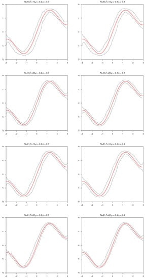
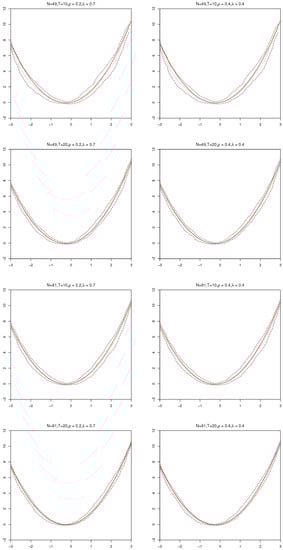
Figure 2 and Figure 3 present the fitting results and 95% confidence intervals of ${\alpha }_1\left(u\right)$ and ${\alpha }_2\left(u\right)$ under $N=49$ (or 81) and $T=15$ (or 20), where the short dashed curves in black are the average fits over 500 simulations by PQMLE, the solid curves in red are the true values of nonparametric functions and the two long dashed curves in black are the corresponding 95% confidence bands. We can see that the short dashed curve is close to the solid curve, and the confidence bandwidth gradually becomes narrow with the increase of the sample size. They indicate that the nonparametric estimation procedure is feasible in the case of small samples.

Figure 2. The fitting results and 95% confidence intervals of ${\alpha }_1\left(u\right)$ in the model (12).

Figure 3. The fitting results and 95% confidence intervals of ${\alpha }_2\left(u\right)$ in the model (12).

Example 2.

The second example is used to show that misspecification for the model (12) will lead to inconsistent parameter estimates. Here are the three most likely misspecified models, which ignore the spatial correlation, serial correlation and spatio-temporal correlations in the model (12), respectively:

$$\{\begin{array}{c}{y}_{it}=x_{it1}{\beta }_1+x_{it2}{\beta }_2+z_{it1}{\alpha }_1\left(u_{it}\right)+z_{it2}{\alpha }_2\left(u_{it}\right)+b_i+{\epsilon }_{it},\hfill \\ {\epsilon }_{it}=\lambda {\epsilon }_{i,t-1}+e_{it},\hfill \end{array}$$

(13)

$$\{\begin{array}{c}{y}_{it}=x_{it1}{\beta }_1+x_{it2}{\beta }_2+z_{it1}{\alpha }_1\left(u_{it}\right)+z_{it2}{\alpha }_2\left(u_{it}\right)+b_i+{\epsilon }_{it},\hfill \\ {\epsilon }_{it}=\rho {\displaystyle \sum _{j=1}^N}{w}_{ij}{\epsilon }_{jt}+e_{it},\hfill \end{array}$$

(14)

$$y_{it}=x_{it1}{\beta }_1+x_{it2}{\beta }_2+z_{it1}{\alpha }_1\left(u_{it}\right)+z_{it2}{\alpha }_2\left(u_{it}\right)+b_i+e_{it},$$

(15)

where all variables in the above models are the same as the model (12). No loss of generality, we only study the case that $\rho =0.4$ and $\lambda =0.4$. Additionally, we set $N=25,49$, $T=10$ and $mcn=500$. The experimental results are presented in Table 4.

Table 4. Simulation results of parametric estimates for the models (12)–(15).

		N = 25,T = 10					N = 49,T = 10
Model		${\mathit{\beta }}_1$	${\mathit{\beta }}_2$	$\mathit{\rho }$	$\mathit{\lambda }$	${\mathit{\sigma }}_{\mathit{e}}^2$	${\mathit{\beta }}_1$	${\mathit{\beta }}_2$	$\mathit{\rho }$	$\mathit{\lambda }$	${\mathit{\sigma }}_{\mathit{e}}^2$
Model (12)	Mean	1.9993	1.4972	0.4282	0.4237	0.4020	1.0012	1.5006	0.4213	0.4207	0.4291
	Median	0.9962	1.4940	0.4335	0.4368	0.4139	1.0016	1.4944	0.4209	0.4122	0.4205
	SD	0.0391	0.0394	0.0640	0.0955	0.0443	0.0293	0.0290	0.0466	0.0847	0.0350
	RMSE	0.0390	0.0395	0.0698	0.0982	0.1075	0.0293	0.0290	0.0512	0.0900	0.0790
Model (13)	Mean	0.9989	1.4996	-	0.5610	0.5508	1.0011	1.5012	-	0.5456	0.5735
	Median	0.9981	1.4985	-	0.5649	0.5485	1.0026	1.4924	-	0.5689	0.5778
	SD	0.0429	0.0464	-	0.1066	0.0671	0.0324	0.0328	-	0.0694	0.0499
	RMSE	0.0428	0.0463	-	0.1930	0.0841	0.0324	0.0328	-	0.1612	0.0888
	MR	97.4%	17.21%	-	96.54%	−21.77%	10.58%	13.10%	-	79.11%	12.41%
Model (14)	Mean	0.9984	1.4956	0.4145	-	0.4145	1.0009	1.5003	0.4542	-	0.4410
	Median	0.9961	1.4939	0.4667	-	0.4139	1.0006	1.5003	0.4567	-	0.4379
	SD	0.0440	0.0426	0.0670	-	0.0499	0.0310	0.0328	0.0448	-	0.0351
	RMSE	0.0439	0.0427	0.0942	-	0.0989	0.0310	0.0328	0.0703	-	0.0686
	MR	12.56%	8.10%	34.96%	-	−8.00%	5.80%	13.10%	37.30%	-	−13.16%
Model (15)	Mean	0.9969	1.4991	-	-	0.6073	1.0000	1.5007	-	-	0.6309
	Median	0.9964	1.4982	-	-	0.5955	0.9987	1.5032	-	-	0.6278
	SD	0.0550	0.0544	-	-	0.0953	0.0368	0.0408	-	-	0.0677
	RMSE	0.0549	0.0543	-	-	0.1434	0.0367	0.0407	-	-	0.1473
	MR	40.76%	37.46%	-	-	33.39%	25.25%	40.34%	-	-	86.45%

Note: True values ( ${\beta }_{10}$, ${\beta }_{20}$, ${\sigma }_{e0}^2$)′ = (1, 1.5, 0.5)′ for the models (12)–(15), λ₀ = 0.4 for the model (13) and ρ₀ = 0.4 for the model (14).

Table 4 lists the Means, Medians, SDs, RMSEs and MRs of parameter estimates in the models (12)–(15), where MR is the growth rate of RMSE on the basis of that in the model (12). From Table 4, we can see that: (1) The Means and Medians for the estimates of all parameters in the model (12) are closer to true values as sample size increases. However, it is easy to see that the Means and Medians of ${\widehat{\beta }}_1$, ${\widehat{\beta }}_2$, $\widehat{\rho }$, $\widehat{\lambda }$ and ${\widehat{\sigma }}_e^2$ in the models (13)–(15) do not converge with the increasing of N, indicating that they are not stable. (2) The SDs and RMSEs of almost all parameter estimators in the models (13)–(15) are larger than that in the model (12). In particular, the SDs and RMSEs of ${\widehat{\sigma }}_e^2$ do not decrease with the increasing of sample size. (3) MRs of most parameter estimators are greater than 0% and increase with the increasing of sample size, especially for ${\widehat{\beta }}_2$, $\widehat{\rho }$ and ${\widehat{\sigma }}_e^2$. In addition, MRs of ${\widehat{\sigma }}_e^2$ in the models (13) and (14) are less than 0%, which again indicates that the estimator of ${\sigma }_e^2$ is unstable. It can be concluded that model misspecification would result in inconsistent parameter estimators. It further indicates that our proposed model is more effective and reliable.

5. Real Data Analysis

In this section, we employ the proposed model and its estimation method to study the driving forces of Chinese resident consumption rate. This dataset was collected on 1 August 2022) from the China Statistical Yearbook (http://www.stats.gov.cn/sj/ndsj/) for 2008 to 2020 and covers 30 provincial administrative regions (except Tibet, Taiwan, Hong Kong and Macau). Based on the research results drawn by Ding and Chen [45] and Ding [46], let $YC$ be response variable and $LR$, $CR$, $ER$, $GR$ and $TR$ be regressors. There is no doubt that per capita disposable income has an important impact on the resident consumption rate. Therefore, we assume that the impacts of the above regressors on resident consumption rate may be realized through per capita disposable income and $IR$ is selected as their intermediate variable. The definitions of these variables and their meanings are given in Table 5.

Table 5. Variable definitions and their meanings.

Response Variable	Definition
$YC$	The ratio of resident consumption to GDP
Regressors	Definition
$LR$	The ratio of the population over 65 to the population between 14 and 65
$CR$	The ratio of the population under 14 to the population between 14 and 65
$ER$	The ratio of the population with junior college degree or above to total population
$GR$	The ratio of the male population to total population
$TR$	The ratio of the tertiary industry to GDP
Intermediate Variable	Definition
$IR$	Growth rate of per capita disposable income

Firstly, Table 6 and Figure 4 show the descriptive statistics of the response variable, five regressors and intermediate variable. From observing Table 6, we can draw the conclusion that $LR$, $CR$, $ER$, $GR$, $TR$ and $IR$ are steady, as well as concluding that $GR$ has a small fluctuation range. In addition, Figure 4 presents the scatter plots between $YC$ versus each regressor ($LR$, $CR$, $ER$, $GR$ and $TR$). It can be found that the regressor $LR$ has a linear effect on the response variable $YC$. The rest of the regressors have nonlinear effects on the response variable $YC$.

Table 6. The descriptive statistics of the response variable, five regressors and intermediate variable.

	Min	1st Qu.	Median	Mean	3rd Qu.	Max	SD	Range
$YC$	0.2160	0.3260	0.3609	0.3642	0.4001	0.5811	0.0579	0.3651
$LR$	0.0744	0.1132	0.1361	0.1407	0.1612	0.2548	0.0351	0.1804
$CR$	0.0965	0.1791	0.2311	0.2289	0.2767	0.3981	0.0639	0.3016
$ER$	0.0285	0.0806	0.1063	0.1219	0.1398	0.4769	0.0698	0.4484
$GR$	0.4873	0.5057	0.5108	0.5117	0.5168	0.5519	0.0091	0.0645
$TR$	0.2830	0.3875	0.4461	0.4581	0.5100	0.8400	0.0990	0.5570
$IR$	−0.0285	0.0795	0.0890	0.0946	0.1162	0.2038	0.0355	0.2323

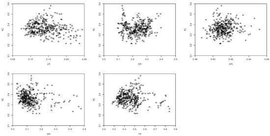
Figure 4. Scatter plots of the response variable versus five regressors, respectively.

Based on the above comprehensive analysis, the study on driving forces of Chinese resident consumption rate can be analyzed by establishing the following PLVCPDRM with nonseparable space-time filters:

$$\begin{array}{cc}\hfill Y{C}_{it}& =L{R}_{it}\beta +C{R}_{it}{\alpha }_1\left(I{R}_{it}\right)+E{R}_{it}{\alpha }_2\left(I{R}_{it}\right)+G{R}_{it}{\alpha }_3\left(I{R}_{it}\right)+T{R}_{it}{\alpha }_4\left(I{R}_{it}\right)+b_i+{\epsilon }_{it}\hfill \\ \hfill {\epsilon }_{it}& =\rho \sum _{j=1}^N{w}_{ij}{\epsilon }_{jt}+\lambda {\epsilon }_{i,t-1}+e_{it},i=1,\dots ,30,t=1,\dots ,13,\hfill \end{array}$$

(16)

where $W={\left(w_{ij}\right)}_{30\times 30}$ is a normalized spatial weight matrix calculated by the Euclidean distance in the light of the longitude and latitude coordinates of any two provinces.

Table 7 reports the estimation results of parameters in the model (16). It can be seen that $\widehat{\rho }=0.6126$ and $\widehat{\lambda }=0.3674$ are significant. Namely, it indicates that there exist strong and positive spatial and serial correlations among the disturbance terms in the model (16). Furthermore, $\widehat{\beta }=-0.1751<0$ is significant, which means that the linear effect of $LR$ on the resident consumption rate is negative. Figure 5 shows the varying coefficient effects of $CR$, $ER$, $GR$ and $TR$ to $YC$ and their $95\%$ confidence intervals. It can be seen that $CR$, $ER$, $GR$ and $TR$ have obvious nonlinear effects on resident consumption rate with $IR$.

Table 7. Estimation results of parameters in the model (16).

	$\mathit{\beta }$	$\mathit{\rho }$	$\mathit{\lambda }$	${\mathit{\sigma }}_{\mathit{e}}^2$
Estimator	−0.1751 ***	0.6126 ***	0.3674 ***	0.0005 ***
SD	0.1072	0.1432	0.0329	9.6963 × 10${}^{-5}$

Notes: *** represents that the regressor is significant under the significance level 1%.

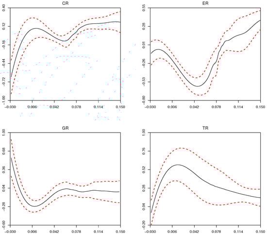
Figure 5. Varying coefficient effects of $CR$, $ER$, $GR$ and $TR$ to $YC$ and their $95\%$ confidence intervals, respectively.

6. Concluding Remarks

In order to sufficiently use the information of spatial and serial correlations in the disturbances when modeling space-time data by regression models, we propose a fixed effects PLVCPDRM with nonseparable space-time filters. It can not only simultaneously capture non/linear effects of regressors and space-time correlations of error structure, but also overcome the “curse of dimensionality” in multivariate nonparametric regression models.

In this paper, the PQMLEs of unknown parameters and varying coefficient functions for this model are constructed. Under the regular assumptions, we prove that the estimators satisfy consistency and asymptotic normality. Monte Carlo simulations show that the proposed estimators have good finite sample performances. In addition, ignoring spatial and serial correlations in errors of the model would result in inconsistent and inefficient estimators. Finally, a Chinese resident consumption rate dataset is used to illustrate our estimation method.

This paper mainly focuses on the estimation of a fixed effects PLVCPDRM with nonseparable space-time filters. In the future, we may study the methods of variable selection, Bayesian estimation and quantile regression for the proposed model in our paper; we can also use the proposed method to study similar semiparametric panel data regression models with space-time filters.

References

- Li, S.; Chen, J.; Li, B. Estimation and testing of random effects semiparametric regression model with separable space-time filters. Fractal Fract. 2022, 6, 735. [Google Scholar] [CrossRef]
- Hsiao, C. Benefits and limitations of panel data. Economet. Rev. 1985, 4, 121–174. [Google Scholar] [CrossRef]
- Baltagi, B.H. Panel data methods. In Handbook of Applied Economic Statistics; CRC Press: Boca Raton, FL, USA, 1998; pp. 311–323. [Google Scholar]
- Porter, C.O.; Outlaw, R.; Gale, J.P.; Cho, T.S. The use of online panel data in management research: A review and recommendations. J. Manag. 2019, 45, 319–344. [Google Scholar] [CrossRef]
- Zamanzade, E. EDF-based tests of exponentiality in pair ranked set sampling. Stat. Pap. 2019, 60, 2141–2159. [Google Scholar] [CrossRef]
- Imai, K.; Kim, I.S. On the use of two-way fixed effects regression models for causal inference with panel data. Polit. Anal. 2021, 29, 405–415. [Google Scholar] [CrossRef]
- Fan, J.; Gijbels, I. Local Polynomial Modelling and Its Applications; Chapman and Hall: London, UK, 1996. [Google Scholar]
- Luo, G.; Wu, M.; Pang, Z. Empirical likelihood inference for the semiparametric varying-coefficient spatial autoregressive model. J. Syst. Sci. Complex. 2021, 34, 2310–2333. [Google Scholar] [CrossRef]
- Ullah, A.; Wang, T.; Yao, W. Semiparametric partially linear varying coefficient modal regression. J. Econom. 2022. [Google Scholar] [CrossRef]
- Dai, X.; Li, S.; Jin, L.; Tian, M. Quantile regression for partially linear varying coefficient spatial autoregressive models. Commun. Stat-Simul. 2022, 1–16. [Google Scholar] [CrossRef]
- Li, Q.; Stengos, T. Semiparametric estimation of partially linear panel data models. J. Econom. 1996, 71, 389–397. [Google Scholar] [CrossRef]
- Baltagi, B.H.; Li, D. Series estimation of partially linear panel data models with fixed effects. Ann. Econ. Financ. 2002, 3, 103–116. [Google Scholar]
- Chen, J.; Gao, J.; Li, D. Estimation in partially linear single-index panel data models with fixed effects. J. Bus. Econ. Stat. 2013, 31, 315–330. [Google Scholar] [CrossRef]
- Huang, B.; Sun, Y.; Wang, S. Estimation of partially linear panel data models with cross-sectional dependence. J. Syst. Sci. Complex. 2021, 34, 2219–2230. [Google Scholar] [CrossRef]
- Yong, A.; Cheng, H.; Dong, L. Semiparametric estimation of partially linear varying coefficient panel data models. Adv. Econom. 2016, 36, 47–65. [Google Scholar]
- Zhou, B.; You, J.; Xu, Q.; Chen, G. Weighted profile least squares estimation for a panel data varying-coefficient partially linear model. Chin. Ann. Math. B 2010, 31, 247–272. [Google Scholar] [CrossRef]
- Zhang, Y.; Shen, D. Estimation of semi-parametric varying-coefficient spatial panel data models with random-effects. J. Stat. Plan. Infer. 2015, 159, 64–80. [Google Scholar] [CrossRef]
- Li, S.; Chen, J.; Chen, D. PQMLE of a partially linear varying coefficient spatial autoregressive panel model with random effects. Symmetry 2021, 13, 2057. [Google Scholar] [CrossRef]
- Su, L.; Ullah, A. Profile likelihood estimation of partially linear panel data models with fixed effects. Econ. Lett. 2006, 92, 75–81. [Google Scholar] [CrossRef]
- Wu, Q.; Luo, X.; Li, Y. Partially linear varying-coefficient panel data models with fixed effects. Far East J. Theor. Stat. 2008, 25, 229–238. [Google Scholar]
- Hu, X. Estimation in a semi-varying coefficient model for panel data with fixed effects. J. Syst. Sci. Complex. 2014, 27, 594–604. [Google Scholar] [CrossRef]
- Tran, K.C.; Tsionas, E.G. Local GMM estimation of semiparametric panel data with smooth coefficient models. Economet. Rev. 2009, 29, 39–61. [Google Scholar] [CrossRef]
- Su, L.; Ullah, A. Nonparametric and semiparametric panel econometric models: Estimation and testing. In Handbook of Empirical Economics and Finance; CRC Press: Boca Raton, FL, USA, 2011; pp. 455–497. [Google Scholar]
- Liu, Y.; Zhuang, X. Shrinkage estimation of semi-parametric spatial autoregressive panel data model with fixed effects. Stat. Probabil. Lett. 2023, 194, 109746. [Google Scholar] [CrossRef]
- Elhorst, J.P. Serial and spatial error correlation. Econ. Lett. 2008, 99, 422–424. [Google Scholar] [CrossRef]
- Baltagi, B.H.; Song, S.H.; Jung, B.C.; Koh, W. Testing for serial correlation, spatial autocorrelation and random effects using panel data. J. Econ. 2007, 140, 5–51. [Google Scholar] [CrossRef]
- Parent, O.; LeSage, J.P. A space-time filter for panel data models containing random effects. Comput. Stat. Data Anal. 2011, 55, 475–490. [Google Scholar] [CrossRef]
- Lee, L.; Yu, J. Estimation of fixed effects panel regression models with separable and nonseparable space-time filters. J. Econ. 2015, 184, 174–192. [Google Scholar] [CrossRef]
- Bai, Y.; Hu, J.; You, J. Panel data partially linear varying-coefficient model with both spatially and time-wise correlated errors. Stat. Sin. 2015, 35, 275–294. [Google Scholar] [CrossRef]
- Zhao, J.Q.; Zhao, Y.; Lin, J.; Miao, Z.; Khaled, W. Estimation and testing for panel data partially linear single-index models with errors correlated in space and time. Random Matrices Theory Appl. 2020, 9, 2150005. [Google Scholar] [CrossRef]
- De Boor, C. A Practical Guide to Splines; Springer: New York, NY, USA, 1978. [Google Scholar]
- Huang, J.Z.; Shen, H. Functional coefficient regression models for non-linear time series: A polynomial spline approach. Scand. J. Stat. 2004, 31, 515–534. [Google Scholar] [CrossRef]
- Zou, Q.; Zhu, Z. M-estimators for single-index model using B-spline. Metrika 2014, 77, 225–246. [Google Scholar] [CrossRef]
- Hsiao, C.; Pesaran, H.; Tahmiscioglu, K. Maximum likelihood estimation of fixed effects dynamic panel data models covering short time periods. J. Econ. 2002, 109, 107–150. [Google Scholar] [CrossRef]
- Su, L.; Jin, S. Profile quasi-maximum likelihood estimation of partially linear spatial autoregressive models. J. Econ. 2010, 157, 18–33. [Google Scholar] [CrossRef]
- Kelejian, H.H.; Prucha, I.R. A generalized spatial two-stage least squares procedure for estimation a spatial autoregressive model with autoregressive disturbances. J. Real Estate Financ. Econ. 1998, 17, 99–121. [Google Scholar] [CrossRef]
- Kelejian, H.H.; Prucha, I.R. A generalized moments estimator for the autoregressive parameter in a spatial model. Int. ECcon. Rev. 1999, 40, 509–533. [Google Scholar] [CrossRef]
- Cheng, S.; Chen, J. Estimation of partially linear single-index spatial autoregressive model. Stat. Pap. 2021, 62, 495–531. [Google Scholar] [CrossRef]
- Hu, J.; Liu, F.; You, J. Panel data partially linear model with fixed effects, spatial autoregressive error components and unspecified intertemporal correlation. J. Multivar. Anal. 2014, 130, 64–89. [Google Scholar] [CrossRef]
- Newey, W.K. Convergence rates and asymptotic normality for series estimators. J. Econ. 1997, 79, 147–168. [Google Scholar] [CrossRef]
- Zhang, Y. Estimation of partially specified spatial panel data models with random-effects and spatially correlated error components. Commun. Stat.-Theory Methods 2017, 46, 1056–1079. [Google Scholar] [CrossRef]
- Horn, R.; Johnson, C. Matrix Algebra; Cambridge University Press: Cambridge, UK, 1985. [Google Scholar]
- Lee, L. Asymptotic distributions of quasi-maximum likelihood estimators for spatial econometric models. Econometrica 2004, 72, 1899–1925. [Google Scholar] [CrossRef]
- Su, L. Semiparametric GMM estimation of spatial autoregressive models. J. Econ. 2012, 167, 543–560. [Google Scholar] [CrossRef]
- Ding, F.; Chen, J. Fast efficient estimators of partially linear varying coefficient panel model with fixed effects. Chin. J. Appl. Probab. Statist. 2019, 36, 11. [Google Scholar]
- Ding, F. Penalized empirical likelihood estimation for partially linear single index panel model with fixed effects. Chin. J. Appl. Probab. Statist. 2019, 35, 573–593. [Google Scholar]
- Yu, J.; De Jong, R.; Lee, L. Quasi-maximum likelihood estimators for spatial dynamic panel data with fixed effects when both n and T are large. J. Econ. 2008, 146, 118–134. [Google Scholar] [CrossRef]
- Kelejian, H.H.; Prucha, I.R. On the asymptotic distribution of the Moran I test statistic with applications. J. Econ. 2001, 104, 219–257. [Google Scholar] [CrossRef]
Disclaimer/Publisher’s Note: The statements, opinions and data contained in all publications are solely those of the individual author(s) and contributor(s) and not of MDPI and/or the editor(s). MDPI and/or the editor(s) disclaim responsibility for any injury to people or property resulting from any ideas, methods, instructions or products referred to in the content. |
© 2023 by the authors. Licensee MDPI, Basel, Switzerland. This article is an open access article distributed under the terms and conditions of the Creative Commons Attribution (CC BY) license (https://creativecommons.org/licenses/by/4.0/).