Numerical Method for a Risk Model with Two-Sided Jumps and Proportional Investment

Abstract

In this paper, we consider a risk model with two-sided jumps and proportional investment. The upward jumps and downward jumps represent gains and claims, respectively. Suppose the company invests all of its surplus in a certain proportion in two types of investments, one is risk-free (such as bank accounts) and the other is risky (such as stocks). Our aim is to find the optimal admissible strategy (including the optimal dividend rate and the optimal ratio of investment in risky assets), to maximize the dividend value function, and discuss the effects of a number of parameters on dividend payments. Firstly, the HJB equation of the dividend value function is obtained by the stochastic analysis theory and the dynamic programming method, and the optimal admissible strategy is obtained. Since the integro-differential equation satisfied by the dividend value function is difficult to solve, we turn to the sinc numerical method to approximate solve it. Then, the error between the exact solution (ES) and the sinc approximate solution (SA) is analyzed. Finally, the relative error of a special numerical solution and an ES is given, and some examples of sensitivity analysis are discussed. This study provides a theoretical basis for insurance companies to prevent risks better.

1. Introduction

Risk is the basis of insurance. It should be said that from the moment of the birth of insurance, relevant scholars began to consciously analyze, study and control risk. People are accustomed to using the word “risk” to describe possible adverse events and disasters. If we accept that the natural and social environment we live in is a world full of risks, then risk has more or less become an unavoidable part of modern life, and people even use the word “risk” more and more frequently. In actuarial mathematics, risk theory has always been a hot topic. Many scholars have studied it from various aspects. It can be said that “a hundred flowers bloom and a hundred schools of thought contend”. Some scholars used econometric models and existing databases for research [1,2,3]. Of course, there are also those who set and conduct numerical simulation according to the meaningful parameters determined by scholars in the past. Our research was carried out according to the latter. The classical risk model under risk theory is its main research branch, which has been extensively studied and improved by many scholars, such as [4,5,6,7,8]. In classical risk model, the premium rate is often assumed to be a constant. This assumption makes it convenient to study and simplify the benefits of many risk quantities of interest. However, it ignores random changes in income. In the dual model, there are many explanations for random income, and we think this explanation also applies to the upward jumps in the two-sided jumps model. For example, on the one hand, for companies such as pharmaceuticals or oil, the upward jumps can be understood as the net present value of revenues from future inventions or discoveries. This explanation was also mentioned in Ng [9]. On the other hand, for companies engaged in research and development, we consider the upward jumps as incidental profits generated, such as the acquisition of patents or a sudden increase in sales. Bayraktar and Egami [10] used a similar model to simulate the capital of venture capital. We believe that these explanations also apply to the two-sided jumps model. Therefore, it is natural to introduce random upward jumps into risk models.

Moreover, the introduction of random returns can be traced back to [11]. Since then, articles on the risk measurement of various upward jumps risk models have emerged. Cheung et al. [12] considered a renewal risk model with two-sided jumps. Explicit solutions were obtained for certain special cases and different cost functions. Martín-González et al. [13] analyzed a Markov-modulated risk processes through limit theory. For more recent publications on two-sided jumps, the readers can refer to [14,15,16]. Unlike them, we consider reinvesting the company’s surplus.

As is known to all, insurance companies tend to reinvest their funds to obtain more significant benefits. This phenomenon has attracted the attention of researchers, and many scholars have conducted studies on this topic. See the examples [17,18,19]. In addition, the study of the dynamic optimal investment problem in risk model is also very rich. For example, Chen et al. [20] studied the investment-reinsurance model. Zhang and Chen [21] considered the reinsurance and investment problem in a risk model with default risks and jumps. Inspired by existing research, we also invest the surplus. In addition, unlike them, we considered two-sided jumps and solved them numerically by using the sinc method.

Since De Finetti [22] proposed the dividend strategy in the insurance risk model in 1957, many scholars studied the dividend issue in a great variety of risk models, such as [23,24,25,26,27,28]. Chen and Ou [25] applied the sinc numerical method to obtain the approximate solution of the two important actuarial quantities in the stochastic return risk model. Albrecher et al. [26] obtained the approximate solution of the value function by ratcheting strategies, but investment was not considered in their model. Unlike them, we consider an extended model with the upward jumps representing the random gains. Specifically, in

Table 1. The comparison of the relevant literature.

Literature	Risk Model			Sinc	Error Analysis
	Two-Sided Jumps	Investment	Dividend
Dong et al. [27]			✔
Cheung et al. [12]	✔
Martín-González et al. [13]	✔
Bo et al. [29]	✔		✔
Zhuo et al. [17]		✔		✔
Chen and Ou [25]		✔	✔	✔
Elghribi [19]		✔
Palmowski and Vatamidou [30]	✔
Zhang [16]	✔		✔
Chen et al. [20]		✔	✔
Zhang and Chen [21]		✔
Chen and Bian [28]		✔	✔
Chen et al. [31]			✔	✔
Vierkötter and Schmidli [23]			✔
Albrecher et al. [26]			✔
Our work	✔	✔	✔	✔	✔

, we summarize relevant studies mentioned above (whether two-sided jumps, investment and dividend strategies are considered) and whether solving the IDEs by the sinc numerical method.

Through the above literature, it is found that most relevant studies only consider a few factors in two-sided jumps, investments, dividends, numerical methods and error analysis. According to the authors, no one has considered the problem of the two-sided jumps risk with proportional investment. This provides a theoretical basis for insurance companies to prevent risk better. The main questions answered in this paper are as follows:

(1)

How do the upward jumps and the proportional investment affect dividend payments?

(2)

How does the volatility rate of risky assets affect dividend payments?

(3)

If the explicit solution for the related actuarial quantity is difficult to obtain, does the numerical solution exist?

(4)

Can we find the admissible optimal strategy through numerical simulation?

Next, we describe our work according to the following sections. In Section 2, we present the two-sided jumps model with proportional investment and define all its elements. In Section 3, we obtain the HJB equation satisfied by the optimal return function through stochastic control method. In Section 4, we derive the IDEs and the boundary conditions satisfied by the expected discounted dividend payments through stochastic analysis theory. In Section 5, we introduce the sinc function and use it to find the approximate solutions of IDEs. In Section 6, we provide some examples to describe the errors between the explicit solution and the numerical solution in a particular case. We also discuss some examples of sensitivity analysis.

2. Problem Formulation

We discuss the following two-sided jumps risk model

$$C\left(t\right)=u+ct-S_1\left(t\right)+S_2\left(t\right),t\ge 0,$$

(1)

where $C\left(t\right)$ is the surplus at time t, $u=C\left(0\right)\ge 0$ is the initial surplus, $c>0$ represents the premium received per unit time. The total claim $S_1\left(t\right)={\displaystyle \sum _{i=1}^{N_1\left(t\right)}}{X}_i$ and aggregate random return $S_2\left(t\right)={\displaystyle \sum _{i=1}^{N_2\left(t\right)}}{Y}_i$ (premium income or investment) are compound Poisson processes up to time t, including homogeneous Poisson processes $N_1\left(t\right)=sup\{i:T_1+T_2+\dots +T_i\le t\}$ with intensity ${\lambda }_1>0$ and $N_2\left(t\right)=sup\{i:K_1+K_2+\dots +K_i\le t\}$ with parameter ${\lambda }_2>0$, and ${\left\{T_i\right\}}_{i=1}^{\infty }$ are the i.i.d. inter-claim times and ${\left\{K_i\right\}}_{i=1}^{\infty }$ are the i.i.d. inter-gain times. The claim sizes ${\left\{X_i\right\}}_{i=1}^{\infty }$ are a positive i.i.d. random variable sequence, the common cumulative distribution function (c.d.f.) is $F_X$ and the common probability density function (p.d.f.) is $f_X(·)$. The random return amount is given by the sequence of i.i.d. positive r.v.’s ${\left\{Y_i\right\}}_{i=1}^{\infty }$ with c.d.f. $F_Y$ and p.d.f. $f_Y(·)$.

Let us assume that the insurance company invests part of its surplus in the risk-free assets (such as bank accounts) and the rest in the risky assets (such as stocks). In particular, the risk-free investment ${\left\{R_t\right\}}_{t\ge 0}$ satisfies

$$d{R}_t=r{R}_{t}dt,$$

(2)

where $r(r>0)$ represents the constant interest rate. The risky assets ${\left\{Q_t\right\}}_{t\ge 0}$ following a geometric Brownian motion are defined as

$$\begin{array}{cc}\hfill Q_t& =e^{Z\left(t\right)},\hfill \end{array}$$

(3)

$$\begin{array}{cc}\hfill Z\left(t\right)& =at+\sigma W_t,\hfill \end{array}$$

(4)

where $a(a>0)$ represents the instant rate of the expected return of the risky assets and $\sigma (\sigma >0)$ denotes the volatility rate of the risky assets. The standard Brownian motion $\{W_t,t\ge 0\}$ represents the uncertainty related to the return on investment. In addition, it is assumed that ${\left\{X_i\right\}}_{i=1}^{\infty }$, ${\left\{Y_i\right\}}_{i=1}^{\infty }$, ${\left\{N_1\left(t\right)\right\}}_{t\ge 0}$, ${\left\{N_2\left(t\right)\right\}}_{t\ge 0}$ and $\{W_t,t\ge 0\}$ are all mutually independent. The risky asset process ${\left\{Q_t\right\}}_{t\ge 0}$ satisfies

$$\frac{d{Q}_t}{Q_t}=(a+\frac{1}{2}{\sigma }^2)dt+\sigma d{W}_t.$$

(5)

Let p denote the proportion of investment in risk assets capital, where $0<p\le 1$. Obviously, $1-p$ means the proportion of investment in risk-free assets capital. For the sake of description (similar to [25]), the surplus process with investment at time t is still denoted by $C\left(t\right)$. Thus, the surplus process under the two kinds of investments satisfies

$$dC\left(t\right)=pC(t-)\frac{d{Q}_t}{Q_t}+(1-p)C(t-)\frac{d{R}_t}{R_t}+cdt-d{S}_1\left(t\right)+d{S}_2\left(t\right),$$

(6)

where $C(t-)$ indicates the left limit when the surplus approaches t from the left.

The admissible control strategy $\pi$ is denoted by a two-dimensional adaptive process $(p_t^{\pi },{\alpha }_t^{\pi })$, where $p_t^{\pi }\in (0,1]$ represents proportion of investment in risk assets capital at time t and ${\alpha }_t^{\pi }$ is the dividend rate. It is only allowed if there is a ceiling on the dividend yield, which we are assuming is $\alpha >0$. Meanwhile, to ensure the regular operation of the company, we presume $\alpha \le c$. That is, $0\le {\alpha }_t^{\pi }\le \alpha$. Let $C^{\pi }\left(t\right)$ represent the controlled surplus process, we have

$$\begin{array}{cc}\hfill d{C}^{\pi }\left(t\right)& =p_t^{\pi }{C}^{\pi }(t-)\frac{d{Q}_t}{Q_t}+(1-p_t^{\pi })C^{\pi }(t-)\frac{d{R}_t}{R_t}+(c-{\alpha }_t^{\pi })dt-d{S}_1\left(t\right)+d{S}_2\left(t\right).\hfill \end{array}$$

(7)

Let $D={\int }_0^{T^{\pi }}{e}^{-\delta t}dD\left(t\right)$ represent the present value of total discounted dividend until the time of ruin $T^{\pi }=inf\{t:C^{\pi }\left(t\right)\le 0\}$, where $\delta >0$ is the discount factor. For $u\ge 0$, the expectation of D is expressed as

$$V^{\pi }\left(u\right)=E\left[D\right|C\left(0\right)=u].$$

(8)

Let $\mathsf{\Pi }$ represent the set of all admissible strategies (explained separately below), and the optimal return function (value function) is

$$V\left(u\right)=\underset{\pi \in \mathsf{\Pi }}{sup}{V}^{\pi }\left(u\right),$$

(9)

and the optimal admissible strategy ${\pi }^{*}$ satisfies $V\left(u\right)=V^{{\pi }^{*}}\left(u\right)$.

3. Dynamic Programming

The common methods for solving value function and optimal strategies include dynamic programming principle, maximum principle and convex dual martingale method developed in recent years. The principle of dynamic programming relates the optimal control problem to a partial differential equation (which is the HJB equation). The stochastic maximum principle is developed from Pontryagin’s maximum principle in non-stochastic cases and is usually described under the framework of backward stochastic differential equations (BSDE). The convex dual martingale method is a combination of convex analysis and stochastic analysis. Because the dynamic programming approach is relatively simple and easy to use, we use it in this chapter.

3.1. HJB Equation

Theorem 1. 

The value function $V\left(u\right)$ of Formula (9) is a continuous differentiable function of second order on $(0,\infty )$, satisfies the following HJB equation

$$\begin{array}{cc}\hfill & \underset{\pi \in \mathsf{\Pi }}{max}\left\{\frac{1}{2}{\left(p_0^{\pi }\right)}^2{u}^2{\sigma }^2{V}^{″}\left(u\right)+(\frac{1}{2}{\sigma }^2+a-r)p_0^{\pi }u{V}^{\prime }\left(u\right)+(1-V^{\prime }\left(u\right)){\alpha }_0^{\pi }\right\}\hfill \\ \hfill & +(ru+c)V^{\prime }\left(u\right)-(\delta +{\lambda }_1+{\lambda }_2)V\left(u\right)+{\lambda }_1{\int }_0^{u}V(u-x)d{F}_X\left(x\right)\hfill \\ \hfill & +{\lambda }_2{\int }_0^{\infty }V(u+y)d{F}_Y\left(y\right)=0.\hfill \end{array}$$

(10)

where the boundary condition is $V\left(0\right)=0$.

Proof. 

Using the Bellman dynamic programming principle to prove Equation (10). In a small time interval (0, $dt$], according to whether the first jump (including claims and random returns in risk models) occurs and the amount of the jump, $V\left(u\right)$ is obtained as

$$\begin{array}{cc}\hfill & {\alpha }_t^{\pi }dt+e^{-\delta dt}\left\{P_{0}E\left[V\left(h_t\right)\right]+P_{1}E\left[V(h_t-X_1)\right]+P_{2}E\left[V(h_t+Y_1)\right]\right\}.\hfill \end{array}$$

(11)

By $It\widehat{o}$ formula, we obtain

$$E\left[V\left(h_t\right)\right]=E[V\left(u\right)+V^{{}^{\prime }}\left(u\right)h_t+\frac{1}{2}{V}^{{}^{″}}\left(u\right){\left(h_t\right)}^2]+o\left(dt\right),$$

where

$$\begin{array}{cc}\hfill h_t& =u+p_t^{\pi }u\sigma d{W}_t+(\frac{1}{2}{\sigma }^2{p}_t^{\pi }u+a{p}_t^{\pi }u+ru-p_t^{\pi }ru+c-{\alpha }_t^{\pi })dt,\hfill \end{array}$$

(12)

$$\begin{array}{cc}\hfill P_0& =P(T_1>dt,K_1>dt)=1-({\lambda }_1+{\lambda }_2)dt+o\left(dt\right),\hfill \end{array}$$

(13)

$$\begin{array}{cc}\hfill P_1& =P(T_1\le dt,K_1>dt)={\lambda }_{1}dt+o\left(dt\right),\hfill \end{array}$$

(14)

$$\begin{array}{cc}\hfill P_2& =P(T_1>dt,K_1\le dt)={\lambda }_{2}dt+o\left(dt\right).\hfill \end{array}$$

(15)

Applying Taylor’s expansion and careful arrangement, Equation (11) is equal to

$$\begin{array}{cc}\hfill & V\left(u\right)+\{\frac{1}{2}{\left(p_t^{\pi }\right)}^2{u}^2{\sigma }^2{V}^{″}\left(u\right)+(\frac{1}{2}{\sigma }^2{p}_t^{\pi }u+a{p}_t^{\pi }u+ru-p_t^{\pi }ru+c-{\alpha }_t^{\pi })V^{\prime }\left(u\right)\hfill \\ \hfill & -(\delta +{\lambda }_1+{\lambda }_2)V\left(u\right)+{\alpha }_t^{\pi }+{\lambda }_1{\int }_0^{u}V(u-x)d{F}_X\left(x\right)\hfill \\ \hfill & +{\lambda }_2{\int }_0^{\infty }V(u+y)d{F}_Y\left(y\right)\}dt+o\left(dt\right).\hfill \end{array}$$

The above expression can be rearranged as

$$\begin{array}{cc}\hfill & V\left(u\right)+\{\frac{1}{2}{\left(p_t^{\pi }\right)}^2{u}^2{\sigma }^2{V}^{″}\left(u\right)+(\frac{1}{2}{\sigma }^2+a-r)p_t^{\pi }u{V}^{\prime }\left(u\right)+(1-V^{\prime }\left(u\right)){\alpha }_t^{\pi }\hfill \\ \hfill & +(ru+c)V^{\prime }\left(u\right)-(\delta +{\lambda }_1+{\lambda }_2)V\left(u\right)+{\lambda }_1{\int }_0^{u}V(u-x)d{F}_X\left(x\right)\hfill \\ \hfill & +{\lambda }_2{\int }_0^{\infty }V(u+y)d{F}_Y\left(y\right)\}dt+o\left(dt\right).\hfill \end{array}$$

(16)

According to the methods in Gerber and Shiu [32], because $V\left(u\right)$ is the optimal value, it must equal the maximum value of (16). So, we have proved Theorem 1. □

In the following, we give the properties of $V\left(u\right)$. Since the proof of Lemma 1 below is similar to Lemma 2 in [33], we only give the conclusion here.

Lemma 1. 

Suppose V (u) is a second-order continuous differentiable function and solve (10), we have

$\left(i\right)$

$V\left(u\right)$ is strictly increasing.

$\left(ii\right)$

$V\left(u\right)$ is strictly concave.

To maximize formula (10), for parameter ${\alpha }_t^{\pi }$, the maximized expression is

$$(1-V^{\prime }\left(u\right)){\alpha }_0^{\pi },$$

for ${\alpha }_t^{\pi }\in [0,\alpha ]$. So, at time zero, the optimal dividend rate is

$$\begin{array}{c}\hfill {\alpha }_0^{\pi }=\left\{\begin{array}{cc}0,\hfill & V^{\prime }\left(u\right)>1,\\ \\ \alpha ,\hfill & V^{\prime }\left(u\right)<1.\end{array}\right.\end{array}$$

At time $t\in [0,T^{\pi }]$, the optimal dividend rate can be expressed as

$$\begin{array}{c}\hfill {\alpha }_t^{{\pi }^{*}}=\left\{\begin{array}{cc}0,\hfill & V^{\prime }\left(C^{\pi }\left(t\right)\right)>1,\\ \\ \alpha ,\hfill & V^{\prime }\left(C^{\pi }\left(t\right)\right)<1.\end{array}\right.\end{array}$$

(17)

Let $C_{t^{*}}^{\pi }=\underset{t\in [0,T^{\pi }]}{inf}\{C^{\pi }\left(t\right):V^{\prime }\left(C^{\pi }\left(t\right)\right)=1\}$, $C^{\pi }\left(t\right)$ reaches the minimum value at $t^{*}$. According to Lemma 1, the optimal dividend rate can be expressed as

$$\begin{array}{c}\hfill {\alpha }_t^{{\pi }^{*}}=\left\{\begin{array}{cc}0,\hfill & C^{\pi }\left(t\right)<C_{t^{*}}^{\pi },\\ \\ \alpha ,\hfill & C^{\pi }\left(t\right)>C_{t^{*}}^{\pi }.\end{array}\right.\end{array}$$

(18)

So, this dividend strategy has the characteristics of a bang-bang strategy.

Inspired by Højgaard and Taksar [34], the following analysis can be carried out. The HJB Equation (10) can be rearranged as

$$\begin{array}{c}\underset{p_0^{\pi }\in (0,1]}{max}\left\{\frac{1}{2}{\left(p_0^{\pi }\right)}^2{u}^2{\sigma }^2{V}^{″}\left(u\right)+(\frac{1}{2}{\sigma }^2+a-r)p_t^{\pi }u{V}^{\prime }\left(u\right)\right\}-(\delta +{\lambda }_1+{\lambda }_2)V\left(u\right)\hfill \\ +(ru+c-\alpha I_{(V^{\prime }\left(u\right)<1)})V^{\prime }\left(u\right)+{\lambda }_1{\int }_0^{u}V(u-x)d{F}_X\left(x\right)\hfill \\ +{\lambda }_2{\int }_0^{\infty }V(u+y)d{F}_Y\left(y\right)+\alpha I_{(V^{\prime }\left(u\right)<1)}=0.\hfill \end{array}$$

(19)

According to Lemma 1, it is not difficult to know that $V^{″}\left(u\right)<0$ and $V^{\prime }\left(u\right)>0$. In real life, the instant rate of the expected return of risky assets should be greater than the interest rate of the risk-free assets. So we can know $(\frac{1}{2}{\sigma }^2+a-r)>0$, then the maximum value of the above equation at time 0 with respect to $p_0^{\pi }$ is

$$P_0^{\pi }=-\frac{(\frac{1}{2}{\sigma }^2+a-r)V^{\prime }\left(u\right)}{u{\sigma }^2{V}^{″}\left(u\right)}.$$

(20)

We obtain

$$p_0^{\pi }=min\{P_0^{\pi },1\}.$$

(21)

At time $t\in [0,T^{\pi }]$, the ratio to invest in risk assets capital is

$$p_t^{{\pi }^{*}}=min\left\{-\frac{(\frac{1}{2}{\sigma }^2+a-r)V^{\prime }\left(C^{\pi }\left(t\right)\right)}{C^{\pi }\left(t\right){\sigma }^2{V}^{″}\left(C^{\pi }\left(t\right)\right)},1\right\}.$$

(22)

3.2. Verification of Optimality

We give the optimal verification in the following. If the corresponding cost function of a strategy satisfies Equation (10), then the strategy is optimal.

Theorem 2. 

For all $u\ge 0$ and $\pi \in \mathsf{\Pi }$, let $v\left(u\right)$ be a second-order continuous differentiable function satisfying (10), then $v\left(u\right)\ge V^{\pi }\left(u\right)$ is obtained. Therefore, if ${\pi }^{*}\in \mathsf{\Pi }$ exists, such that $v\left(u\right)=V^{{\pi }^{*}}\left(u\right)$, then there is

$$v\left(u\right)=\underset{\pi \in \mathsf{\Pi }}{sup}E\left[D\right|C\left(0\right)=u]=V\left(u\right).$$

Proof. 

At time t, for any ${\alpha }_t^{\pi }$ and $C\left(t\right)$, we claim that

$$\begin{array}{c}\hfill E\left[{\int }_0^T{e}^{-\delta t}{\alpha }_t^{\pi }dt|C\left(0\right)=u\right]\le v\left(u\right).\end{array}$$

(23)

To prove the above inequality (23), we consider the compensated process

$$\begin{array}{cc}\hfill \left\{e^{-\delta t}v\left(C\left(t\right)\right)-{\int }_0^T{e}^{-\delta \tau }{\beta }_{\tau }^{\pi }d\tau \right\},& 0\le t\le T,\end{array}$$

(24)

where

$${\beta }_{\tau }^{\pi }=\underset{dt\to 0}{lim}\frac{1}{dt}E\left[e^{-\delta dt}v\left(C(\tau +dt)\right)-v\left(C\left(\tau \right)\right)|C\left(\tau \right)\right].$$

(25)

Note that in the theory of life contingencies, ${\beta }_{\tau }^{\pi }$ plays the role of risk premium rate. Since (24) is a martingale. We obtain

$$E\left[e^{-\delta (t\wedge T)}v\left(C(t\wedge T)\right)-{\int }_0^{t\wedge T}{e}^{-\delta \tau }{\beta }_{\tau }^{\pi }d\tau |C\left(0\right)=u\right]=v\left(u\right),$$

(26)

which means that

$$E\left[-{\int }_0^{t\wedge T}{e}^{-\delta \tau }{\beta }_{\tau }^{\pi }d\tau |C\left(0\right)=u\right]\le v\left(u\right).$$

(27)

By a method similar to the calculation of Equation (16), the right-hand side of (25) can be transformed into

$$\begin{array}{cc}\hfill & \frac{1}{2}{\left(p_t^{\pi }\right)}^2{u}^2{\sigma }^2{V}^{″}\left(u\right)+(\frac{1}{2}{\sigma }^2{p}_t^{\pi }u+a{p}_t^{\pi }u+ru-p_t^{\pi }ru+c-{\alpha }_t^{\pi })V^{\prime }\left(u\right)\hfill \\ \hfill & -(\delta +{\lambda }_1+{\lambda }_2)V\left(u\right)+{\lambda }_1{\int }_0^{u}V(u-x)d{F}_X\left(x\right)\hfill \\ \hfill & +{\lambda }_2{\int }_0^{\infty }V(u+y)d{F}_Y\left(y\right).\hfill \end{array}$$

(28)

Because $v\left(u\right)$ satisfies (10), the sum of ${\alpha }_{\tau }^{\pi }$ and (28) must be nonpositive. That is,

$${\alpha }_{\tau }^{\pi }+{\beta }_{\tau }^{\pi }\le 0.$$

Together with (27), we have

$$E\left[{\int }_0^{t\wedge T}{e}^{-\delta \tau }{\alpha }_{\tau }^{\pi }dt|C\left(0\right)=u\right]\le v\left(u\right).$$

(29)

Finally, (23) is obtained when $t\to \infty$. □

Remark 1. 

Similar to Proposition 2.3. and 2.4. in Albrecher and Thonhauser [35], the existence and uniqueness of the solution to Theorem 1 can also be proved.

4. Integro-Differential Equations

Based on the analysis of Formula (18) in the previous chapter, we might assume that $C_{t^{*}}^{\pi }=b$, where $b>0$ is a constant barrier. Therefore, we consider that dividend payments will be distributed to shareholders at a constant rate $\alpha (0<\alpha \le c)$ when $C_b(t-)\ge b$. However, no dividend when $C_b(t-)<b$. At the same time, it is assumed that the proportion of surplus invested in risk assets is $p(0<p<1)$. We use ${\left\{C_b\left(t\right)\right\}}_{t\ge 0}$ to represent the surplus process with dividend payments, then

$$\begin{array}{ccc}& & d{C}_b\left(t\right)\hfill \\ & & =\left\{\begin{array}{cc}p{C}_b(t-)\frac{d{Q}_t}{Q_t}+(1-p)C_b(t-)\frac{d{R}_t}{R_t}+cdt-d{S}_1\left(t\right)+d{S}_2\left(t\right),\hfill & C_b(t-)<b\\ \\ p{C}_b(t-)\frac{d{Q}_t}{Q_t}+(1-p)C_b(t-)\frac{d{R}_t}{R_t}+(c-\alpha )dt-d{S}_1\left(t\right)+d{S}_2\left(t\right),\hfill & C_b(t-)\ge b\end{array}\right.\hfill \\ & & =\left\{\begin{array}{cc}p\sigma C_b(t-)d{W}_t+(\beta C_b(t-)+c)dt-d{\displaystyle \sum _{i=1}^{N_1\left(t\right)}}{X}_i+d{\displaystyle \sum _{i=1}^{N_2\left(t\right)}}{Y}_i,\hfill & C_b(t-)<b\\ \\ p\sigma C_b(t-)d{W}_t+(\beta C_b(t-)+c-\alpha )dt-d{\displaystyle \sum _{i=1}^{N_1\left(t\right)}}{X}_i+d{\displaystyle \sum _{i=1}^{N_2\left(t\right)}}{Y}_i,\hfill & C_b(t-)\ge b\end{array}\right.\hfill \end{array}$$

where $\beta =(a+\frac{1}{2}{\sigma }^2)p+(1-p)r$, and the net profit condition is $c-\alpha +{\lambda }_{2}E\left[Y_1\right]>{\lambda }_{1}E\left[X_1\right]$.

Under the threshold dividend strategy controlled by boundary $b>0$, the present value of total discounted dividend before the time of ruin $T_b=\inf \{\mathit{t}:{\mathit{C}}_{\mathit{b}}\left(\mathit{t}\right)\le 0\}$ is

$$D_{u,b}=\alpha {\int }_0^{T_b}{e}^{-\delta t}I(C_b\left(t\right)>b)dt$$

where $\delta >0$ is the discount factor. It is easy to obtain $D_{u,b}\in [0,\alpha /\delta )$. For $u\ge 0$, the expectation of $D_{u,b}$ can be expressed as

$$V(u;b)=E[D_{u,b}|C\left(0\right)=u].$$

Clearly, $V(u;b)$ behaves differently when the value range of u is different. For convenience, we denote $V_1(u;b)$ for $0\le u\le b$ and $V_2(u;b)$ for $b<u<\infty$. Then the following theorem is obtained.

Theorem 3. 

For $0\le u\le b$, we obtain IDE

$$\begin{array}{cc}\hfill & \frac{1}{2}{p}^2{u}^2{\sigma }^2{V}_1^{″}(u;b)+(\beta u+c)V_1^{\prime }(u;b)-(\delta +{\lambda }_1+{\lambda }_2)V_1(u;b)\hfill \\ \hfill & +{\lambda }_2\left[{\int }_0^{b-u}{V}_1(u+y;b)d{F}_Y\left(y\right)+{\int }_{b-u}^{\infty }{V}_2(u+y;b)d{F}_Y\left(y\right)\right]\hfill \\ \hfill & +{\lambda }_1{\int }_0^u{V}_1(u-x;b)d{F}_X\left(x\right)=0,\hfill \end{array}$$

(30)

and for $b<u<\infty$, we obtain IDE

$$\begin{array}{cc}\hfill & \frac{1}{2}{p}^2{u}^2{\sigma }^2{V}_2^{″}(u;b)+(\beta u+c-\alpha )V_2^{\prime }(u;b)-(\delta +{\lambda }_1+{\lambda }_2)V_2(u;b)\hfill \\ \hfill & +{\lambda }_1\left[{\int }_0^{u-b}{V}_2(u-x;b)d{F}_X\left(x\right)+{\int }_{u-b}^u{V}_1(u-x;b)d{F}_X\left(x\right)\right]+\alpha \hfill \\ \hfill & +{\lambda }_2{\int }_0^{\infty }{V}_2(u+y;b)d{F}_Y\left(y\right)=0,\hfill \end{array}$$

(31)

the boundary conditions are satisfied

$$\begin{array}{cc}\hfill V_1(0;b)& =0;\hfill \end{array}$$

(32)

$$\begin{array}{cc}\hfill \underset{u\to \infty }{lim}{V}_2(u;b)& =\frac{\alpha }{\delta }.\hfill \end{array}$$

(33)

Proof. 

Considering a small interval (0, $dt$], according to whether the first jump (including claims and random returns in risk models) occurs and the amount of the jump. For $0\le u\le b$, we obtain

$$\begin{array}{cc}\hfill V_1(u;b)& =e^{-\delta dt}\{P_{0}E\left[V_1(h_{1t};b)\right]+P_{1}E\left[V_1(h_{1t}-X_1;b)\right]\hfill \\ \hfill & +P_{2}E[E\left[V_1(h_{1t}+Y_1;b)\right|Y_1\le b-h_{1t}]\hfill \\ \hfill & +E\left[V_2(h_{1t}+Y_1;b)\right|Y_1>b-h_{1t}\left]\right]\}.\hfill \end{array}$$

(34)

By $It\widehat{o}$ formula, we have

$$E\left[V_1(h_{1t};b)\right]=E[V_1(u;b)+V_1^{\prime }(u;b)\left(h_{1t}\right)+\frac{1}{2}{V}_1^{″}(u;b){\left(h_{1t}\right)}^2]+o\left(t\right).$$

If $b<u<\infty$,

$$\begin{array}{cc}\hfill V_2(u;b)=& e^{-\delta dt}\{P_{0}E\left[V_2(h_{2t};b)\right]+P_{1}E[E\left[V_2(h_{2t}-X_1;b)\right|X_1\in (0,h_{2t}-b)]\hfill \\ \hfill & +E\left[V_1(h_{2t}-X_1;b)\right|X_1\in (h_{2t}-b,\infty )]]+P_{2}E\left[V_2(h_{2t}+Y_1;b)\right]+\alpha dt\}.\hfill \end{array}$$

(35)

By $It\widehat{o}$ formula, we have

$$E\left[V_2(h_{2t};b)\right]=V_2(u;b)+E[V_2^{\prime }(u;b)\left(h_{2t}\right)+\frac{1}{2}{V}_2^{″}(u;b){\left(h_{2t}\right)}^2]+o\left(t\right).$$

where

$$\begin{array}{cc}\hfill h_{1t}=& u+pu\sigma d{W}_t+(\beta u+c)dt,\hfill \\ \hfill h_{2t}=& u+pu\sigma d{W}_t+(\beta u+c-\alpha )dt,\hfill \end{array}$$

$P_0$, $P_1$ and $P_2$ are defined by Formulas (13)–(15).

Subtracting $V_1(u;b)$ and $V_2(u;b)$ on both sides of (34) and (35), respectively, dividing $dt$ and letting $dt\to 0$. So we obtain (30) and (31).

Moreover, when $u=0$, it goes to ruin immediately. When $u\to \infty$, ruin will never happen, and it always pays dividends at a rate of $\alpha$ per unit time. So we obtain (32) and (33). □

Remark 2. 

Because of the smoothness of the $V(u;b)$, we obtain $V_1(b-;b)=V_2(b+;b)$ and $V_1^{{}^{\prime }}(b-;b)=V_2^{{}^{\prime }}(b+;b)$. A detailed discussion can be seen in [36].

5. Sinc Asymptotic Numerical Analysis

It is not easy to obtain the ES of the IDEs (30) and (31) in theory, which requires us to set up a reasonable algorithm from the perspective of numerical analysis to obtain an effective approximate solution. At present, many numerical methods can be used to solve the IDEs, such as the sinc, finite element, finite difference and boundary element method. The error of the sinc method can reach exponential convergence after introducing exponential transformation. In addition, the sinc function has a good approximation effect for boundary value problem and oscillation problem [37]. So, here, we use the sinc method for numerical solution.

5.1. Sinc Function Preliminaries

The sinc numerical method was first proposed by Frank Stenger [38], and it has been widely used in the field of numerical analysis; see [39,40,41]. Because the explicit solutions of Equations (30) and (31) are challenging to obtain, we discuss the numerical solution.

We use the Cardinal function $C(g,h)$ to characterize the sinc methods, which is the sinc expansion of function g, defined as

$$C(g,h)\left(x\right)=\sum _{k\in \mathbb{N}}g\left(kh\right)\mathrm{sinc}\left\{\frac{x}{h}-k\right\},-\infty <x<\infty .$$

(36)

where $h>0$ represents the step size. The sinc function defined on the real number field $\mathbb{R}$ is

$$\begin{array}{c}\hfill \mathrm{sinc}\left(z\right)=\left\{\begin{array}{c}\frac{\sin \left(\pi z\right)}{\left(\pi z\right)},z\ne 0,\hfill \\ 1,z=0.\hfill \end{array}\right.\end{array}$$

When it has equally spaced nodes, it is expressed as

$$S(j,h)\left(z\right)=\mathrm{sinc}\left(\frac{z-jh}{h}\right),j\in \mathbb{Z}.$$

(37)

Let $z=kh$, where $kh$ are the interpolating points, then

$$S(j,h)\left(kh\right)={\delta }_{jk}^{\left(0\right)}=\left\{\begin{array}{c}0,k\ne j,\hfill \\ 1,k=j.\hfill \end{array}\right.$$

Definition 1. 

([39], p.73, Definition 1.5.2) Let ν represent a smooth one-to-one mapping from Γ to the real number field $\mathbb{R}$, with end-point $s_1$ and $s_2$ onto $\mathbb{R}$, such that $\nu \left(s_1\right)=-\infty$, $\nu \left(s_2\right)=\infty$. Let $\kappa ={\left(\nu \right)}^{-1}$ represent the inverse map, hence

$$\mathsf{\Gamma }=\{z\in \mathbb{C}:z=\kappa (u),u\in \mathbb{R}\}.$$

Based on ν, κ and $h>0$, the sinc points $z_k$ are defined as

$$z_k=z_k\left(h\right)=\kappa \left(kh\right),k\in \mathbb{Z},$$

and a function ζ is defined as $\zeta \left(z\right)=e^{\nu \left(z\right)}$. Let $\widehat{\alpha },\widehat{\beta }$ and $\widehat{d}$ all be greater than zero. On Γ, we define $L_{\widehat{\alpha },\widehat{\beta },\widehat{d}}\nu$ as the set of all functions g, here

$$\begin{array}{c}\hfill g\left(z\right)=\left\{\begin{array}{c}O\left(\right|\zeta \left(z\right){|}^{\widehat{\alpha }}),z\to t_1,\hfill \\ O\left(\right|\zeta \left(z\right){|}^{-\widehat{\beta }}),z\to t_2,\hfill \end{array}\right.\end{array}$$

such that the Fourier transform ${\{g\circ {\nu }^{-1}\}}^{\sim }$ satisfies

$${\{g\circ {\nu }^{-1}\}}^{\sim }\left(\xi \right)=o\left(e^{-\widehat{d}\left|\xi \right|}\right),$$

for all $\xi \in \mathbb{R}$, where $\widehat{\alpha },\widehat{\beta }\in (0,1]$, $\widehat{d}\in (0,\pi )$. In addition, we define the family of functions on Γ as $M_{\widehat{\alpha },\widehat{\beta },\widehat{d}}\left(\nu \right)$, such that $\vartheta =g-Lg\in L_{\widehat{\alpha },\widehat{\beta },\widehat{d}}\left(\nu \right)$ and where $Lg$ is defined by

$$Lg\left(u\right)=\frac{g\left(t_1\right)+\zeta \left(u\right)g\left(t_2\right)}{1+\zeta \left(u\right)}.$$

Writing $N(N>0)$ as a integer, and integers M, m, and a diagonal matrix $D_m\left(g\right)$ and a computation operator $V_m$ are defined as

$$\begin{array}{cc}\hfill & m=\left[\frac{\widehat{\beta }N}{\widehat{\alpha }}\right],m=M+N+1,\hfill \\ \hfill & D_m\left(g\right)=diag[g\left(u_{-M}\right),\dots ,g\left(u_N\right)],\hfill \\ \hfill & V_m\left(g\right)={(g\left(u_{-M}\right),\dots ,g\left(u_N\right))}^T,\hfill \end{array}$$

where $[·]$ represents the greatest integer function, $g>0$ is an arbitrary function, and T means transpose. Set

$$\begin{array}{cc}\hfill & h={\left(\frac{\pi \widehat{d}}{\widehat{\beta }N}\right)}^{\frac{1}{2}},\hfill \\ \hfill & {\delta }_{kj}^{(-1)}=\frac{1}{2}+{\int }_0^{k-j}\frac{sin\left(\pi t\right)}{\pi t}dt,\hfill \\ \hfill & {\gamma }_j=S(j,h)\circ \nu ,j=-M,\dots ,N,\hfill \\ \hfill & {\omega }_j={\gamma }_j,j=-M+1,\dots ,N-1,\hfill \\ \hfill & {\omega }_{-M}=\frac{1}{1+\zeta }-\sum _{j=-M+1}^N\frac{{\gamma }_j}{1+e^{jh}},\hfill \\ \hfill & {\omega }_N=\frac{\zeta }{1+\zeta }-\sum _{j=-M}^{N-1}\frac{e^{jh}{\gamma }_j}{1+e^{jh}},\hfill \\ \hfill & {\omega }_{-M}^{*}=(1+e^{-Mh})\left[\frac{1}{1+\zeta }-\sum _{j=-M+1}^N\frac{{\gamma }_j}{1+e^{jh}}\right],\hfill \end{array}$$

$$\begin{array}{cc}\hfill & {\omega }_N^{*}=(1+e^{-Nh})\left[\frac{\zeta }{1+\zeta }-\sum _{j=-M}^{N-1}\frac{e^{jh}{\gamma }_j}{1+e^{jh}}\right],\hfill \\ \hfill & {\mathsf{\Omega }}_m=({\omega }_{-M},\dots ,{\omega }_N),\hfill \\ \hfill & {\mathsf{\Omega }}_M^{*}=({\omega }_{-M}^{*},{\omega }_{-M+1},\dots ,{\omega }_{N-1},{\omega }_N^{*}).\hfill \end{array}$$

Theorem 4 

([42], p.106). Let $\nu \left(z\right)$ be a one-to-one conformal transformation defined on Γ. So

$$\begin{array}{cc}\hfill {\delta }_{jk}^{\left(0\right)}& =[S(j,h)\circ \nu \left(z\right)]{|}_{z=z_k}=\left\{\begin{array}{c}0,k\ne j,\hfill \\ 1,k=j.\hfill \end{array}\right.\hfill \\ \hfill {\delta }_{jk}^{\left(1\right)}& =h\frac{d}{d\nu }[S(j,h)\circ \nu \left(z\right)]{|}_{z=z_k}=\left\{\begin{array}{c}\frac{{(-1)}^{k-j}}{k-j},k\ne j,\hfill \\ 0,k=j.\hfill \end{array}\right.\hfill \end{array}$$

and

$$\begin{array}{c}\hfill {\delta }_{jk}^{\left(2\right)}=h^2\frac{d^2}{d{\nu }^2}[S(j,h)\circ \nu \left(z\right)]{|}_{z=z_k}=\left\{\begin{array}{c}\frac{-2{(-1)}^{k-j}}{{(k-j)}^2},k\ne j,\hfill \\ -\frac{{\pi }^2}{3},k=j.\hfill \end{array}\right.\end{array}$$

(38)

5.2. Numerical Approximate Solution

Let $\nu \left(z\right)=logz$, for $z>0$, then the one-to-one mapping of ${\mathbb{R}}^{+}\to \mathbb{R}$ is defined, so $\zeta \left(z\right)=e^{\nu \left(z\right)}=z$. For $h>0$, the sinc grid points $z_k(k\in \mathbb{Z})$ take the form

$$z_k={\nu }^{-1}\left(kh\right)=e^{kh}.$$

According to Formula (37), the sinc function after composite transform

$$S_j\left(z\right)=S(j,h)\circ \nu \left(z\right)=\mathrm{sinc}\left(\frac{\nu \left(z\right)-jh}{h}\right)$$

on the interval $(0,\infty )$ for $z\in \mathsf{\Gamma }$.

According to the sinc method steps, the IDEs (30)–(31) can be rewritten as

$$\begin{array}{cc}\hfill & \frac{1}{2}{p}^2{u}^2{\sigma }^2{V}^{″}(u;b)+(\beta u+c-\alpha I(x>b))V^{\prime }(u;b)-(\delta +{\lambda }_1+{\lambda }_2)V(u;b)\hfill \\ \hfill & +{\lambda }_1{\int }_0^{u}V(u-x;b)d{F}_X\left(x\right)+{\lambda }_2{\int }_0^{\infty }V(u+y;b)d{F}_Y\left(y\right)+\alpha I(x>b)=0.\hfill \end{array}$$

(39)

Applying the convolution formula to (39), we have

$$\begin{array}{cc}\hfill & \frac{1}{2}{p}^2{u}^2{\sigma }^2{V}^{″}(u;b)+(\beta u+c-\alpha I(x>b))V^{\prime }(u;b)-(\delta +{\lambda }_1+{\lambda }_2)V(u;b)\hfill \\ \hfill & +{\lambda }_1{\int }_0^{u}V(x;b)f_X(u-x)dx+{\lambda }_2{\int }_u^{\infty }V(y;b)f_Y(y-u)dy+\alpha I(x>b)=0,\hfill \end{array}$$

(40)

furthermore,

$$\begin{array}{cc}\hfill V(0;b)& =0,\hfill \\ \hfill \underset{u\to \infty }{lim}V(u;b)& =\frac{\alpha }{\delta }.\hfill \end{array}$$

From the Definition 1 we can obtain

$$LV(u;b)=\frac{V(x_1;b)+\zeta \left(u\right)V(x_2;b)}{1+\zeta \left(u\right)}.$$

When $x_1=0$, $x_2\to \infty$, set

$$\begin{array}{c}\hfill U\left(u\right)=V(u;b)-LV(u;b)=V(u;b)-\frac{u}{1+u}\frac{\alpha }{\delta },\end{array}$$

(41)

then $U\left(u\right)\in L_{\widehat{\alpha },\widehat{\beta },\widehat{d}}\left(\nu \right)$, so

$$\begin{array}{cc}\hfill V(u;b)& =U\left(u\right)+\frac{u}{1+u}\frac{\alpha }{\delta },\hfill \end{array}$$

(42)

$$\begin{array}{cc}\hfill V^{\prime }(u;b)& =U^{\prime }\left(u\right)+\frac{1}{{(1+u)}^2}\frac{\alpha }{\delta },\hfill \end{array}$$

(43)

$$\begin{array}{cc}\hfill V^{″}(u;b)& =U^{″}\left(u\right)-\frac{2}{{(1+u)}^3}\frac{\alpha }{\delta }.\hfill \end{array}$$

(44)

Substituting (42)–(44) into (40), and each side of the above equation is divided by $\frac{1}{2}{p}^2{u}^2{\sigma }^2$, the following equation is obtained

$$\begin{array}{cc}\hfill & U^{″}\left(u\right)+{\eta }_1\left(u\right)U^{\prime }\left(u\right)+{\eta }_2\left(u\right)U\left(u\right)+{\lambda }_1{\eta }_3\left(u\right){\int }_0^u{f}_X(u-x)U\left(x\right)dx\hfill \\ \hfill & +{\lambda }_2{\eta }_3\left(u\right){\int }_u^{\infty }{f}_Y(y-u)U\left(y\right)dy+R\left(u\right)=0,\hfill \end{array}$$

(45)

where

$$\begin{array}{cc}\hfill {\eta }_1\left(u\right)& =\frac{2(\beta u+c-\alpha I(x>b))}{p^2{u}^2{\sigma }^2},{\eta }_2\left(u\right)=-\frac{2(\delta +{\lambda }_1+{\lambda }_2)}{p^2{u}^2{\sigma }^2},{\eta }_3\left(u\right)=\frac{2}{p^2{u}^2{\sigma }^2},\hfill \\ \hfill R\left(u\right)& =\frac{2\alpha I(x>b)}{p^2{u}^2{\sigma }^2}-\frac{2\alpha }{\delta }\frac{1}{{(1+u)}^3}+\frac{\alpha }{\delta }\frac{1}{{(1+u)}^2}{\eta }_1\left(u\right)+\frac{\alpha }{\delta }\frac{u}{1+u}{\eta }_2\left(u\right)\hfill \\ \hfill & +{\lambda }_1{\int }_0^u\frac{\alpha }{\delta }\frac{x}{1+x}{\eta }_3\left(u\right)f_X(u-x)dx+{\lambda }_2{\int }_u^{\infty }\frac{\alpha }{\delta }\frac{y}{1+y}{\eta }_3\left(u\right)f_Y(y-u)dy.\hfill \end{array}$$

When u equals 0 or u goes to ∞, we obtain

$$\begin{array}{cc}\hfill U\left(0\right)& =0,\hfill \\ \hfill \underset{u\to \infty }{lim}U\left(u\right)& =0.\hfill \end{array}$$

Then according to Theorems 1.5.13, 1.5.14 and 1.5.20 in reference [39], we obtain

$$\begin{array}{cc}\hfill & {\int }_0^u{f}_X(u-x)U\left(x\right)dx\approx \sum _{j=-M}^N\sum _{i=-M}^N{\omega }_i{A}_{ij}{W}_j,\hfill \end{array}$$

(46)

$$\begin{array}{cc}\hfill & {\int }_u^{\infty }{f}_Y(y-u)U\left(y\right)dy\approx \sum _{j=-M}^N\sum _{i=-M}^N{\omega }_i{B}_{ij}{W}_j,\hfill \end{array}$$

(47)

$$\begin{array}{cc}\hfill & U\left(u\right)\approx \tilde{U}\left(u\right)=\sum _{j=-M}^N{W}_{j}S(j,h)\circ \nu \left(u\right),\hfill \end{array}$$

(48)

where

$$\begin{array}{c}\hfill A=XF\left(S\right)X^{-1},B=YF\left(S\right)Y^{-1},\end{array}$$

with S a diagonal matrix. $A=\left[A_{ij}\right]$ and $B=\left[B_{ij}\right]$ are the $(i,j)$ elements of matrices A and B, respectively. $W_j$ denotes approximate estimate of $U\left(W_j\right)$, and $\nu \left(u\right)=lnu$.

Substituting (46) and (47) into (45), and using sinc grid points $u_k$ ($k=-M,\dots ,N$) to approach u, and substituting (48) into (45), we obtain

$$\begin{array}{cc}\hfill & {\tilde{U}}^{″}\left(u_k\right)+{\eta }_1\left(u_k\right){\tilde{U}}^{\prime }\left(u_k\right)+{\eta }_2\left(u_k\right)\tilde{U}\left(u_k\right)+{\lambda }_1{\eta }_3\left(u_k\right)\sum _{j=-M}^N\sum _{i=-M}^N{\omega }_i\left(u_k\right)A_{ij}{W}_j\hfill \\ \hfill & +{\lambda }_2{\eta }_3\left(u_k\right)\sum _{j=-M}^N\sum _{i=-M}^N{\omega }_i\left(u_k\right)B_{ij}{W}_j+R\left(u_k\right)=0,\hfill \end{array}$$

(49)

where

$$\begin{array}{cc}\hfill \tilde{U}\left(u_k\right)& =\sum _{j=-M}^N{W}_j[S(j,h)\circ \nu \left(u_k\right)]=\sum _{W_j=-M}^N{W}_j{\delta }_{jk}^{\left(0\right)},\hfill \end{array}$$

(50)

$$\begin{array}{cc}\hfill {\tilde{U}}^{\prime }\left(u_k\right)& =\sum _{j=-M}^N{W}_j[S(j,h)\circ \nu \left(u_k\right){]}^{\prime }=\sum _{j=-M}^N{W}_j{\nu }^{\prime }\left(u_k\right)h^{-1}{\delta }_{jk}^{\left(1\right)},\hfill \end{array}$$

(51)

$$\begin{array}{cc}\hfill {\tilde{U}}^{″}\left(u_k\right)& =\sum _{j=-M}^N{W}_j[S(j,h)\circ \nu \left(u_k\right){]}^{″}=\sum _{j=-M}^N{W}_j\left[{\nu }^{″}\left(u_k\right)\frac{{\delta }_{jk}^{\left(1\right)}}{h}+{\left({\nu }^{\prime }\left(u_k\right)\right)}^2\frac{{\delta }_{jk}^{\left(2\right)}}{h^2}\right].\hfill \end{array}$$

(52)

By replacing (50)–(52) in (49), the following equation is obtained

$$\begin{array}{cc}\hfill & \sum _{j=-M}^N\{\nu {}^{″}\left(u_k\right)\frac{{\delta }_{jk}^{\left(1\right)}}{h}+{\left(\nu {}^{\prime }\left(u_k\right)\right)}^2\frac{{\delta }_{jk}^{\left(2\right)}}{h^2}+{\eta }_1\left(u_k\right)\nu {}^{\prime }\left(u_k\right)\frac{{\delta }_{jk}^{\left(1\right)}}{h}+{\eta }_2\left(u_k\right){\delta }_{jk}^{\left(0\right)}\hfill \\ \hfill & +{\lambda }_1{\eta }_3\left(u_k\right)\sum _{i=-M}^N{\omega }_i\left(u_k\right)A_{ij}+{\lambda }_2{\eta }_3\left(u_k\right)\sum _{i=-M}^N{\omega }_i\left(u_k\right)B_{ij}\}{W}_j=-R\left(u_k\right).\hfill \end{array}$$

(53)

Multiplying both ends of the above equation by $\frac{h^2}{{\left({\nu }^{\prime }\left(u_k\right)\right)}^2}$, we have

$$\begin{array}{cc}\hfill & \sum _{j=-M}^N\{{\delta }_{jk}^{\left(2\right)}+h\left[\frac{{\nu }^{″}\left(u_k\right)}{{\left({\nu }^{\prime }\left(u_k\right)\right)}^2}+\frac{{\eta }_1\left(u_k\right)}{{\nu }^{\prime }\left(u_k\right)}\right]{\delta }_{jk}^{\left(1\right)}+h^2\frac{{\eta }_2\left(u_k\right)}{{\left({\nu }^{\prime }\left(u_k\right)\right)}^2}{\delta }_{jk}^{\left(0\right)}\hfill \\ \hfill & +\frac{h^2{\lambda }_1{\eta }_3\left(u_k\right)}{{\left({\nu }^{\prime }\left(u_k\right)\right)}^2}\sum _{i=-M}^N{\omega }_i\left(u_k\right)A_{ij}+\frac{h^2{\lambda }_2{\eta }_3\left(u_k\right)}{{\left({\nu }^{\prime }\left(u_k\right)\right)}^2}\sum _{i=-M}^N{\omega }_i\left(u_k\right)B_{ij}\}{W}_j=-\frac{h^{2}R\left(u_k\right)}{{\left({\nu }^{\prime }\left(u_k\right)\right)}^2}.\hfill \end{array}$$

(54)

Since

$${\delta }_{jk}^{\left(0\right)}={\delta }_{kj}^{\left(0\right)},{\delta }_{jk}^{\left(1\right)}=-{\delta }_{kj}^{\left(1\right)},{\delta }_{jk}^{\left(2\right)}={\delta }_{kj}^{\left(2\right)},\frac{{\nu }^{″}\left(u_k\right)}{{\left({\nu }^{\prime }\left(u_k\right)\right)}^2}=-{\left(\frac{1}{{\nu }^{\prime }\left(x_k\right)}\right)}^{\prime },$$

thus (54) can be rewritten as

$$\begin{array}{cc}\hfill & \sum _{j=-M}^N\{{\delta }_{kj}^{\left(2\right)}+h\left[{\left(\frac{1}{{\nu }^{\prime }\left(x_k\right)}\right)}^{\prime }-\frac{{\eta }_1\left(u_k\right)}{{\nu }^{\prime }\left(u_k\right)}\right]{\delta }_{kj}^{\left(1\right)}\hfill \\ \hfill & +h^2\frac{{\eta }_2\left(u_k\right)}{{\left({\nu }^{\prime }\left(u_k\right)\right)}^2}{\delta }_{kj}^{\left(0\right)}+\frac{h^2{\lambda }_1{\eta }_3\left(u_k\right)}{{\left({\nu }^{\prime }\left(u_k\right)\right)}^2}\sum _{i=-M}^N{\omega }_i\left(u_k\right)A_{ij}\hfill \\ \hfill & +\frac{h^2{\lambda }_2{\eta }_3\left(u_k\right)}{{\left({\nu }^{\prime }\left(u_k\right)\right)}^2}\sum _{i=-M}^N{\omega }_i\left(u_k\right)B_{ij}\}{W}_j=-\frac{h^{2}R\left(u_k\right)}{{\left({\nu }^{\prime }\left(u_k\right)\right)}^2},k=-M,\dots ,N.\hfill \end{array}$$

(55)

Set $I^{\left(m\right)}=\left[{\delta }_{kj}^{\left(m\right)}\right]$, $m=-1,0,1,2$, where ${\delta }_{kj}^{\left(m\right)}$ is the element in row k and column j. Then, (55) can be re-expressed as

$$\begin{array}{c}\hfill QW=R,\end{array}$$

(56)

where $W={\left[W_j\right]}^T,j=-M,\cdots ,N$,

$$\begin{array}{cc}\hfill R& =\left[-h^2\frac{R\left(x_{-M}\right)}{{\left({\nu }^{\prime }\left(x_{-M}\right)\right)}^2},\dots ,-h^2\frac{R\left(x_N\right)}{{\left({\nu }^{\prime }\left(x_N\right)\right)}^2}\right],\hfill \\ \hfill Q& =I^{\left(2\right)}+h{D}_m\left({\left(\frac{1}{\nu {}^{\prime }}\right)}^{\prime }-\frac{{\eta }_1}{{\nu }^{\prime }}\right)I^{\left(1\right)}+h^2{D}_m\left(\frac{{\eta }_2}{{\left({\nu }^{\prime }\right)}^2}\right)I^{\left(0\right)}+h^2{\lambda }_1{D}_m\left(\frac{{\eta }_3}{{\left({\nu }^{\prime }\right)}^2}\right){\mathsf{\Omega }}_m^{*}A\hfill \\ \hfill & +h^2{\lambda }_2{D}_m\left(\frac{{\eta }_3}{{\left({\nu }^{\prime }\right)}^2}\right){\mathsf{\Omega }}_m^{*}B.\hfill \end{array}$$

Equation (56) is $M+N+1$-dimensional, where $W_j$ are unknown parameters, $j=-M,\dots ,N$. By solving Equation (56), $W_j$ can be obtained. Then, combining Equations (41) and (48), the numerical solution of $V(u;b)$ is

$$\begin{array}{c}\hfill V(u;b)\approx \tilde{V}(u;b)=\tilde{U}\left(u\right)+\frac{u}{1+u}\frac{\alpha }{\delta }=\sum _{j=-M}^N{W}_{j}S(j,h)\circ \nu \left(x\right)+\frac{u}{1+u}\frac{\alpha }{\delta }.\end{array}$$

(57)

Remark 3. 

Since the model involves two stochastic components (upward jumps and downward jumps), the analytical solution of the optimal control problem is difficult to obtain. The numerical solution $V\left(u\right)\approx \sum _{j=-M}^N{W}_{j}S(j,h)\circ \nu \left(x\right)+\frac{u}{1+u}\frac{{\alpha }_t^{{\pi }^{*}}}{\delta }$ of HJB Equation (10) can be obtained by using the sinc method, and substitute (43) and (44) into (22). By summarizing Equations (18) and (21), we find the approximately optimal admissible policy ${\pi }^{*}=(p_t^{{\pi }^{*}},{\alpha }_t^{{\pi }^{*}})$, where

$$\begin{array}{cc}\hfill & p_t^{{\pi }^{*}}=min\left\{-\frac{(\frac{1}{2}{\sigma }^2+a-r)\left(U^{\prime }\left(C^{\pi }\left(t\right)\right)+\frac{1}{{(1+C^{\pi }\left(t\right))}^2}\frac{{\alpha }_t^{{\pi }^{*}}}{\delta }\right)}{C\left(t\right){\sigma }^2\left(U^{″}\left(C\left(t\right)\right)-\frac{2}{{(1+C(t\left)\right)}^3}\frac{{\alpha }_t^{{\pi }^{*}}}{\delta }\right)},1\right\},\hfill \\ \hfill & {\alpha }_t^{{\pi }^{*}}=\left\{\begin{array}{cc}0,\hfill & C^{\pi }\left(t\right)<C_{t^{*}}^{\pi },\\ \\ \alpha ,\hfill & C^{\pi }\left(t\right)>C_{t^{*}}^{\pi }.\end{array}\right.\hfill \end{array}$$

5.3. Error Analysis

Since the solution we obtained is approximate, it is necessary to study and analyze the influence of the sinc approximation method on the actual calculation results and to obtain the error between the SA and the ES. Next, we carry out research on this part.

We set

$$\begin{array}{cc}\hfill G\left(u\right)=& -{\lambda }_1{\eta }_3\left(u\right){\int }_0^u{f}_X(u-x)U\left(x\right)dx-{\lambda }_2{\eta }_3\left(u\right){\int }_u^{\infty }{f}_Y(y-u)U\left(y\right)dy-R\left(u\right),\hfill \end{array}$$

then Equation (45) becomes

$$\begin{array}{c}\hfill U^{″}\left(u\right)+{\eta }_1\left(u\right)U^{\prime }\left(u\right)+{\eta }_2\left(u\right)U\left(u\right)-G\left(u\right)=0,\end{array}$$

(58)

then (58) corresponds to Equation $\left(4.12\right)$ in reference [38].

Assumption A1. 

Similar to Assumption 4.3. in Chapter 4 of the literature [43], suppose ${\eta }_1/{\nu }^{\prime }$, $1/{\left({\left(\nu \right)}^{\prime }\right)}^{\prime }$ and ${\eta }_2/{\left({\nu }^{\prime }\right)}^2$ belong to $H^{\infty }\left(\mathcal{D}\right)$, that $G/{\left({\nu }^{\prime }\right)}^2\in L_{\widehat{\alpha }\left(\mathcal{D}\right)}$, and the Equation (58) has a unique solution $U\in L_{\widehat{\alpha }\left(\mathcal{D}\right)}$.

Theorem 5. 

Under the condition of Assumption A1, let U denote the ES of (58), let $\tilde{U}$ represent the approximate solution and satisfy (57). The ES of Equation (56) is represented by the vector $W=(W_{-M},\dots ,W_N){)}^T$. Then, there is a constant $\tilde{c}$ that is independent of N and greater than zero, we have

$$\underset{u\in \mathsf{\Gamma }}{sup}|U\left(u\right)-\tilde{U}\left(u\right)|\le \tilde{c}{N}^{5/2}{e}^{-{\left(\pi d\widehat{\alpha }N\right)}^{1/2}}.$$

(59)

Proof. 

Let ${\vartheta }_N$ be

$${\vartheta }_N\left(u\right)=\sum _{k=-M}^{N}U\left(u_k\right)S(k,h)\circ \nu \left(u\right),$$

(60)

then, by the triangle inequality, we have

$$|U\left(u\right)-\tilde{U}\left(u\right)|\le |U\left(u\right)-{\vartheta }_N\left(u\right)|+|{\vartheta }_N\left(u\right)-\tilde{U}\left(u\right)|.$$

(61)

By Assumption A1, $U\in L_{\widehat{\alpha }\left(\mathcal{D}\right)}$, and by Theorem 4.2.5 of [38], we get

$$\underset{u\in \mathsf{\Gamma }}{sup}|U\left(u\right)-{\vartheta }_N\left(u\right)|\le c^{*}{N}^{1/2}{e}^{-{\left(\pi d\widehat{\alpha }N\right)}^{1/2}},$$

(62)

where $c^{*}(c^{*}>0)$ is a constant independent of N. In Inequality (61), $|{\vartheta }_N\left(u\right)-\tilde{U}\left(u\right)|$ satisfies the following relation

$$\begin{array}{cc}\hfill |{\vartheta }_N\left(u\right)-\tilde{U}\left(u\right)|& =\left|\sum _{j=-M}^N[U\left(u_j\right)-W_j]S(j,h)\circ \nu \left(u\right)-\frac{u}{1+u}\frac{\alpha }{\delta }\right|\hfill \\ \hfill & \le \sum _{j=-M}^N|U\left(u_j\right)-W_j\left|\right|S(j,h)\circ \nu \left(u\right)|\hfill \\ \hfill & \le {\left(\sum _{j=-M}^N{|U\left(u_j\right)-W_j|}^2\right)}^{1/2}{\left(\sum _{j=-M}^N{\left|S\right(j,h)\circ \nu (u\left)\right|}^2\right)}^{1/2}\hfill \\ \hfill & \le {\left(\sum _{j=-M}^N{|U\left(u_j\right)-W_j|}^2\right)}^{1/2}=\parallel \mathbf{U}-\mathbf{W}\parallel .\hfill \end{array}$$

(63)

If $u\in \mathsf{\Gamma }$ then ${\sum }_{k\in \mathbb{Z}}{\left|S\right(k,h)\circ \nu (u\left)\right|}^2=1$, similar to Theorem 7.2.6 in the literature [38], we obtain

$$\begin{array}{cc}\hfill \parallel \mathbf{U}-\mathbf{W}\parallel & =\parallel Q^{-1}Q(\mathbf{U}-\mathbf{W})\parallel \hfill \\ \hfill & =\parallel Q^{-1}[Q\mathbf{U}-R]\parallel \hfill \\ \hfill & \le \parallel Q^{-1}\parallel \parallel Q\mathbf{U}-R\parallel \hfill \\ \hfill & \le c^{*}{N}^{5/2}{e}^{-{\left(\pi d\widehat{\alpha }N\right)}^{1/2}},\hfill \end{array}$$

(64)

with $c^{*}$ being a constant independent of N. In addition, we continue to use the formula (7.2.18) in the literature [38] to define C. Therefore, Formula (59) can be obtained by combining Formulas (60)–(64). □

Through Formulas (42), (57) and (59), we have

$$\underset{u\in \mathsf{\Gamma }}{sup}|V(u;b)-\tilde{V}(u;b)|\le \tilde{c}{N}^{5/2}{e}^{-{\left(\pi d\widehat{\alpha }N\right)}^{1/2}}.$$

(65)

6. Numerical Illustrations

In the following, we give numerical examples of error analysis and sensitivity analysis of $V(u;b)$. In all examples, we assume that $f_X\left(x\right)$ and $f_Y\left(y\right)$ follow exponential distributions, the p.d.f. as $f_X\left(x\right)={\mu }_1{e}^{-{\mu }_{1}x}{1}_{x>0}$ and $f_Y\left(y\right)={\mu }_2{e}^{-{\mu }_{2}y}{1}_{y>0}$, respectively.

6.1. Error Analysis Example

In this part, we give an example where the ES can be found out. By calculating the relative error between the SA and the ES, the superiority of the sinc method is verified.

When $p=0$, $r=0$, ${\lambda }_1={\lambda }_2=\lambda$ and ${\mu }_1={\mu }_2=\mu$, rearrange Equations (30) and (31), we have, for $b<u<\infty$, we obtain

$$\begin{array}{cc}\hfill & (c-\alpha )V_2^{{}^{\prime }}(u;b)-(\delta +2\lambda )V_2(u;b)+\lambda {\int }_u^{\infty }{V}_2(y;b)f_Y(y-u)dy\hfill \\ \hfill & +\lambda \left[{\int }_b^u{V}_2(x;b)f_X(u-x)dx+{\int }_0^b{V}_1(x;b)f_X(u-x)dx\right]+\alpha =0.\hfill \end{array}$$

Applying the operator $\frac{d^2}{d{u}^2}-{\mu }^2$, we have

$$(c-\alpha )V_2^{‴}(u;b)-(\delta +2\lambda )V_2^{″}(u;b)-{\mu }^2(c-\alpha )V_2^{\prime }(u;b)+{\mu }^2\delta V_2(u;b)-{\mu }^2\alpha =0.$$

The above differential equation has a special solution $\frac{\alpha }{\delta }$. Characteristic equation of the differential equation

$$(c-\alpha ){\varrho }^3-(\delta +2\lambda ){\varrho }^2-{\mu }^2(c-\alpha )\varrho +{\mu }^2\delta =0,$$

which has three roots ${\varrho }_1$, ${\varrho }_2$ and ${\varrho }_3$ (${\varrho }_1<0<{\varrho }_2<\mu <{\varrho }_3$). For $0\le u\le b$,

$$\begin{array}{cc}\hfill & c{V}_1^{{}^{\prime }}(u;b)-(\delta +2\lambda )V_1(u;b)+\lambda {\int }_0^u{V}_1(x;b)f_X(u-x)dx\hfill \\ \hfill & +\lambda \left[{\int }_b^u{V}_1(y;b)f_Y(y-u)dy+{\int }_b^{\infty }{V}_2(y;b)f_Y(y-u)dy\right]=0.\hfill \end{array}$$

In the same way, we can obtain the characteristic equation of the differential equation

$$c{s}^3-(\delta +2\lambda )s^2-{\mu }^{2}cs+{\mu }^2\delta =0,$$

which has three roots $s_1$, $s_2$ and $s_3$ ($s_1<0<s_2<\mu <s_3$). Similar to the method in Zhi [44] Section 4.1 (pp. 784–785), we obtain

$$\begin{array}{cc}\hfill & V_2\left(u\right)=D_1{e}^{{\varrho }_{1}u}+\frac{\alpha }{\delta },\hfill \\ \hfill & V_1\left(u\right)=E_1{e}^{s_{1}u}+E_2{e}^{s_{2}u}+E_3{e}^{s_{3}u},\hfill \end{array}$$

where $D_1$, $E_1$, $E_2$ and $E_3$ are undetermined coefficient. In order to solve the unknown coefficients mentioned above, using an analysis similar to [44], we have

$$\begin{array}{cc}\hfill & E_1+E_2+E_3=0,\hfill \end{array}$$

(66)

$$\begin{array}{cc}\hfill & E_1{e}^{s_{1}b}+E_2{e}^{s_{2}b}+E_3{e}^{s_{3}b}=D_1{e}^{{\varrho }_{1}b}+\frac{\alpha }{\delta },\hfill \end{array}$$

(67)

$$\begin{array}{cc}\hfill & c(E_1{s}_1{e}^{s_{1}b}+E_2{s}_2{e}^{s_{2}b}+E_3{s}_3{e}^{s_{3}b})-(c-\alpha )D_1{\varrho }_1{e}^{{\varrho }_{1}b}=\alpha ,\hfill \\ \hfill & (c-\alpha )D_1{\varrho }_1{e}^{{\varrho }_{1}b}-(\delta +2\lambda )(D_1{e}^{{\varrho }_{1}b}+\frac{\alpha }{\delta })+\alpha \hfill \end{array}$$

(68)

$$\begin{array}{cc}\hfill & =c(E_1{s}_1{e}^{s_{1}b}+E_2{s}_2{e}^{s_{2}b}+E_3{s}_3{e}^{s_{3}b})-(\delta +2\lambda )(E_1{e}^{s_{1}b}+E_2{e}^{s_{2}b}+E_3{e}^{s_{3}b}).\hfill \end{array}$$

(69)

So we obtain

$$\begin{array}{c}\hfill V(u;b)=\left\{\begin{array}{c}{E}_1{e}^{s_{1}u}+E_2{e}^{s_{2}u}+E_3{e}^{s_{3}u},0\le u\le b,\hfill \\ D_1{e}^{{\varrho }_{1}u}+\frac{\alpha }{\delta },u>b.\hfill \end{array}\right.\end{array}$$

Here, the corresponding relative error (RE) is obtained by comparing the ES with the SA. To obtain better differentiation under different initial earnings, here, we consider a constant barrier b, let $b=50$; thus, the specific situation of $V(u;50)$ can be directly listed in

Table 2. The values of $V(u;50)$ when $\lambda =1,\mu =1,\delta =0.06,c=0.4,\alpha =0.1$.

	$\mathit{u}=17.0$	$\mathit{u}=17.5$	$\mathit{u}=18.0$	$\mathit{u}=18.5$	$\mathit{u}=19.0$	$\mathit{u}=19.5$	$\mathit{u}=20.0$
SA	1.5781	1.5799	1.5815	1.5830	1.5844	1.5856	1.5869
ES	1.5842	1.5799	1.5755	1.5708	1.5659	1.5607	1.5553
RE (%)	−0.38	0.00	0.38	0.78	1.12	1.60	2.03

.

The results show that the SA and the ES are very close, and the difference between the results of the two ways is in a controllable range.

6.2. Sensitivity Analysis

Here, we give the value of each parameter and discuss the influence of some parameters on $V(u;b)$. To study its sensitivity, we consider a constant barrier b, let $b=0.5$. Under the situation of no special instructions, the basic parameters in the following examples are set as follows: ${\lambda }_1=5$, $\alpha =0.1$, $\delta =0.06$, $r=0.02$, $a=0.5$, $c=0.4$, ${\mu }_1=5$, ${\mu }_2=1$.

Example 1. 

From Figure 1, we can see the impact of the parameter ${\lambda }_2$ on the results of $V(u;0.5)$ for $u\in [0,3]$ under ${\lambda }_2=1$ and ${\lambda }_2=3$. It can be seen that when the parameter ${\lambda }_2=1$, the curve $V(u;0.5)$ fluctuates greatly with the different investment proportion p. In addition, with a fixed value of p, as u increases, $V(u;0.5)$ under the influence of ${\lambda }_2$ firstly increases and then gradually decreases until it has almost no influence.

Example 2. 

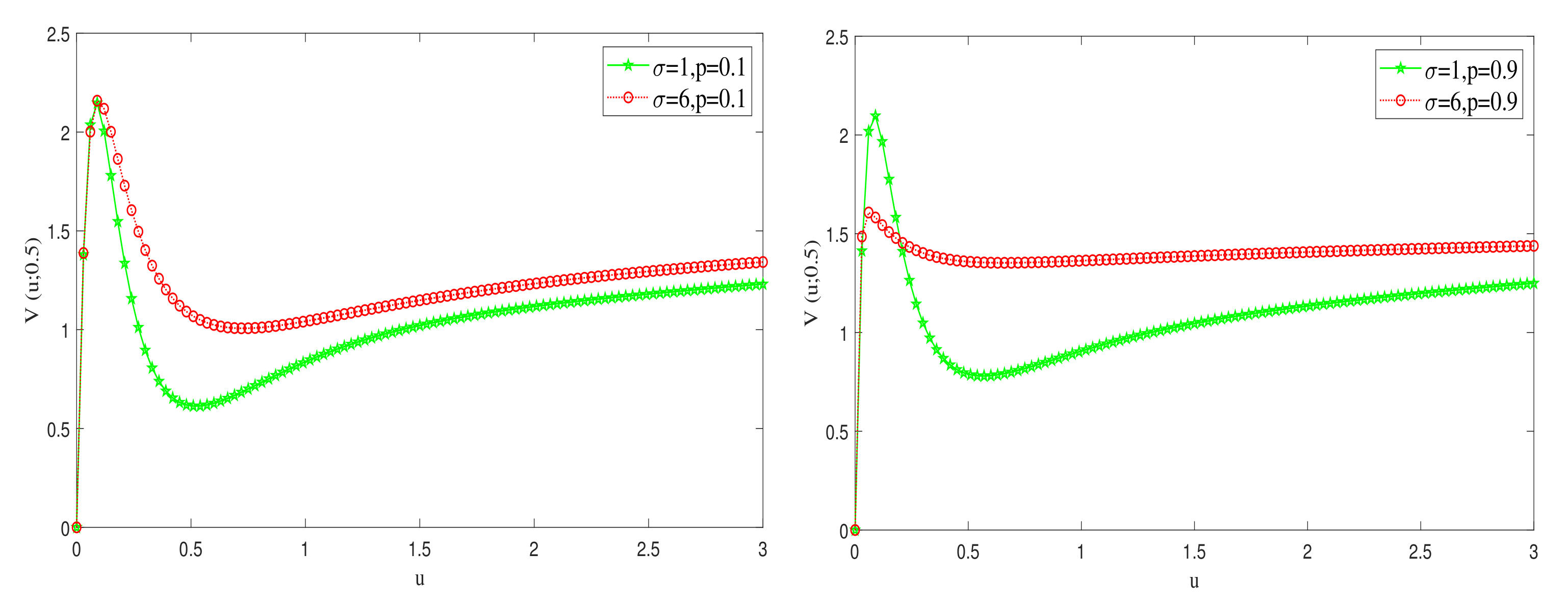
From Figure 2, we can see the impact of the parameter σ on the results of $V(u;0.5)$ for $u\in [0,3]$ under $\sigma =1$ and $\sigma =6$. It can be seen that the change of parameter σ has a great impact on $V(u;0.5)$, significantly when the surplus is invested in risky assets in large quantities. This is also in line with reality. Because the volatility rate of risky assets σ increases, it means that investment in risky assets may gain more profits, but it may also have more losses.

Example 3. 

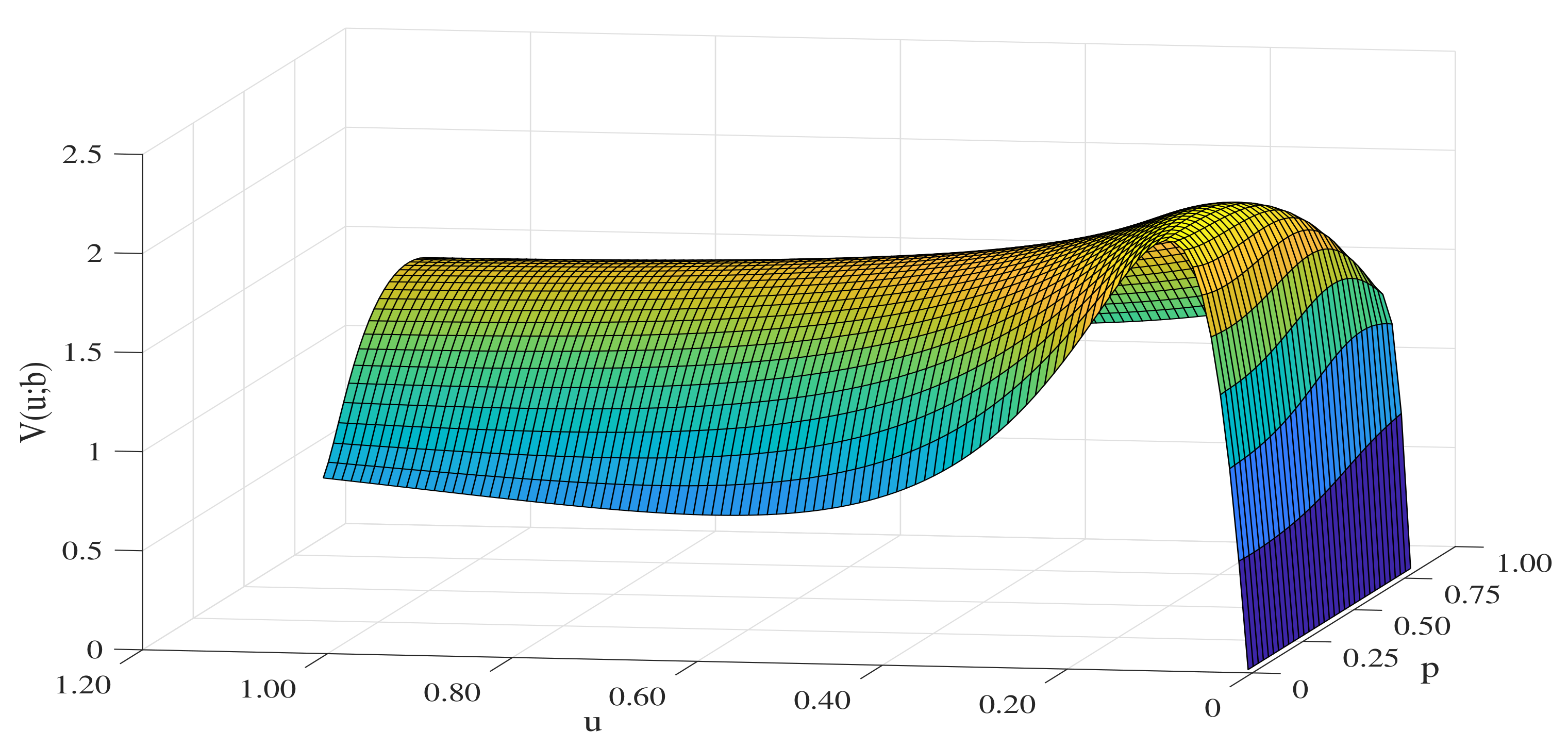
From Figure 3 and Figure 4, we can see the impact of the parameter ${\lambda }_2$ on the results of $V(u;b)$ for $u\in [0,1]$ under ${\lambda }_2=1$ and ${\lambda }_2=0$. Suppose that the optimal strategy is ${\pi }^{*}=(p_t^{{\pi }^{*}},{\alpha }_t^{{\pi }^{*}})\in \mathsf{\Pi }$, of which ${\alpha }_t^{{\pi }^{*}}=\alpha =0.1$, and find the optimal investment proportion $p_t^{{\pi }^{*}}$ within $u\in [0,1]$. The image obtained by data fitting (we give some data, see

Table 3. The values of $V(u;0.5)$ when ${\lambda }_2=1,\mu =1,\delta =0.06,c=0.4,\alpha =0.1$.

u	$\mathit{p}=0.06$	$\mathit{p}=0.21$	$\mathit{p}=0.36$	$\mathit{p}=0.51$	$\mathit{p}=0.54$	$\mathit{p}=0.69$	$\mathit{p}=0.84$	$\mathit{p}=0.99$
$0.15$	1.9361	2.0904	2.1049	2.0473	2.0275	1.8774	1.6303	1.3118
$0.35$	1.0918	1.6053	1.7960	1.8300	1.8225	1.7152	1.4964	1.2038
$0.55$	0.8657	1.4111	1.6660	1.7408	1.7391	1.6550	1.4576	1.1877
$0.75$	0.8621	1.3516	1.6177	1.7042	1.7045	1.6314	1.4493	1.1968
$0.95$	0.9173	1.3420	1.6015	1.6899	1.6908	1.6234	1.4516	1.2115

and

Table 4. The values of $V(u;0.5)$ when ${\lambda }_2=0,\mu =1,\delta =0.06,c=0.4,\alpha =0.1$.

u	$\mathit{p}=0.06$	$\mathit{p}=0.21$	$\mathit{p}=0.36$	$\mathit{p}=0.51$	$\mathit{p}=0.54$	$\mathit{p}=0.69$	$\mathit{p}=0.84$	$\mathit{p}=0.99$
$0.15$	1.1381	1.4167	1.5262	1.5219	1.5088	1.3768	1.1310	0.9422
$0.35$	0.7524	1.2371	1.4502	1.5001	1.4940	1.3859	1.1565	0.9781
$0.55$	0.6953	1.1879	1.4371	1.5102	1.5073	1.4114	1.1948	1.0256
$0.75$	0.7558	1.2043	1.4562	1.5330	1.5306	1.4387	1.2313	1.0693
$0.95$	0.8407	1.2395	1.4829	1.5572	1.5546	1.4641	1.2631	1.1065

). When there is the upward jumps, $V(u;b)$ will be higher, and when the initial surplus of the insurance company is large enough, the optimal investment proportion will be larger (i.e., more of the surplus will be invested in the risky assets).

As can be seen from the above examples, the upward jumps have a big impact on dividend payments. When the parameter ${\lambda }_2$ of the upward jumps are large, the dividend payments are also large. Insurance companies with large initial surplus are more inclined to invest most of their surplus in risky assets to gain more profits. In contrast, insurance companies with small initial surpluses will invest most of their surplus in risk-free assets. In addition, we can see that the volatility rate of risky assets $\sigma$ increases, it means that investment in risky assets may gain more profits, but it may also have more losses. This is also realistic. Finally, we obtain an optimal strategy through data fitting to maximize the dividend payments.

7. Conclusions

In this paper, we consider the proportional investment in the two-sided jumps model. In existing literature, most of the models considered are classical or dual risk models. We found that the two-sided jumps risk model is also of great practical significance through consulting the literature (see [12,13,14,15,16,30,45,46,47,48]). However, due to the complexity and processing difficulty of the two-sided jumps risk model, few scholars consider investing the surplus of the insurance companies. To solve this problem, we found a good method: sinc numerical method; however, there are some limitations to this approach. For example, in the analysis error, we give an upper limit for the error between the SA and the ES. Because the ES of the equation is difficult to obtain, we can only give the exact result of the error in special cases. Perhaps with the further research in the future, we may find a way to solve the ES of this model. In addition to the limitations of the method itself, on the application side, detailed premium income and claim data of insurance companies involve trade secrets and are difficult to obtain. Therefore, we cannot conduct further research and analysis under the econometric model. On this point, we will try to cooperate with insurance companies in the future.

In addition, our model can be extended as follows: (i) We can consider the Gerber–Shiu function and the ruin probability problems. (ii) On the basis of this risk model, we can consider maximizing the expected utility of terminal wealth. (iii) Since it is impossible for insurance companies to observe earnings at any time, we can consider the model under random observation to better conform to the actual situation. (iv) We will cooperate with insurance companies to establish an econometric model based on real premium income, claims and investment data to study relevant optimal strategy issues. However, these new directions and goals may lead to new technical difficulties. We also leave these challenges for future research.

References

1. Terziolu, M.K. Advances in Econometrics, Operational Research, Data Science and Actuarial Studies: Techniques and Theories; Springer: New York, NY, USA, 2021. [Google Scholar]
2. Wüthrich, M.V.; Merz, M. Statistical Foundations of Actuarial Learning and its Applications; Springer: New York, NY, USA, 2023. [Google Scholar]
3. Wüthrich, M.V.; Merz, M. Financial Modeling, Actuarial Valuation and Solvency in Insurance; Springer: New York, NY, USA, 2013. [Google Scholar]
4. Gerber, H.U.; Shiu, E.S. On the time value of ruin. North Am. Actuar. J. 1998, 2, 48–72. [Google Scholar] [CrossRef]
5. Albrecher, H.; Cheung, E.C.; Thonhauser, S. Randomized observation periods for the compound Poisson risk model: The discounted penalty function. Scand. Actuar. J. 2013, 2013, 424–452. [Google Scholar] [CrossRef]
6. Cheung, E.C.; Liu, H. Joint moments of discounted claims and discounted perturbation until ruin in the compound Poisson risk model with diffusion. Probab. Eng. Inf. Sci. 2022, 1–31. [Google Scholar] [CrossRef]
7. Zhu, J.; Li, S. Time-consistent investment and reinsurance strategies for mean-variance insurers under stochastic interest rate and stochastic volatility. Mathematics 2020, 8, 2183. [Google Scholar] [CrossRef]
8. Pirozzi, E. On a fractional stochastic risk model with a random initial surplus and a multi-layer strategy. Mathematics 2022, 10, 570. [Google Scholar] [CrossRef]
9. Ng, A.C. On a dual model with a dividend threshold. Insur. Math. Econ. 2009, 44, 315–324. [Google Scholar] [CrossRef]
10. Bayraktar, E.; Egami, M. Optimizing venture capital investments in a jump diffusion model. Math. Methods Oper. Res. 2008, 67, 21–42. [Google Scholar] [CrossRef] [Green Version]
11. Boucherie, R.J.; Boxma, O.J.; Sigman, K. A note on negative customers, GI/G/1 workload, and risk processes. Probab. Eng. Informational Sci. 1997, 11, 305–311. [Google Scholar] [CrossRef] [Green Version]
12. Cheung, E.C.; Liu, H.; Willmot, G.E. Joint moments of the total discounted gains and losses in the renewal risk model with two-sided jumps. Appl. Math. Comput. 2018, 331, 358–377. [Google Scholar] [CrossRef]
13. Martín-González, E.M.; Murillo-Salas, A.; Pantí, H. Gerber-Shiu function for a class of Markov-modulated Lévy risk processes with two-sided jumps. Methodol. Comput. Appl. Probab. 2022, 24, 2779–2800. [Google Scholar] [CrossRef]
14. Rebello, J.J.; Thampi, K. Some ruin theory components of two sided jump problems under renewal risk process. Int. Math. Forum 2017, 12, 311–325. [Google Scholar] [CrossRef]
15. Ivanovs, J. On scale functions for Lévy processes with negative phase-type jumps. Queueing Syst. 2021, 98, 3–19. [Google Scholar] [CrossRef]
16. Zhang, L. The Erlang (n) risk model with two-sided jumps and a constant dividend barrier. Commun. Stat. Theory Methods 2021, 50, 5899–5917. [Google Scholar] [CrossRef]
17. Zhuo, W.; Yang, H.; Chen, X. Expected discounted penalty function for a phase-type risk model with stochastic return on investment and random observation periods. Kybernetes 2018, 47, 1420–1434. [Google Scholar] [CrossRef]
18. Oseni, B.M.; Jolayemi, E.T. Ruin probabilities in perturbed risk process with stochastic investment and force of interest. Kybernetes 2018, 13, 1593–1608. [Google Scholar] [CrossRef]
19. Elghribi, M. Stochastic calculus in a risk model with stochastic return on investments. Stochastics Int. J. Probab. Stoch. Processes 2020, 93, 110–129. [Google Scholar] [CrossRef]
20. Chen, S.; Li, Z.; Li, K. Optimal investment–reinsurance policy for an insurance company with VaR constraint. Insur. Math. Econ. 2010, 47, 144–153. [Google Scholar] [CrossRef]
21. Zhang, Q.; Chen, P. Robust optimal proportional reinsurance and investment strategy for an insurer with defaultable risks and jumps. J. Comput. Appl. Math. 2019, 356, 46–66. [Google Scholar] [CrossRef]
22. De Finetti, B. Su un’impostazione alternativa della teoria collettiva del rischio. In Transactions of the XVth International Congress of Actuaries; Actuarial Society of America: New York, NY, USA, 1957; Volume 2, pp. 433–443. [Google Scholar]
23. Vierkötter, M.; Schmidli, H. On optimal dividends with exponential and linear penalty payments. Insur. Math. Econ. 2017, 72, 265–270. [Google Scholar] [CrossRef]
24. Albrecher, H.; Azcue, P.; Muler, N. Optimal dividend strategies for two collaborating insurance companies. Adv. Appl. Probab. 2017, 49, 515–548. [Google Scholar] [CrossRef] [Green Version]
25. Chen, X.; Ou, H. A compound Poisson risk model with proportional investment. J. Comput. Appl. Math. 2013, 242, 248–260. [Google Scholar] [CrossRef]
26. Albrecher, H.; Azcue, P.; Muler, N. Optimal ratcheting of dividends in insurance. SIAM J. Control Optim. 2020, 58, 1822–1845. [Google Scholar] [CrossRef]
27. Dong, H.; Yin, C.; Dai, H. Spectrally negative Lévy risk model under Erlangized barrier strategy. J. Comput. Appl. Math. 2019, 351, 101–116. [Google Scholar] [CrossRef]
28. Chen, Y.; Bian, B. Optimal investment and dividend policy in an insurance company: A varied bound for dividend rates. Discret. Contin. Dyn. Syst. 2019, 24, 5083–5105. [Google Scholar] [CrossRef]
29. Bo, L.; Song, R.; Tang, D.; Wang, Y.; Yang, X. Lévy risk model with two-sided jumps and a barrier dividend strategy. Insur. Math. Econ. 2012, 50, 280–291. [Google Scholar] [CrossRef]
30. Palmowski, Z.; Vatamidou, E. Phase-type approximations perturbed by a heavy-tailed component for the Gerber-Shiu function of risk processes with two-sided jumps. Stoch. Model. 2020, 36, 337–363. [Google Scholar] [CrossRef]
31. Chen, X.; Xiao, T.; Yang, X.q. A Markov-modulated jump-diffusion risk model with randomized observation periods and threshold dividend strategy. Insur. Math. Econ. 2014, 54, 76–83. [Google Scholar] [CrossRef]
32. Gerber, H.U.; Shiu, E.S. On optimal dividend strategies in the compound Poisson model. North Am. Actuar. J. 2006, 10, 76–93. [Google Scholar] [CrossRef]
33. Schmidli, H. On minimizing the ruin probability by investment and reinsurance. Ann. Appl. Probab. 2002, 12, 890–907. [Google Scholar] [CrossRef]
34. Jgaard, B.H.; Taksar, M. Controlling risk exposure and dividends payout schemes: Insurance company example. Math. Financ. 1999, 9, 153–182. [Google Scholar] [CrossRef]
35. Albrecher, H.; Thonhauser, S. Optimal dividend strategies for a risk process under force of interest. Insur. Math. Econ. 2008, 43, 134–149. [Google Scholar] [CrossRef] [Green Version]
36. Wan, N. Dividend payments with a threshold strategy in the compound Poisson risk model perturbed by diffusion. Insur. Math. Econ. 2007, 40, 509–523. [Google Scholar] [CrossRef]
37. Wu, Y.; Wu, X. Linearized and rational approximation method for solving non-linear Burgers’ equation. Int. J. Numer. Methods Fluids 2004, 45, 509–525. [Google Scholar] [CrossRef]
38. Stenger, F. Numerical Methods Based on Sinc and Analytic Functions; Springer: New York, NY, USA, 1993. [Google Scholar]
39. Stenger, F. Handbook of Sinc Numerical Methods; CRC Press: Boca Raton, FL, USA, 2011. [Google Scholar]
40. Liu, Y.; Chen, X.; Zhuo, W. Dividends under threshold dividend strategy with randomized observation periods and capital-exchange agreement. J. Comput. Appl. Math. 2020, 366, 112426. [Google Scholar] [CrossRef]
41. Wang, C.; Deng, N.; Shen, S. Numerical method for a perturbed risk model with proportional investment. Mathematics 2023, 11, 43. [Google Scholar] [CrossRef]
42. Lund, J.; Bowers, K.L. Sinc Methods for Quadrature and Differential Equations; SIAM: Philadelphia, PA, USA, 1992. [Google Scholar]
43. Stenger, F. Summary of Sinc numerical methods. J. Comput. Appl. Math. 2000, 13, 379–420. [Google Scholar] [CrossRef]
44. Zhi, H.; Pu, J. On a dual risk model perturbed by diffusion with dividend threshold. Chin. Ann. Math. Ser. B 2016, 37, 777–792. [Google Scholar] [CrossRef]
45. Zhang, Z.; Yang, H.; Li, S. The perturbed compound Poisson risk model with two-sided jumps. J. Comput. Appl. Math. 2010, 233, 1773–1784. [Google Scholar] [CrossRef] [Green Version]
46. Cheung, E.C. On a class of stochastic models with two-sided jumps. Queueing Syst. 2011, 69, 1–28. [Google Scholar] [CrossRef] [Green Version]
47. Labbé, C.; Sendov, H.S.; Sendova, K.P. The Gerber–Shiu function and the generalized Cramér–Lundberg model. Appl. Math. Comput. 2011, 218, 3035–3056. [Google Scholar] [CrossRef]
48. Dong, H.; Liu, Z. The ruin problem in a renewal risk model with two-sided jumps. Math. Comput. Model. 2013, 57, 800–811. [Google Scholar] [CrossRef]
Figure 1. Images of V ( u ; 0.5 ) when N = 10 , α ^ = 1 4 , β ^ = 1 2 , d ^ = π 2 , σ = 6 and p = 0.1 , p = 0.9 .
Mathematics 11 01584 g001
Figure 2. Images of V ( u ; 0.5 ) when N = 10 , α ^ = 1 4 , β ^ = 1 2 , d ^ = π 2 , λ 2 = 1 and p = 0.1 , p = 0.9 .
Mathematics 11 01584 g002
Figure 3. Images of V ( u ; 0.5 ) when N = 10 , α ^ = 1 4 , β ^ = 1 2 , d ^ = π 2 , σ = 6 and λ 2 = 1 .
Mathematics 11 01584 g003
Figure 4. Images of V ( u ; 0.5 ) when N = 10 , α ^ = 1 4 , β ^ = 1 2 , d ^ = π 2 , σ = 6 and λ 2 = 0 .
Mathematics 11 01584 g004