Abstract
Deglobalization, as opposed to the term globalization, appears in the world order due to local solutions to problems and border controls, ignoring the principles of treaties, trade wars, and the expansion of regionalism. In addition, slowbalization helps shrink the global flow of trade, information, and societal and cultural exchange dynamism. However, this scary global order, as triggered by deglobalization and slowbalization, significantly impacts the income factors of allied nations. Against this background, we aim to investigate whether deglobalization and slowbalization proxied by the influencing magnitudes of globalization dimensions (e.g., globalization de facto and de jure, internet diffusions, and trade openness) impact the income inequality of the 12 post-Soviet countries, considering the panel data during 1991–2019. To this end, we apply the quantiles via moments approach to investigate the time-varying connectedness between variables that have country and data-centric heterogeneities. Our findings depict that deglobalization is futile in affecting the post-Soviet countries’ income dynamics, as globalization negatively affects income inequality in diverse quantiles. Specifically, globalization de facto (globalized policy-implementation spectrum) and internet diffusions have a significantly negative influence on reducing income inequality from low to medium quantiles (q.25–q.75). Globalization de jure (globalized policy-decision spectrum) and trade openness are statistically insignificant in entire quantiles (q.25–q.95), implying the likely existence of slowbalization. Finally, government expenditures and governance quality are monotonically negative in reducing income inequality at all quantiles (q.25–q.95). Therefore, policy suggestions enclose galvanizing globalization potentials in curbing income inequality to keep away the distressful phases of deglobalization and slowbalization.
Keywords:
deglobalization; globalization; slowbalization; internet diffusions; trade openness; quantiles via moments MSC:
91B02; 91B15; 91B60; 91B84
1. Introduction
Globalization has been one of the most well-known economic phenomena in the 21st century due to its dominant consequences in all spheres of modern life [1]. After decades of rapid globalization through the channel of the movement of technology, labor, and capital, it is argued that this trend appears to have reversed (deglobalization) or slowed down (slowbalization), from a more critical scholarly viewpoint [2]. However, in recent years, trade rivalry between the U.S. and China, the withdrawal of the United Kingdom from the European Union, the COVID-19 pandemic, and increasing geopolitical risks have shaken the seemingly secure ground underpinning the process of globalization [3]. On the other hand, the concentration of income in a few people in both developed and developing countries has led to the reconsideration of hypotheses regarding the distributional agenda of globalization [4]. However, to what extent is this questioning valid for the post-Soviet countries that have undergone an abrupt transformation from the command to the market economic system?
The notable feature of these countries is their high dependence on natural resources, particularly oil and gas. This reliance on commodity exports has made these countries vulnerable to fluctuations in global commodity prices, contributing to economic instability and income inequality. Understanding the impact of all these developments on economic inequalities in the post-Soviet nations sheds light on possible physical and virtual integration or fragmentation scenarios of globalization and their distributional consequences. Therefore, we are motivated to examine the effects of deglobalization proxied to the influencing magnitudes of globalized dimensions (e.g., globalization de facto and de jure, internet diffusions and trade openness) on general (the Gini coefficient) and percentile measures (the top 1%, 10%, and the bottom 60%) of income inequality.
Our motivation to conduct this investigation lies in strands of propositions. First, the related literature on the globalization–inequality nexus has mainly focused on generalized globalization measures [2,3,4]. However, the impact of globalization’s reverse or slow trend on the increasing economic inequalities is better understood by considering the different dimensions of globalization. Our concern regarding the considering de facto and de jure globalization measures as well as the virtual (global diffusion of internet traffic) and physical (trade openness) aspects of globalization have been neglected by the empirical literature, which motivated us to conduct this study.
Second, in the previous literature, it has been examined whether and to what extent deglobalization or slowbalization plays a role in inequality in both developed and developing countries. Nevertheless, a limited number of studies have been conducted on the impact of deglobalization on economic inequality in transition countries, particularly in post-Soviet nations. This group of countries presents several advantages. For example, because transition countries have experienced a sudden socioeconomic transformation, the distributive impact of deglobalization on social classes can be investigated much more effectively because this group of countries shared a common economic starting point. Moreover, following the collapse of communism, a sudden change in the distribution of income and wealth provides a unique research environment because the characteristics of inequality are similar in this group of countries, which would be impossible if focusing on country groups with distinct inequality structures.
Third, as a proxy for inequality, earlier investigations such as those of Dorn et al. [5] and Gozgor and Ranjan [6] used the Gini coefficient of income to measure income inequality, but this has some limitations, especially when it comes to overlooking structural changes within the population. For instance, the dominant income group of the population can be overestimated or underestimated in the Gini coefficient [7]. Thus, the Gini coefficient can remain static, even if there is an alteration in the income shares in some groups of the population. In this regard, our study uses not only the income Gini coefficient but also people’s different levels of income occupation, including the income share of the top 1%, the income shares of the top 10%, and the income share of the bottom 60% as dependent variables. Using percentile measures of inequality is significant because a large part of the widely observed increase in overall income inequality within countries can be attributed to the top income percentiles [8]. The increasing trend of top income shares has sparked public concerns about rising inequality [9] and has triggered an academic discussion about the consequences and determinants of economic inequality at the top and bottom levels, especially after the study by Piketty [10].
Lastly, whether globalization has an effective contribution to reducing income inequality has been analyzed by many researchers. There are some studies that report the positive role of globalization in reducing income inequality [3,11,12,13,14], whereas enough studies reveal that globalization leads to increasing inequality in most rich and developing countries [15,16,17,18,19]. However, this study focuses on the post-Soviet countries because of some unique features, including having weak institutions and the same inequality structures, being primarily resource-abundant economies. Due to the complex nature of the economic transition process, the fact that these countries contain elements that balance globalization/deglobalization is a very crucial reason for them to be at the center of the analysis of the relationship between globalization/deglobalization/slowbalization and inequality.
We contribute to the existing literature in four ways. First, previous literature such as Jaumotte et al. [20], Meschi and Vivarelli [21], and Silva and Leichenko [22] highlighted the role of globalization in the case of different economies’ income inequality, utilizing developed and developing country analysis. Deviating from these studies, we consider the effects of globalization dimensions on income inequality from the perspective of post-Soviet countries, which is a novel annexure to the economic literature. Second, earlier studies such as Aladejare [23], Erdoğan et al. [24], and Gygli [25] used the social, economic, and political dimensions in investigating the influences of different economic determinants. Apart from these investigations, we adopt some unique dimensions of globalization, such as globalization de facto, de jure and the virtual (global diffusion of internet traffic) and physical (trade openness) integration; we also measure their specific effect on the income inequality parameters of the post-Soviet countries. Thus, our study has significant potential in terms of variable usage.
Third, we develop a theoretical connection between the varied angles of global flow, including globalization, deglobalization, slowbalisation, and income inequality, which is our novel value added to the globalization and growth literature. Finally, this study’s findings can shed a bright light on the policymakers of the post-Soviet countries to apprehend the effects of different dimensions of globalization on people’s income share at their varied levels. This will also help provide knowledge for these policymakers concerning the magnitude of the global phenomenon’s existing contribution to the income dynamics and thereby formulate pragmatic policies for exploiting the globalized potentials for the long-run economic growth of these economies.
The remaining sections of this study are structured as follows. Section 2 includes an overview of the literature. Section 3 covers data and methodology. Section 4 outlines our key findings and discussion regarding the effect of deglobalization on income inequality. Finally, Section 5 contains the conclusion and policy implications.
2. Theoretical Underpinnings and Empirical Literature
2.1. Globalization, Deglobalization, Slowbalization and Income Inequality
Globalization mostly refers to economic integration among countries, highlighting trade and financial flows. Any hindrance and negative consequence of global economic integration on the global and country-specific economic determinants illustrates the emergence of deglobalization. On the other hand, the ineffective role of economic and other globalization parameters brings the world economy to the trajectory of slowbalization. More specifically, the effects of deglobalization on income inequality are complex because the impact of globalization’s physical (trade) and virtual (ICT) components on each country cluster is different. The World Economic Forum [26] revealed that some countries previously experienced security and ball-out issues due to the diverse countries’ attempts to nationalize their industries. This inward-looking country-specific business policy adversely affects globalization’s physical and virtual flows, triggering the momentum of deglobalization. Despite the significant reduction in global industrial output, the production quality varies significantly between regions, based on their capacity to develop local value chains and large local digital markets. The degradation of manufacturing and the long-term impact of supply shocks undermine the ability to deliver essential services (e.g., health and food). Furthermore, the virtual fragmentation of globalization increases intellectual property and knowledge conservancy, diverges data regulations and virtual services regulations, restricts freedom of speech, and intensifies cyberwarfare and misinformation [26]. All these developments lead to talent stagnation and loss of opportunities and wages for highly skilled and low-skilled workers in both developed and developing countries. In addition, due to tightening fiscal space, social safety nets fall under more pressure in most economies; hence, government spending is more likely to increase.
On the other hand, to understand the mechanisms behind the deglobalization–inequality nexus, it is significant to focus on the possible response of income inequality to physical (trade) and virtual (ICT) fragmentation of globalization. In the International Futures Model, the deglobalization–inequality link is investigated by tracing the impact of trade on an economy’s output and labor skill distribution by each sector. The labor skill distribution and capital intensity differ from industry to industry [27]. Manufacturing’s share of total value added relative to agriculture increases with the overall development and relative returns of skilled labor. In a deglobalized world, the labor share is likely to force manufacturing increases because of trade restrictions, which tend to increase the relative size of the manufacturing sector in several non-OECD countries [28]. In this case, there would be a more significant share of the workforce engaged in manufacturing, resulting in a more significant number of highly paid workers and, thus, a reduction in poverty and income inequality in the country. The reduction of foreign direct investment and imports of manufactured goods, however, hinders technological progress in poorer countries [28]. Slower technological advances result in slower productivity growth and lower wage growth in all sectors. Therefore, the composition of employees and the influence of technology on the income level of existing companies and financial institutions determine the relationship between deglobalization and income inequality. In other words, several institutional and historical factors interact in the model to determine how inequality is affected.
Characterizing the deglobalization process generally refers to the processes in which countries shift their economic activity to their local economies in every sense. This process includes trade restrictions and technological fragmentation (dual fragmentation). However, slowbalization can include a mixed impact of physical and virtual globalization. For instance, at some point over the course of slowbalization, physical fragmentation and virtual integration may occur (and vice versa) [29]. In this case, this mixed effect refers to slower and ineffective phases of globalization. According to the future-scenarios study of the World Economic Forum [26], in the case of physical fragmentation and virtual integration, physical integration is re-energized by the resumption of trade in goods, especially strategic commodities such as food, energy, and metals. However, technology is fragmenting across borders for many reasons, including cybersecurity concerns. So, virtual fragmentation leads to more substantial state control of digital freedom of speech, the development of new firewalls, inadequate privacy regulations, and an increase in misinformation risks. There are digital services and fintech, health tech, ed-tech, biotech, artificial intelligence applications, and digital currencies, among some of these technological spheres. However, state-sponsored monopolies are frequently present, which limits innovation and competition in many cases. This virtual fragmentation process affects the labor market by changing the skilled and unskilled workers’ composition [30,31]. However, physical integration may balance this inequality/equality, though economic cooperation becomes more complex with splintered digital systems. Through the diversification of their supply chains and the integration of commodities in their trade, developing countries can attract and retain global talent through the revitalization of commodity trade. So, this global trade integration affects wages [32]. Therefore, since two different effects of different aspects of globalization may coincide, the countries’ workforce composition response to these fragmentation and integration situations determines the slowbalization and income inequality relationship.
2.2. Empirical Literature
The literature on the two aspects of globalization, physical (trade openness) and virtual (ICT progress and diffusion) integration, and the income inequality nexus concerned with this study has yet to be conclusive. Most studies have focused on trade-related income inequality by considering the neoclassical trade inequality explanation for the physical aspect of globalization. In neoclassical economics, one of the most significant hypotheses is that trade can generate welfare gains. According to this central idea, countries gain from international trade, but some income groups within the countries may lose because of this trade.
The Stolper–Samuelson Theorem [33] of the Heckscher–Ohlin model has been regarded as a neoclassical framework for investigating how trade affects income distribution. In this model, the impact of trade on income distribution depends on the interrelationship between the abundance of country factors and the intensity of industry factors. As a result of the interaction between the two, greater international trade integration reduces income disparity in developing economies and increases inequality in developed economies. Based on this theoretical underpinning, some researchers report that trade integration raises income inequality [34,35,36,37,38].
Meanwhile, Gozgor and Ranjan [6] developed a theoretical model and explored how globalization affects inequality and redistribution based on their theoretical model. According to this research, when inequality increases due to globalization, a policymaker interested in maximizing the sum of welfare for all agents increases redistribution. Focusing on 140 countries, they empirically observed that globalization leads to an increase in both inequality and redistribution. In addition, Han et al. [39] examined whether regions that were exposed to globalization experienced a greater change in wage inequality compared to regions that were not exposed to globalization by using quantile regression. Contrary to what the Heckscher–Ohlin model predicted, their findings showed that the accession to the WTO was significantly associated with an increased wage disparity. Their research indicates that China’s WTO accession increased within-region wage inequality in exposed regions, as the growth of real wages at higher quantiles was relatively faster. Moreover, by using a panel quantile analysis method, another study examined the relationship between globalization and income inequality [40]. According to the findings, for technology variables, R&D expenditures tended to increase inequality by up to 50 percent, and at middle and high levels of inequality, R&D expenditures were shown to be equalized.
However, different results have also been reported in the related literature. For instance, some studies have argued that trade globalization may negatively impact income inequality [41]. Furthermore, Jaumotte et al. [20] analyzed the effects of trade globalization and financial globalization on income disparity using a sample of 51 countries. According to their findings, the overall impact can be seen as limited due to two offsetting tendencies in response to globalization. First, unlike trade integration, which has been associated with a decreased disparity, financial integration has been associated with a rising disparity. Moreover, the findings of Dreher et al. [42] reveal that globalization has escalated inequality. This has been particularly evident regarding income inequality in countries that are members of the OECD.
On the other hand, considering more than 100 countries, Figini and Görg [43] examined the nexus of inward foreign direct investment (FDI) and wage inequality in globalization’s non-international trade element. According to their findings, FDI can have different effects based on a country’s level of development. One pattern is shown for developed countries, and the other is for non-OECD countries (developing countries). In addition, there is a nonlinear relationship between wage inequality in developing countries and foreign direct investment inward stock—wage inequality increases with FDI inward stock, with this effect progressively diminishing as FDI inward stock increases. On the other hand, according to their findings, wage inequality declines with FDI inward stock in developed countries. Furthermore, no robust evidence supports the conclusion that this effect is nonlinear.
Regarding the link between the virtual aspect (ICT progress and diffusion) of globalization and income inequality, the mechanism by which technology affects the labor market is based on the hypothesis that technological progress increases wage inequality [44,45,46,47]. According to the Skill-Biased Technical Change hypothesis, there is a connection between technological advancement causing a spurt in the demand for highly skilled workers and a rise in earnings inequality. At the same time, some studies state that this hypothesis is theoretically unsuccessful [48], and many investigations [49,50] focus on the technology–inequality nexus based on this hypothesis.
He and Liu [51] provide a framework in which skill accumulation and wage inequality can be viewed as equilibrium outcomes resulting from investments in specific technological progress. Their model that uses capital-skill complementarity and endogenous skill accumulation explains much of the observed change in the relative quantity of skilled workers by accounting for the relationship between capital and skills.
On the other hand, some studies in the literature focus on the relationship between technological advancement and economic growth. For example, using a model in which heterogeneous firms have access to open trade, Perla et al. [52] investigated the interaction between technology, trade, and economic growth. According to the study, trade opens a broader range of profit opportunities through increased exports. As a result, foreign competition increases the speed at which technology is adopted and generates a faster economic growth rate. Moreover, Niebel [53] examined the ICT–economic growth linkage by considering 59 emerging, developing, and developed countries from 1995 to 2010. The findings confirmed the positive link between ICT capital and economic growth. However, the study also revealed that emerging and developing economies are not necessarily benefiting from ICT investments to the same extent as developed economies.
Meanwhile, some studies focus on the regulatory quality because a significant role in reducing the adverse effects caused by economic shocks is played by the regulatory institutions in different countries designing and implementing long-term plans to enhance governance quality [54]. In addition to institutional quality, there are also other factors that contribute to economic growth, for example, the reduction of shadow economy activities, which are related to economic inequality [55]. According to Tan [56], institutions play an important role in explaining the differences between countries across the globe. Moreover, according to the theory of equal opportunity, welfare disparities are commonly the result of circumstances, and they are the subject of compensation in a just society because they are unfair [57]. The results of this study are significant because based on the theory of equal opportunity, it is believed that welfare disparities are often the result of circumstances and should be compensated accordingly. In addition, the establishment of strong institutions is, therefore, considered to be an important component of the economy in order to eliminate this type of ethnic injustice, which has an effect on income inequality.
Regarding the debate on the effects of recent developments in globalization, the world economy has entered a phase of deglobalization in which economic agents are increasingly altering their international economic relations and shifting their economic activity to their domestic economies because of important health, economic, and policy uncertainties [58,59,60]. However, the evidence at this point strongly favors the notion of “slowbalisation”, which states that globalization’s pace has slowed considerably compared to earlier periods, rather than that of deglobalization [61]. Despite the existence of deglobalization and slowbalization in theory, no previous researchers considered them in their studies’ models and inspected the role of these two determinants (deglobalization and slowbalization) on income inequality. Thus, our analysis can add value to the existing pieces of literature in investigating the nexus between globalization, deglobalization, slowbalization, and income inequality in the context of the post-Soviet countries.
3. Materials and Methods
3.1. Data and Methodology
This study aims to investigate the influence of globalization (globalization de facto, de jure, internet diffusions, and trade openness) on the distinct forms of income inequality, including income inequality Gini coefficient and the income share of the top 1%, 10% and 60% within the purview of government expenditure and regulatory quality in the context of the 12 post-Soviet countries with panel data collected during 1991–2019. We assumed that the positive role of globalization de facto and de jure, internet diffusions, and trade openness indicate the functionality of globalization in reducing income inequality. In addition, the negative role of these parameters implies the existence of deglobalization, whereas insignificant or minimal roles illustrate the presence of slowbalization in affecting income inequality. In this study, our dependent variables are the variety of income inequality measures, such as income inequality Gini coefficient, the income share (equal split adults) of the top 1%, the income share of the top 10%, and the income share of the top 60%.
Table 1 presents variables, definitions, and sources of the data. We use percentile inequality measures because they are significant to understand which segments of society enjoy or suffer from the globalization or deglobalization and slowbalization processes, which is impossible using the Gini coefficient as a variable. The income share of the top 1% can be stated as P99–100, and it represents the fraction of total income received by the percentile with the highest income. The income share of the top 10% can be described as P90–100. It reflects the percentage of total income received by the percentile with the highest and upper-middle income levels, which can be described as the rich (P99–100) and the upper-middle (P90–99) classes. Finally, the income share of the bottom 60% can be stated as P0–60, reflecting the six lowest deciles.

Table 1.
Data definitions and sources.
In addition, we consider four dimensions of globalization indicators: globalization de facto, globalization de jure, internet diffusions and trade openness, with government expenditure and regulatory quality as the independent variables for this study. Globalization de facto and globalization de jure are indexes with a scale from 1 to 100, where 100 represents the maximum value. Globalization de facto (globalized policy-implementation spectrum) and de jure (globalized policy-decision spectrum) consist of economic, social, and political globalization measures. In addition, regulatory quality measures the perception of the government’s ability to formulate and implement sound policies and regulations that enable and promote the development of the private sector [68]. As a proxy of government expenditure, we employed general government final consumption expenditure (% of GDP). We also considered two dimensions of globalization, physical (global trade openness) and virtual (global internet diffusion) globalization, for a separate model. As a proxy of internet diffusions, we used global growth in internet traffic data, including the value of GB used per second. We also employed global trade openness data determined by the sum of exports and imports of a country as a percentage of the GDP.
3.2. Quantiles via Moments Approach
We used the quantiles via moments method [69] to analyze the study’s dataset. This method is a good fit for our study due to having a heterogeneous characteristic among our variables of interest, i.e., globalization de facto, de jure, internet diffusion and trade openness, government expenditure, regulatory quality, income inequality Gini coefficient, and the income share of the top 1%, 10% and 60% in the context of the 12 post-Soviet countries. In this case, conventional panel approaches usually fail to analyze cross-sectional heterogeneity and disparity among the panel entities. More importantly, apart from other quantile approaches, this technique can control the locational and scaling heterogeneities in the responsiveness of the dependent variable to the independent variables in the computational procedure. Hence, we can sequentially write the following equations to measure our study’s model:
where, Y denotes the dependent variable, shows the vector of the regressors, points out slope coefficients, and Z delineates a k-vector of observed differentiated (with probability value 1) conversions of the indicators of X with component 1.
where so
where .
Let’s have, ,
When using the quantile via moment approach, it is feasible to apply techniques that are only appropriate for estimating conditional means, i.e., separating cross-sectional effects in panel data models while checking how the regressors affect the conditional distribution as a whole. Koenker and Hallock [70], Cade and Noon [71], and Bassett and Koenker [72] had this information in their surveys. Moreover, this is perhaps the most remarkable characteristic of quantile regression [73,74]. In addition, this method makes it much easier to estimate complex models [75], and it yields estimates of the regression quantiles that validate a fundamental requisite frequently omitted in empirical investigations [76,77].
3.3. Driscoll Kraay’s Standard Errors Technique
We employed the Driscoll Kraay standard errors method to assess the robustness of the study findings. Due to its ability to manage disturbance terms in various panels linked to cross-sectional (spatial) dependency, this method has become an appropriate robustness checking approach. In situations where i and j are divergent panels, cross-sectional dependence is undeniable. This issue frequently arises when a set of macroeconomic data with relatively extended time periods is used [78]. First, the heteroscedasticity, cross-sectional dependency, and autocorrelation concerns are examined using the Driscoll Kraay standard errors approach. Second, this method considers the regressors’ average values when their errors are present in the model. It then uses these data in a weighted HAC estimator to provide cross-sectionally reliable standard errors [79]. The fixed effects estimator follows two steps to be executed. All variables in the model for the first step are in a transmuted form shown below:
where and . It is stated that the within-estimator concerned with the OLS estimator of is the second stage. It computes the converted regression model in Equation (13) within the framework of the pooled OLS assessment.
4. Empirical Findings
4.1. Descriptive Statistics
We start our results and discussions section by presenting the descriptive analysis of the variables of interest (Table 2). We observe that the variables’ standard deviations under ‘within’ and ‘between’ measures reveal the regular variant of our variables over time among the sample of the 12 post-Soviet countries. We also see that the standard deviation is profound for most of our variables in the “within” and “between” options, delineating the country and country-wide disparities in our sample selected for analysis. Therefore, we can appropriately utilize the quantiles via moments technique to check the heterogeneity issue among the variables and panel units.

Table 2.
Descriptive statistics.
4.2. Globalization de Facto, de Jure and Income Inequality
Using the quantiles via moments approach, we investigate the nexus between different dimensions of globalization and income inequality with its different measures. In addition, we represent respective fitted value graphs with the 95% confidence interval (CI) to prove the investigated findings yielded from the quantiles via moments. Model 1 investigates the income inequality Gini coefficient’s response to globalization de facto and globalization de jure (Table 3 and Figure 1). Our findings depict that globalization de facto negatively affects income inequality in the post-Soviet economies that we considered. The estimated coefficients of globalization de facto (GLDF) are negative and significant from q.25 to q.75. However, GLDJ is inconsequential monotonically in the entire quantiles. Regarding the effect of regulatory quality on the income inequality Gini coefficient, the estimated coefficients of REGQ are positive and significant under low and medium quantiles (q.25–q.50). On the other hand, income inequality negatively responds to government expenditure in the low quantiles. The coefficients of GOVE are insignificant at q.75 and q.95.

Table 3.
Model 1. DV: Income Inequality Gini Coefficient (INGN).
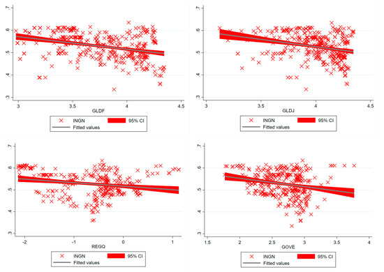
Figure 1.
Fitted values for income inequality and globalization dynamics Note: CI—Confidence interval. Legend: INGN—Income inequality Gini coefficient, GLDF—Globalization de facto; GLDJ—Globalization de jure.
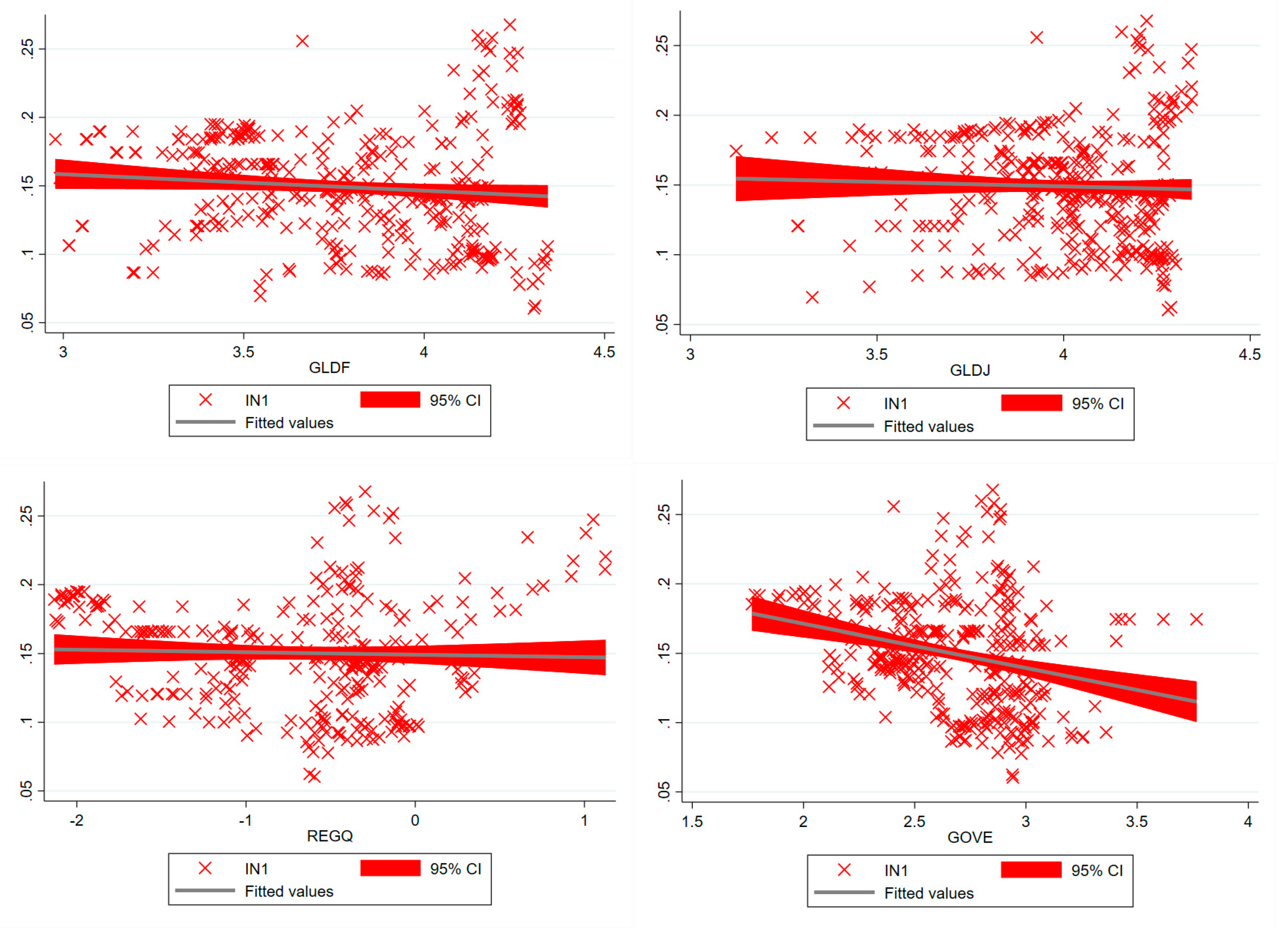
Model 2 examines the role of globalization in explaining the income share of the top 1% (Table 4 and Figure 2). The estimated coefficient of GLDF is negative and significant at q.25 and q.50. In general, GLDJ is inconsequential in entire quantiles, except from q.25. Similarly, REGQ is negligible monotonically in all the quantiles (q.25–q.95). The estimated coefficients of GOVE are negative and significant under q.25, and q.50. Focusing on the findings from top income shares is important because a large part of the widely observed increase in overall income inequality within countries is attributed to the top income percentiles [8].

Table 4.
Model 2. DV: Income Share of the Top 1% (IN1).
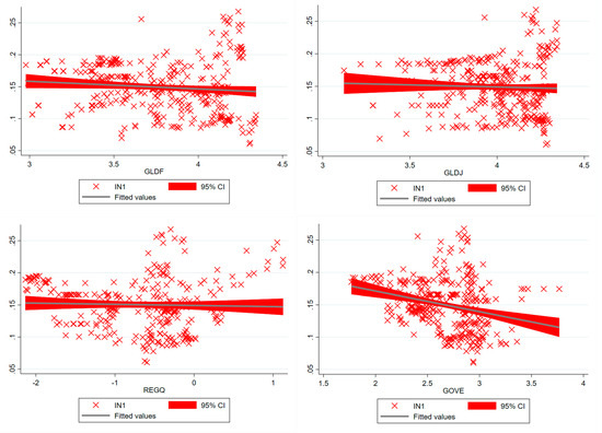
Figure 2.
Fitted values for income inequality and globalization dynamics. Note: CI—Confidence interval. Legend: IN1—The income share of the top 1%, GLDF—Globalization de facto; GLDJ—Globalization de jure.
Model 3 examines the role of globalization in the income share of the top 10% (Table 5 and Figure 3). Our findings reveal that IN2 negatively responds to GLDF. The estimated coefficients are insignificant from q.75 to q.95, as with the findings from Model 2. GLDJ has an insignificantly positive effect on IN2. Model 3 also delineates a positive and significant impact of REGQ on IN2 at q.25 and q.50. Conversely, IN2 negatively responds to GOVE at q.25 and q.50.

Table 5.
Model 3. DV: Income Share of the Top 10% (IN2).
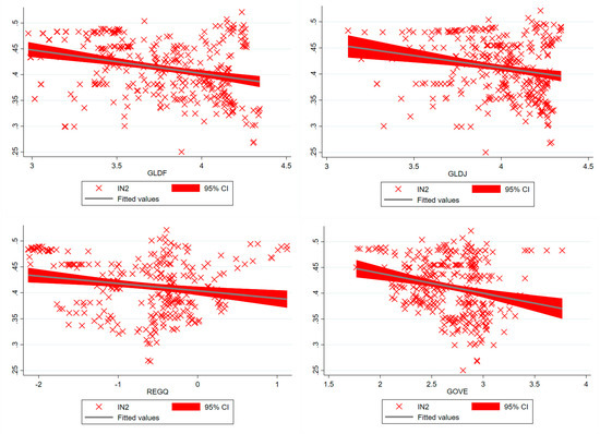
Figure 3.
Fitted values for income inequality and globalization dynamics. Note: CI—Confidence interval. Legend: IN2—The income share of the top 10%, GLDF—Globalization de facto; GLDJ—Globalization de jure.
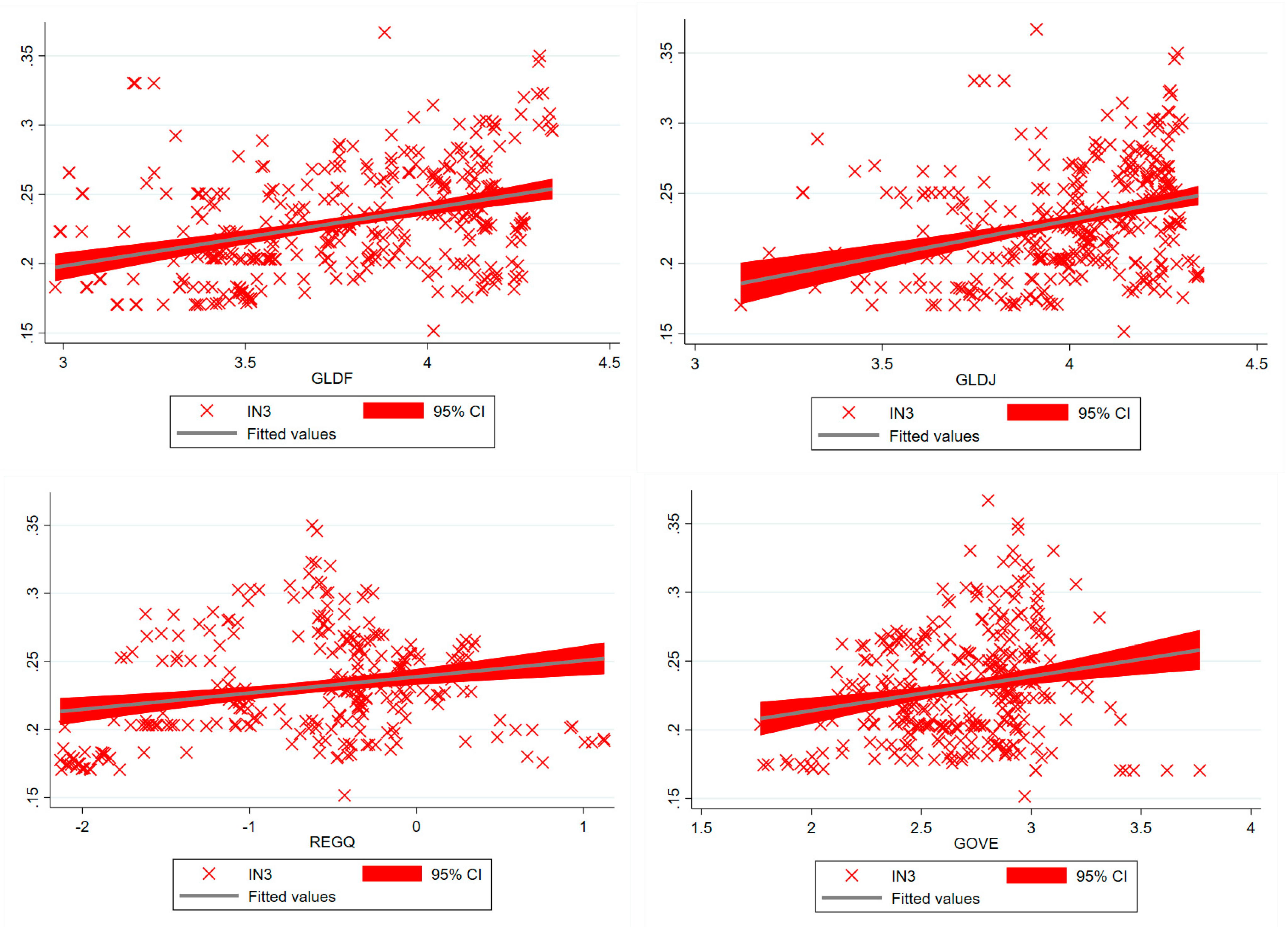
In Model 4, we investigate the response of the income share of the bottom 60% to globalization (Table 6 and Figure 4). Our findings reveal that GLDF has a positive and significant effect on IN3 from low to the extreme quantiles (q.25–q.95). The magnitude of the effect of GLDF on the bottom classes’ income increases from q.25 to q.95. Similarly, the coefficients of GLDJ are positive and significant at q.50, q75, and q.95. Regarding the role of regulatory quality, REGQ negatively influences IN3 from q.50 to q.75. The coefficient of REGQ is insignificant at q25. Our findings also show that IN3 positively responds to GOVE, with a significant coefficient from q.50 to q.95. The magnitude of globalization de facto on the top 1% income segment is higher at q.25 and q.50 than its magnitude on the bottom 60% segment of the population.

Table 6.
Model 4. DV: Income Share of the Bottom 60% (IN3).
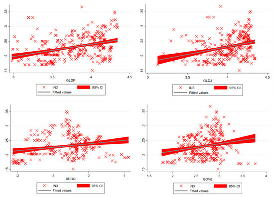
Figure 4.
Fitted values for income inequality and globalization dynamics. Note: CI—Confidence interval. Legend: IN3—The income share of the bottom 60%, GLDF—Globalization de facto; GLDJ—Globalization de jure.
4.3. Physical and Virtual Globalization and Income Inequality
In Model 5, we examine the role of physical and virtual globalization in income inequality using the quantiles via moments approach (Table 7 and Figure 5). We utilize global trade openness and global internet diffusions as a proxy for physical and virtual globalization.

Table 7.
Model 5. DV: Income Inequality Gini Coefficient (INGN).
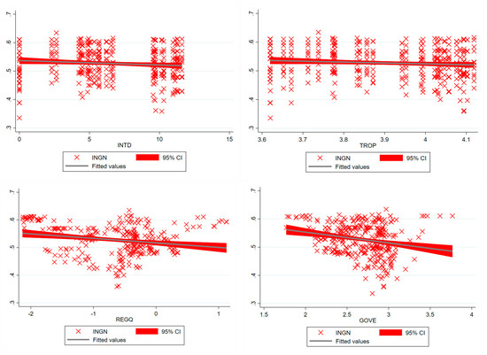
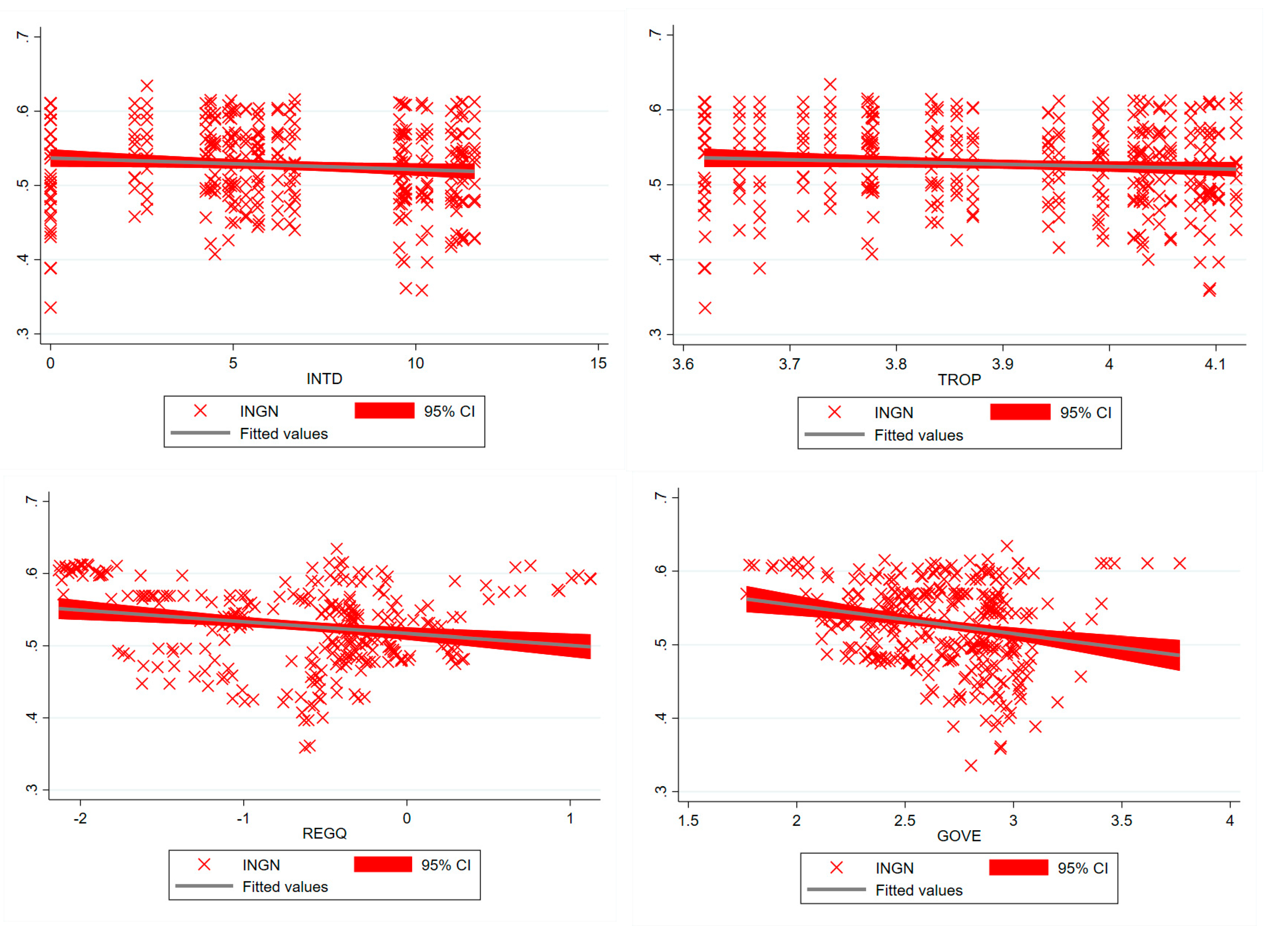
Figure 5.
Fitted values for income inequality and globalization dynamics. Note: CI—Confidence interval. Legend: INGN—Income inequality Gini coefficient, INTD—Global internet diffusions; TROP—Global trade openness.
Our findings show that global internet diffusion negatively affects the income inequality Gini coefficient in the post-Soviet economies that we considered. The estimated coefficients of global internet diffusion (INTD) are significant at q.25 and q.50. Nevertheless, global trade openness (TROP) is inconsequential monotonically in all quantiles, indicating the existence of slowbalization in explaining inequality. Regarding the effect of regulatory quality on the income inequality Gini coefficient, the estimated coefficients of REGQ are negative and significant from q.50 to q.95. On the other hand, income inequality negatively responds to government expenditure. The coefficients of GOVE are significant from q.25 and q.75.
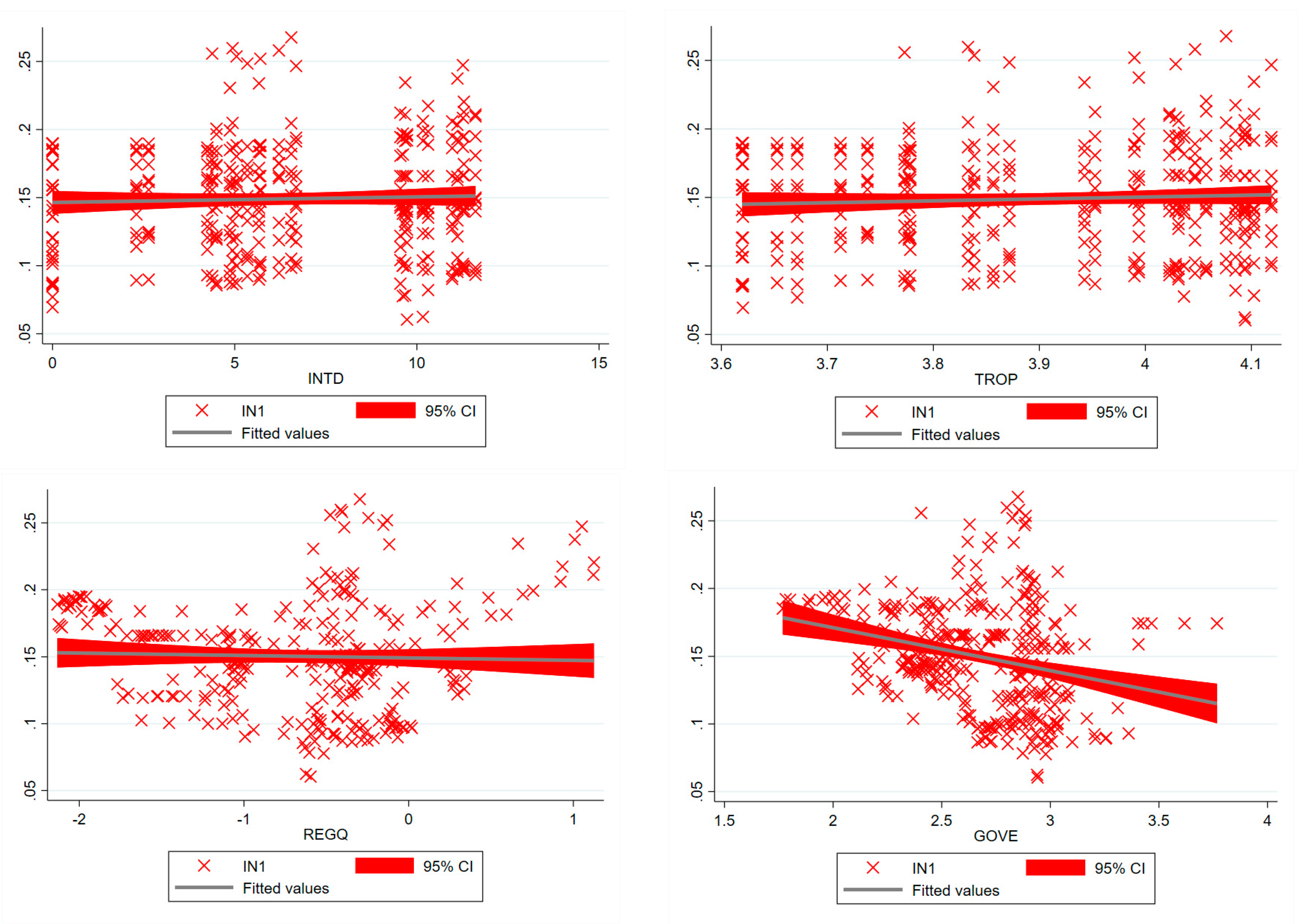
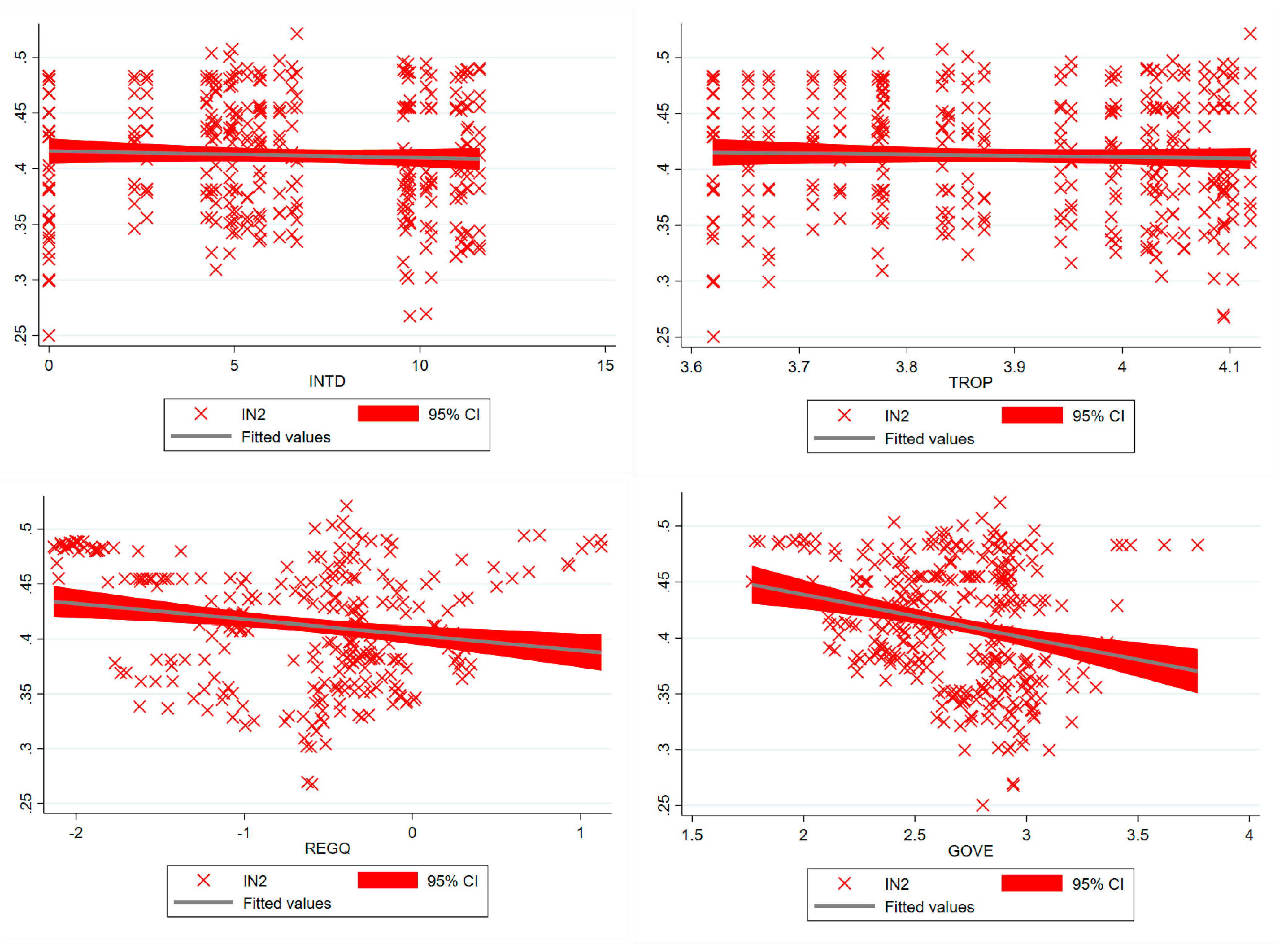
In Model 6, we investigate the response of the income share of the top 1% to physical and virtual globalization (Table 8 and Figure 6). Our findings reveal that INTD and TROP are inconsequential monotonically in entire quantiles, which indicates the existence of slowbalization in explaining the income share of the wealthy (Top 1%).

Table 8.
Model 6. DV: Income Share of the Top 1% (IN1).
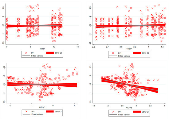
Figure 6.
Fitted values for income inequality and globalization dynamics. Note: CI—Confidence interval. Legend: IN1—The income share of the top 1%, INTD—Global internet diffusions; TROP—Global trade openness.
Model 7 examines the role of physical and virtual globalization in the income share of the top 10% (Table 9 and Figure 7). Similar to the results from Model 6, Model 7 reveals that global internet diffusion (INTD) and global trade openness (TROP) are inconsequential monotonically in entire quantiles, implying the likely existence of slowbalization. Moreover, these findings indicate that slowbalization is expected to be valid for the top income shares (P99–100 and P90–99).

Table 9.
Model 7. DV: Income Share of the Top 10% (IN2).
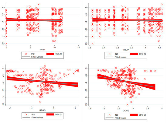
Figure 7.
Fitted values for income inequality and globalization dynamics. Note: CI—Confidence interval. Legend: IN2—The income share of the top 10%, INTD—Global internet diffusions; TROP—Global trade openness.
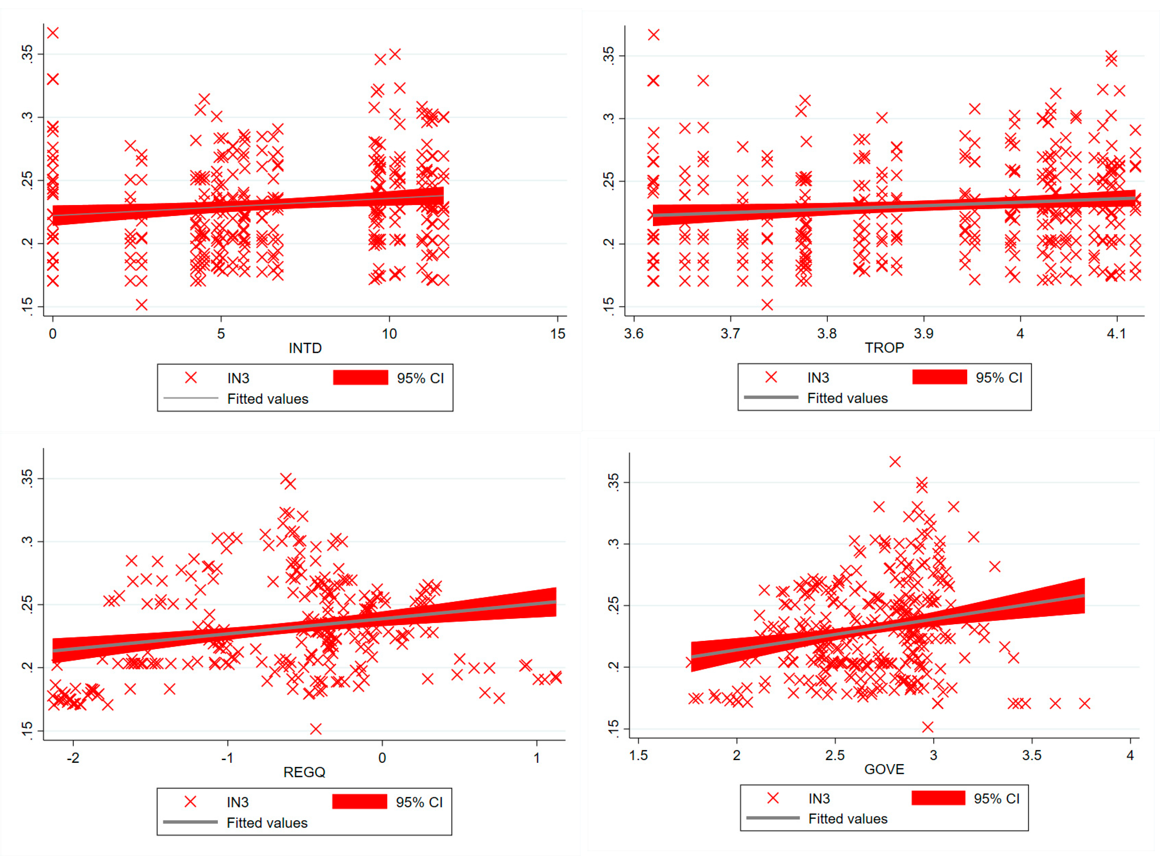
In Model 8, we investigate the response of the income share of the bottom 60% to physical and virtual globalization (Table 10 and Figure 8). Our findings reveal that INTD has a positive and significant effect on IN3 from q.25 to q.50. The results from Model 8 reveal that the estimated coefficients of TROP are positive but insignificant in all quantiles (q.25–q.95).

Table 10.
Model 8. DV: Income Share of the Bottom 60% (IN3).
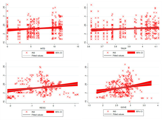
Figure 8.
Fitted values for income inequality and globalization dynamics. Note: CI—Confidence interval. Legend: IN3—The income share of the bottom 60%, INTD—Global internet diffusions; TROP—Global trade openness.
4.4. Robustness Check
4.4.1. Globalization de Facto, de Jure and Income Inequality
As a robustness check, in this part of the study, we examine the role of globalization de facto and de jure, and physical and virtual globalization in income inequality using Driscoll Kraay’s standard errors (DKSE) method. We start with investigating the impact of globalization de facto and globalization de jure on the generalized measure of income inequality, specifically the Gini coefficient (Table 11). Our findings depict that globalization de facto and globalization de jure negatively affect the income inequality Gini coefficient in post-Soviet countries. Consistent with the results we obtained in the quantiles via moments method, only the coefficient of GLDF is significant among the two components of globalization.

Table 11.
Model 1. DV: Income Inequality Gini Coefficient (INGN).
Model 2 investigates the role of globalization in explaining the income share of the top 1% by employing Driscoll Kraay’s standard errors (DKSE) method (Table 12). The estimated coefficient of GLDF is negative and significant. Our results are in line with the results from the quantiles via moments technique. Similarly, GLDJ is still inconsequential when we apply this method.

Table 12.
Model 2. Income Share of the Top 1% (IN1).
Model 3 examines the role of globalization in the income share of the top 10% (Table 13). Again, our findings reveal that IN2 negatively responds to GLDF. On the other hand, GLDJ has an insignificantly positive effect on IN2, as in the previous results.

Table 13.
Model 3. DV: Income Share of the Top 10% (IN2).
In Model 4, we investigate the response of the income share of the bottom 60% to globalization (Table 14). Our findings reveal that GLDF has a positive and significant effect on IN3, which is consistent with the results of Model 4 drawn from the quantiles via moments method (Table 6). However, the coefficients of GLDJ are positive but insignificant, contrary to the other earlier results from the quantiles via moments.

Table 14.
Model 4. DV: Income Share of the Bottom 60% (IN3).
4.4.2. Physical and Virtual Globalization and Income Inequality
In Model 5, we examine the role of physical and virtual globalization in income inequality using Driscoll Kraay’s standard errors (DKSE) method (Table 15). Our findings show that global internet diffusion negatively affects the income inequality Gini coefficient. Nevertheless, while global trade openness (TROP) is negative and inconsequential monotonically in all quantiles with the quantiles via moments approach, its effect is negative and significant with the DKSE method.

Table 15.
Model 5 DV: Income Inequality Gini Coefficient.
In Model 6, we investigate the response of the income share of the top 1% to physical and virtual globalization (Table 16). As with the findings with the quantiles via moments method, our results with the DKSE method reveal that INTD and TROP have insignificant or minimal roles in affecting top income share (the top 1%), which illustrates the presence of slowbalization.

Table 16.
Model 6. Income Share of the Top 1% (IN1).
Model 7 examines the role of physical and virtual globalization in the income share of the top 10% (Table 17). As with the findings from Model 7 with the quantiles via moments method, the results from Model 7 with the DKSE approach reveal that TROP has insignificant or minimal roles in affecting the income share of the top 10%, indicating that the existence of slowbalization is likely to be valid for top income shares (P99–100 and P90–99).

Table 17.
Model 7. DV: Income Share of the Top 10% (IN2).
In Model 8, we investigate the response of the income share of the bottom 60% to physical and virtual globalization using the DKSE method (Table 18). Our findings reveal that INTD has a positive and significant effect on IN3. In addition, the results from Model 8 indicate that the estimated coefficients of TROP are positive and significant.

Table 18.
Model 8. DV: Income Share of the Bottom 60% (IN3).
Overall, the findings have minimal differences in the estimation outcomes using the quantiles via moments and the Driscoll and Kraay standard error techniques. Despite this, we can consider the robustness of our results in explaining the relationship between globalization’s different dimensions and income inequality in the context of post-Soviet nations.
5. Discussion
Our findings depict that deglobalization is futile in affecting the post-Soviet countries’ income dynamics due to the counterproductive effect of globalization dimensions. Specifically, globalization de facto (globalized policy-implementation spectrum) is favorable in reducing income inequality in the 12 post-Soviet countries. Globalization is a multifaceted phenomenon that is achieved in various ways. International migration, information and communication technologies (ICT), trade liberalization, financial openness, and capital flows are some of its primary drivers [18,20,80,81]. One school of thought contends that globalization has reduced inequality globally by enhancing total incomes, both relative and absolute, through trade liberalization and more financial integration [82]. The other contends that while globalization increases income, the advantages do not spread equitably, increasing inequality within and between nations.
Globalization may result in more or lesser inequality in developed and developing economies, depending on the specific driving force. In the case of the 12 post-Soviet nations, financial integration played a pivotal role, which helped them entirely exploit the potential of different financial channels. Therefore, these economies absorb the fruits of globalization, reducing their income inequality through policymakers’ attempts to make a globalization-friendly business environment. In this way, foreign investors have employed their funds in the capital-intensive sectors and developed the local firms’ capacity to produce. As a result, firms’ development promotes the employment level and income level of the people. The findings concerning the positive role of globalization in reducing income inequality is in line with previous studies, including [3,11,13]. In any case, enough studies have concluded that globalization leads to increasing inequality in most rich and developing countries [15,17].
Trade liberalization induces income disparity across nations. However, trade flows help promote high-technology exports, hampering equality in the periphery. In general, trade openness correlates with every country. In this regard, Goldberg and Pavcnik [17] and Kraay [83] discovered a significant positive relationship between trade openness and inequality. However, after evaluating several studies and various indicators of trade openness (degree of trade protection, the proportion of imports or exports in GDP), they concluded that trade openness does not have an equalizing effect in emerging nations. Although this conclusion needed to be made more explicit in the four globalization routes they examined, they could not establish a causal relationship between them. They also concluded that the specific mechanisms by which globalization impacted inequality depended on the country, the time period, and the case at hand. This ineffective role of globalization indicates the existence of slowbalization, where globalization is more or less futile in stimulating income dynamics. This finding is in line with our study’s result in the case of the 12 post-Soviet countries. Similarly, Wu and Hsu’s [84] cross-sectional research pointed to an equalizing impact of global commerce on income distribution. Finally, the findings presented by Jalil [85] supported that trade openness and inequality in China have a non-linear connection. He concluded that although inequality rises with the rising trend of trade openness, inequality can decline after a crucial point.
The abovementioned discussions relating to the trade openness–income inequality nexus imply that long-term inequality reduction may occur from continued trade expansion. However, post-Soviet nations’ inaptitude for absorbing the potential of market liberation and the adaptability of domestic markets (i.e., intra-national labor and capital mobility) are the fundamental cause of the dysfunctionality of this common globalized determinant known as trade openness. Thus, slowbalization exists in these economies due to the ineffective role of globalization, as found in our study’s findings.
Internet diffusions lead to informing people’s search for their businesses. Due to the rapid evolution of information and communication technology (ICT), the body of literature highlighted the importance of the growth and effectiveness of the Internet [86,87]. However, some researchers attempted to investigate how the Internet can reduce wealth inequality [88]. An economy brings together a wide diversity of people working and living together because a country serves as the primary geographic border of human economic activities. According to one theory, countries with more internet access can utilize more resources, skilled labor, infrastructure, and resources [89]. As a result, it may be a blessing for workers and economies, as the internet diffusions help utilize relevant human and physical resources.
Another argument is that by moving specific downstream and ancillary industries to small cities, the Internet encourages technological innovation, boosts labor demand, and provides job opportunities. Small-town workers gain from manufacturing agglomeration without having to pay the congestion cost, and their marginal income from using the Internet is higher than in big cities [90,91]. In light of the potential for the rapid growth of people’s Internet access to reduce the income and wealth gap, Internet usage could be a boon for the labor force in the economy. In this case, the post-Soviet economies are still in transition in the case of exploiting the potential of the Internet. However, these economies have entered the Internet hub for reducing income inequality. Our finding is consistent with earlier studies by [92,93].
Regarding government expenditure, our finding is expected to reduce income inequality in the post-Soviet nations. This is because governments utilize fiscal policies to change the amount of expenditure to impact the overall economy. For example, the administration can use stimulus spending to boost economic activity by increasing state spending, reducing tax revenue, or combining the two [94]. Increasing government spending stimulates economic growth directly by increasing the number of goods and services purchased from the private sector or indirectly by giving people more money to spend. In order to encourage economic growth without reducing tax revenue collection, people can either increase their disposable income or spend on goods and services. More importantly, government spending aims to set all sects of entities in businesses to perform and receive the fruits of fiscal policies equally. Thus, government spending helps reduce income inequality, which is factual in the post-Soviet countries. These countries mainly assist private firms in utilizing their capital in the government-constructed infrastructure. In addition, various governments of these countries attempt to build income-generating sectors to employ the people. Therefore, these countries’ fiscal initiatives, especially government spending, help reduce income equality.
Regulatory quality depends on how the institutional mechanisms of a country function in controlling and dictating relevant organs and processes of different socio-economic and political entities. In addition, reduced income and wealth disparities contribute to less polarization in societies and are linked to the state’s institutional capabilities. The state’s institutional capacity is the ability to enact and implement laws and regulations. Many subjective indices, such as those measuring government performance, the rule of law, and corruption control, are intended to assess the competence of state institutions and whether they are powerless to bias [95]. The competency of the relevant institutions helps mobilize resources under appropriate policy implementation procedures [96]. In this case, it is unsurprising that the post-Soviet economic context reduces income inequality through mobilizing resources. These countries are primarily resource-abundant, with reserves of natural resources such as coal, natural gas, oil, and critical minerals. Moreover, resource mobilization that applies institutional mechanisms has confirmed these economies’ income inequality. This finding is in line with some studies [97,98,99,100].
6. Conclusions and Policy Implications
The focal view of this study encompasses whether globalization and its associated two reverse phenomena, deglobalization and slowbalization, are functional in affecting income inequality. Considering this view, we examined the influencing magnitude of the decomposed measures of globalization, e.g., globalization de facto and de jure, internet diffusions and trade openness on the 12 post-Soviet countries’ income inequality within the purview of government spending and regulatory quality over the period 1991–2019. Due to huge disparities among the panel units, we applied the quantiles via moments approach to investigate the time–horizon connectedness between the variables. In addition, we legitimated our findings using another robust econometric method, namely Driscoll Kraay’s standard errors (DKSE) technique. Moreover, our essential contribution to the existing literature was to test the positive and negative influence of globalization on the post-Soviet countries’ income inequality with its diverse clusters, including the income inequality Gini coefficient, the income share of the top 1%, the income share of the top 10% and the income share of the bottom 60%.
We explored some interesting findings. First, globalization de facto (globalized policy implementation spectrum) helps reduce income inequality in the case of post-Soviet economies. We observed this finding through generalized and percentile measures of inequality. Focusing on top income shares is essential, since a large portion of the population’s overall income is concentrated among the top income earners in countries with high levels of income inequality. This means that understanding the income dynamics of the top income shares can provide insight into the overall income inequality of a country. For example, the magnitude of globalization de facto in the top 1% income group is higher at q.25 and q.50 than its magnitude on the bottom 60% segment of the population. In other words, the effect of globalization on lowering the income of the rich at q.25 and q.50 is higher than its effect on increasing the income of the bottom class in the post-Soviet economies. This finding implies the implementation of the globalized policies as adopted for these economies’ progress in income and expenditure for socio-economic development. Second, internet diffusions are favorable for diminishing the income gap in these economies. However, the positive role of these two globalization parameters (globalization de facto and the Internet diffusions) indicates the non-existence of deglobalization in these countries. Third, globalization de jure (globalized policy formulation spectrum) is inconsequential in affecting income inequality. This finding is usual in the post-soviet countries’ context because of the lack of timely policy initiatives to control income inequality. Fourth, trade openness also has an ineffective role in reducing the income inequality of these countries. This finding occurs due to a lack of utilizing trade-related channels for income enhancement and income inequality reduction. Moreover, the futile influence of these two globalization dynamics (such as globalization de jure and trade openness) on income inequality illustrates the existence of slowbalization in the case of these post-Soviet economies. Fifth, government spending contributes to trimming down income inequality. This finding relates to the government’s policy measures for encouraging private business entities by providing funds and infrastructural facilities. This government scheme is critical in providing employment facilities for the people and reducing income inequality. Finally, the regulatory quality of these economies is beneficial for reducing income inequality by mobilizing resources.
We provide several policy implications. First, globalization is a multifaceted issue for diverse countries’ integration regarding socio-economic, political, informational, and cultural issues. Every country must comply with these globalized dynamics for overall development. In this regard, we observe the existence of slowbalization in the context of the post-Soviet countries due to the insignificant role of globalization de jure and trade openness. Therefore, these countries’ policymakers should formulate appropriate policies for exploiting the full-length potentials of the globalization dynamics. The partial employment or sluggish condition of this factor can push these countries onto the trajectory of deglobalization by increasing massive gaps in people’s income. Second, these countries are affluent with natural resources, which can be the catalyst for establishing a resource-based industry. This solid industry base can help connect these countries to the globalized process of trade liberation. Therefore, trade openness can substantially increase income and decrease income inequality. Notably, trade-based firms and industries can provide employment facilities to curb the disparity in income of these economies. Third, signing trade-related negotiations and treaties is a must for the industrial development of these economies, which can help reduce the income gap between the people. Fourth, these economies should attract foreign direct investment to be massively associated with globalization. This can fortify the capital base of local firms engaging all sects of people in industrial functions. Finally, we find in our study that globalization de jure, i.e., the policy adoption spectrum of these economies, is inconsequential in reducing income inequality. From this perspective, the regulatory quality of these countries should be strengthened for implementing policies relating to globalization. Authorized institutions’ stringent oversight mechanisms can prevent these economies from being engulfed by slowbalization and deglobalization. Moreover, globalization parameters can boost income and trim income inequality in post-Soviet countries.
This study only focused on certain measures of globalization, such as globalization de facto and de jure, internet diffusion, and trade openness. Future research could explore other measures of globalization to gain a better understanding of the multifaceted nature of globalization. Finally, the study only examines the impact of globalization on income inequality, but there may be other factors at play, such as education and social policies. Future research could explore the interplay between these factors and globalization to better understand the relationship between globalization and income inequality.
Author Contributions
Conceptualization, M.M.B.; Methodology, M.M.I.; Formal analysis, M.M.I.; Investigation, K.S.; Writing—original draft, M.M.B.; Writing—review & editing, M.M.I. and K.S.; Supervision, K.S. All authors have read and agreed to the published version of the manuscript.
Funding
This research received no external funding.
Data Availability Statement
Not applicable.
Conflicts of Interest
The authors declare no conflict of interest.
References
- Yeung, H.W. The Limits to Globalization Theory: A Geographic Perspective on Global Economic Change. Econ. Geogr. 2002, 78, 285–305. [Google Scholar] [CrossRef]
- Bergh, A.; Nilsson, T. Do Liberalization and Globalization Increase Income Inequality? Eur. J. Political Econ. 2010, 26, 488–505. [Google Scholar] [CrossRef]
- Asteriou, D.; Dimelis, S.; Moudatsou, A. Globalization and Income Inequality: A Panel Data Econometric Approach for the EU27 Countries. Econ. Model 2014, 36, 592–599. [Google Scholar] [CrossRef]
- Adams, S. Globalization and Income Inequality: Implications for Intellectual Property Rights. J. Policy Model 2008, 30, 725–735. [Google Scholar] [CrossRef]
- Dorn, F.; Fuest, C.; Potrafke, N. Globalisation and Income Inequality Revisited EUROPEAN. In CESifo Working Paper; Series No. 6859; European Commision: Brussels, Belgium, 2017; p. 42. [Google Scholar]
- Gozgor, G.; Ranjan, P. Globalisation, Inequality and Redistribution: Theory and Evidence. World Econ. 2017, 40, 2704–2751. [Google Scholar] [CrossRef]
- Jann, B. Assessing Inequality Using Percentile Shares. Stata J. 2016, 16, 264–300. [Google Scholar] [CrossRef]
- Leigh, A. How Closely Do Top Income Shares Track Other Measures of Inequality? Econ. J. 2007, 117, F619–F633. [Google Scholar] [CrossRef]
- Dorn, F.; Schinke, C. Top Income Shares in OECD Countries: The Role of Government Ideology and Globalisation. World Econ. 2018, 41, 2491–2527. [Google Scholar] [CrossRef]
- Piketty, T. Capital in the Twenty-First Century; Harvard University Press: Cambridge, MA, USA, 2014; ISBN 9780674369542. [Google Scholar]
- Winters, L.A.; McCulloch, N.; McKay, A. Trade Liberalization and Poverty: The Evidence so Far. J. Econ. Lit. 2004, 42, 72–115. [Google Scholar] [CrossRef]
- Kose, M.A.; Prasad, E.; Rogoff, K.; Wei, S.-J.; Rogoff, K.S. Financial Globalization: A Reappraisal. IMF Staff. Pap. 2006, 12484. [Google Scholar] [CrossRef]
- Harrison, A.; Rodríguez-Clare, A. Trade, Foreign Investment, and Industrial Policy for Developing Countries. Handb. Dev. Econ. 2010, 5, 4039–4214. [Google Scholar] [CrossRef]
- Alderson, A.; Beckfield, J.; Nielsen, F. Exactly How Has Income Inequality Changed? Patterns of Distributional Change in Core Societies. Int. J. Comp. Sociol. 2005, 46, 405–423. [Google Scholar] [CrossRef]
- Beck, T.; Demirgüç-Kunt, A.; Levine, R. Finance, Inequality and the Poor. J. Econ. Growth 2007, 12, 27–49. [Google Scholar] [CrossRef]
- Dollar, D.; Kraay, A. Trade, Growth, and Poverty. Econ. J. 2004, 114, F22–F49. [Google Scholar] [CrossRef]
- Goldberg, P.K.; Pavcnik, N. Distributional Effects of Globalization in Developing Countries. J. Econ. Lit. 2007, 45, 39–82. [Google Scholar] [CrossRef]
- Dell’Ariccia, G.; di Giovanni, J.; Faria, A.; Kose, A.; Mauro, P.; Ostry, J.D.; Schindler, M.; Terrones, M. Reaping the Benefits of Financial Globalization. IMF Occas. Pap. 2008, 264, 1–35. [Google Scholar]
- IMF. Chapter 4 Globalization and Inequality; International Monetary Fund: Washington, DC, USA, 2007; Volume 69, ISBN 9781589066885. [Google Scholar]
- Jaumotte, F.; Lall, S.; Papageorgiou, C. Rising Income Inequality: Technology, or Trade and Financial Globalization? IMF Econ. Rev. 2013, 61, 271–309. [Google Scholar] [CrossRef]
- Meschi, E.; Vivarelli, M. Trade and Income Inequality in Developing Countries. World Dev. 2009, 37, 287–302. [Google Scholar] [CrossRef]
- Silva, J.A.; Leichenko, R.M. Regional Income Inequality and International Trade. Econ. Geogr. 2004, 80, 261–286. [Google Scholar] [CrossRef]
- Aladejare, S.A. Natural Resource Rents, Globalisation and Environmental Degradation: New Insight from 5 Richest African Economies. Resour. Policy 2022, 78, 102909. [Google Scholar] [CrossRef]
- Erdoğan, S.; Çakar, N.D.; Ulucak, R.; Danish; Kassouri, Y. The Role of Natural Resources Abundance and Dependence in Achieving Environmental Sustainability: Evidence from Resource-Based Economies. Sustain. Dev. 2021, 29, 143–154. [Google Scholar] [CrossRef]
- Gygli, S.; Haelg, F.; Potrafke, N.; Sturm, J.-E.; Gygli, S.; Haelg, F.; Potrafke, N.; Sturm, J.-E. The KOF Globalisation Index—Revisited. Rev. Int. Organ. 2019, 14, 543–574. [Google Scholar] [CrossRef]
- World Economic Forum Four Futures for Economic Globalization: Scenarios and Their Implications. 2022, 8. Available online: https://www.weforum.org/whitepapers/four-futures-for-economic-globalization-scenarios-and-their-implications/ (accessed on 24 January 2023).
- Hughes, B.B.; Hossain, A.; Irfan, M. The Structure of International Futures (IFs); Routledge: Abingdon, UK, 2004. [Google Scholar]
- Hillebrand, E.E. Deglobalization Scenarios: Who Wins? Who Loses? Glob. Econ. J. 2010, 10, 1850197. [Google Scholar] [CrossRef]
- Bacchus, J. Trade Links: New Rules for a New World; Cambridge University Press: Cambridge, UK, 2022; ISBN 1009098101. [Google Scholar]
- Robinson, W.I. Transnational Processes, Development Studies and Changing Social Hierarchies in the World System: A Central American Case Study. Third World Q 2001, 22, 529–563. [Google Scholar] [CrossRef]
- Korzeniewicz, R.P.; Moran, T.P. Unveiling Inequality: A World-Historical Perspective; Russell Sage Foundation: New York, NY, USA, 2009; ISBN 1610446585. [Google Scholar]
- Gereffi, G. Global Value Chains in a Post-Washington Consensus World. Rev. Int. Polit. Econ. 2014, 21, 9–37. [Google Scholar] [CrossRef]
- Stolper, W.F.; Samuelson, P.A. Protection and Real Wages. Rev. Econ. Stud. 1941, 9, 58–73. [Google Scholar] [CrossRef]
- Chen, Z. Development and Inequality: Evidence from an Endogenous Switching Regression without Regime Separation. Econ. Lett. 2007, 96, 269–274. [Google Scholar] [CrossRef]
- Gourdon, J.; Maystre, N.; de Melo, J. Openness, Inequality and Poverty: Endowments Matter. J. Int. Trade Econ. Dev. 2008, 17, 343–378. [Google Scholar] [CrossRef]
- Helpman, E.; Itskhoki, O.; Muendler, M.-A.; Redding, S.J. Trade and Inequality: From Theory to Estimation. Rev. Econ. Stud. 2017, 84, 357–405. [Google Scholar] [CrossRef]
- Felbermayr, G.J. Dynamic Panel Data Evidence on the Trade-Income Relation. Rev. World Econ. 2005, 141, 583–611. [Google Scholar] [CrossRef]
- Rodríguez-Pose, A. Trade and Regional Inequality. Econ. Geogr. 2012, 88, 109–136. [Google Scholar] [CrossRef]
- Han, J.; Liu, R.; Zhang, J. Globalization and Wage Inequality: Evidence from Urban China. J. Int. Econ. 2012, 87, 288–297. [Google Scholar] [CrossRef]
- Han, V.; Ocal, O.; Aslan, A. A Revisit to the Relationship between Globalization and Income Inequality: Are Levels of Development Really Paramount? Qual. Quant. 2022, 57, 973–990. [Google Scholar] [CrossRef]
- Silva, J.A. Trade and Income Inequality in a Less Developed Country: The Case of Mozambique. Econ. Geogr. 2007, 83, 111–136. [Google Scholar] [CrossRef]
- Dreher, A.; Gaston, N.; Dreher, A.; Gaston, N. Has Globalization Increased Inequality? Rev. Int. Econ. 2008, 16, 516–536. [Google Scholar] [CrossRef]
- Figini, P.; Görg, H. Does Foreign Direct Investment Affect Wage Inequality? An Empirical Investigation. World Econ. 2011, 34, 1455–1475. [Google Scholar] [CrossRef]
- Bound, J.; Johnson, G.; Bound, J.; Johnson, G. Changes in the Structure of Wages in the 1980’s: An Evaluation of Alternative Explanations. Am. Econ. Rev. 1992, 82, 371–392. [Google Scholar]
- Katz, L.F.; Murphy, K.M. Changes in Relative Wages, 1963–1987: Supply and Demand Factors. Q. J. Econ. 1992, 107, 35–78. [Google Scholar] [CrossRef]
- Juhn, C.; Murphy, K.; Pierce, B.; Juhn, C.; Murphy, K.; Pierce, B. Wage Inequality and the Rise in Returns to Skill. J. Political Econ. 1993, 101, 410–442. [Google Scholar] [CrossRef]
- Acemoglu, D.; Autor, D. Skills, Tasks and Technologies: Implications for Employment and Earnings. Handb. Labor Econ. 2011, 4, 1043–1171. [Google Scholar] [CrossRef]
- Card, D.; DiNardo, J.E. Skill-Biased Technological Change and Rising Wage Inequality. J. Labor Econ. 2002, 20, 733–783. [Google Scholar] [CrossRef]
- Berman, E.; Bound, J.; Griliches, Z.; Berman, E.; Bound, J.; Griliches, Z. Changes in the Demand for Skilled Labor within U. S. Manufacturing: Evidence from the Annual Survey of Manufactures. Q. J. Econ. 1994, 109, 367–397. [Google Scholar] [CrossRef]
- Berman, E.; Bound, J.; Machin, S. Implications of Skill-Biased Technological Change: International Evidence. Q. J. Econ. 1998, 113, 1245–1279. [Google Scholar] [CrossRef]
- He, H.; Liu, Z. Investment-Specific Technological Change, Skill Accumulation, and Wage Inequality. Rev. Econ. Dyn. 2008, 11, 314–334. [Google Scholar] [CrossRef]
- Perla, J.; Tonetti, C.; Waugh, M.E. Equilibrium Technology Diffusion, Trade, and Growth. Am. Econ. Rev. 2021, 111, 73–128. [Google Scholar] [CrossRef]
- Niebel, T. ICT and Economic Growth Comparing Developing, Emerging and Developed Countries. World Dev. 2018, 104, 197–211. [Google Scholar] [CrossRef]
- Almustafa, H.; Nguyen, Q.K.; Liu, J.; Dang, V.C. The Impact of COVID-19 on Firm Risk and Performance in MENA Countries: Does National Governance Quality Matter? PLoS ONE 2023, 18, e0281148. [Google Scholar] [CrossRef] [PubMed]
- Dang, V.C.; Nguyen, Q.K.; Tran, X.H. Corruption, Institutional Quality and Shadow Economy in Asian Countries. Appl. Econ. Lett. 2022, 1–6. [Google Scholar] [CrossRef]
- Tan, C.M. No One True Path: Uncovering the Interplay between Geography, Institutions, and Fractionalization in Economic Development. J. Appl. Econom. 2010, 25, 1100–1127. [Google Scholar] [CrossRef]
- Ibragimova, Z.F.; Frants, M.V. Inequality of Opportunity: Unobserved Factors in Empirical Research. Stud. Russ. Econ. Dev. 2022, 33, 328–335. [Google Scholar] [CrossRef] [PubMed]
- Bergeijk, P. Deglobalization 2.0 Trade and Openness During the Great Depression and the Great Recession; Edward Elgar Publishing: Cheltenham, UK, 2019; ISBN 978 1 78897 345 8. [Google Scholar]
- Kataryniuk, I.; Pérez, J.; Viani, F. (De-)Globalisation of Trade and Regionalisation: A Survey of the Facts and Arguments. Occasional Papers 2124, Banco de España. 2021. Available online: https://ideas.repec.org/p/bde/opaper/2124.html (accessed on 24 January 2023).
- Lodge, D.; Everett, M.; De Bandt, O.; Georgiadis, G.; Lastauskas, P.; Carluccio, J.; Parrága, S.; Cova, P.; Attinasi, M.G.; Mozzanica, M.B.; et al. The Implications of Globalisation for the ECB Monetary Policy Strategy; Occasional Paper Series 263; European Central Bank: Frankfurt, Germany, 2021. [Google Scholar]
- Antràs, P. De-Globalisation? Global Value Chains in the Post-COVID-19 Age; Working Paper, 28115; National Bureau of Economic Research: Cambridge, MA, USA, 2020. [Google Scholar] [CrossRef]
- Data—WID—World Inequality Database. Available online: https://wid.world/data/ (accessed on 31 January 2023).
- KOF Globalisation Index—KOF Swiss Economic Institute | ETH Zurich. Available online: https://kof.ethz.ch/en/forecasts-and-indicators/indicators/kof-globalisation-index.html (accessed on 31 January 2023).
- WGI 2022 Interactive > Home. Available online: https://info.worldbank.org/governance/wgi/ (accessed on 31 January 2023).
- World Bank Open Data | Data. Available online: https://data.worldbank.org/ (accessed on 31 January 2023).
- Deglobalization | 2023 AlixPartners Disruption Index. Available online: https://disruption.alixpartners.com/alixpartners-disruption-index-2023/deglobalization/index.html (accessed on 31 January 2023).
- Feenstra, R.C.; Inklaar, R.; Timmer, M.P. The Next Generation of the Penn World Table. Am. Econ. Rev. 2015, 105, 3150–3182. [Google Scholar] [CrossRef]
- Kaufmann, D.; Kraay, A.; Mastruzzi, M. The Worldwide Governance Indicators: Methodology and Analytical Issues. Hague J. Rule Law 2011, 3, 220–246. [Google Scholar] [CrossRef]
- Machado, J.A.F.; Santos Silva, J.M.C. Quantiles via Moments. J. Econ. 2019, 213, 145–173. [Google Scholar] [CrossRef]
- Koenker, R.; Hallock, K.F. Quantile Regression. J. Econ. Perspect. 2001, 15, 143–156. [Google Scholar] [CrossRef]
- Cade, B.S.; Noon, B.R. A Gentle Introduction to Quantile Regression for Ecologists. Front Ecol Env. 2003, 1, 412–420. [Google Scholar] [CrossRef]
- Bassett, G.W.; Koenker, R.W. Strong Consistency of Regression Quantiles and Related Empirical Processes. Econ Theory 1986, 2, 191–201. [Google Scholar] [CrossRef]
- Chamberlain, G. Quantile Regression, Censoring, and the Structure of Wages. In Proceedings of the Advances in Econometrics: Sixth World Congress; Cambridge University Press: Cambridge, UK, 1994; Volume 2, pp. 171–209. [Google Scholar]
- Buchinsky, M. Changes in the US Wage Structure 1963–1987: Application of Quantile Regression. Econometrica 1994, 62, 405–458. [Google Scholar] [CrossRef]
- Nguyen, Q.K.; Yang, Z. Ownership Structure and Bank Risk-Taking in ASEAN Countries: A Quantile Regression Approach. Cogent Econ. Financ. 2020, 8, 1809789. [Google Scholar] [CrossRef]
- He, X. Quantile Curves without Crossing. Am. Stat. 1997, 51, 186–192. [Google Scholar]
- Chernozhukov, V.; Fernández-Val, I.; Galichon, A. Quantile and Probability Curves without Crossing. Econometrica 2010, 78, 1093–1125. [Google Scholar]
- Torres-Reyna, O. Panel Data Analysis Fixed and Random Effects Using Stata (v. 4.2). Data Stat. Serv. Priceton Univ. 2007, 112, 49. [Google Scholar]
- Millo, G. Maximum Likelihood Estimation of Spatially and Serially Correlated Panels with Random Effects. Comput. Stat. Data Anal. 2014, 71, 914–933. [Google Scholar] [CrossRef]
- Begg, I.; Draxler, J.; Mortensen, J. Is Social Europe Fit for Globalisation? A Study of the Social Impact of Globalisation in the European Union; The Centre for European Policy Studies (CEPS): Brussels, Belgium, 2008. [Google Scholar]
- Kose, M.A.; Prasad, E.; Rogoff, K.; Wei, S.-J.; Rogoff, K.S. Financial Globalization: A Reappraisal. IMF Staff. Pap. Palgrave Macmillan 2009, 56, 8–62. [Google Scholar] [CrossRef]
- Mills, M. Globalization and Inequality. Eur. Sociol. Rev. 2009, 25, 1–8. [Google Scholar] [CrossRef]
- Kraay, A. When Is Growth Pro-Poor? Evidence from a Panel of Countries. J. Dev. Econ. 2006, 80, 198–227. [Google Scholar] [CrossRef]
- Wu, J.Y.; Hsu, C.C. Foreign Direct Investment and Income Inequality: Does the Relationship Vary with Absorptive Capacity? Econ. Model 2012, 29, 2183–2189. [Google Scholar] [CrossRef]
- Jalil, A. Modeling Income Inequality and Openness in the Framework of Kuznets Curve: New Evidence from China. Econ. Model 2012, 29, 309–315. [Google Scholar] [CrossRef]
- Harb, G. The Economic Impact of the Internet Penetration Rate and Telecom Investments in Arab and Middle Eastern Countries. Econ. Anal. Policy 2017, 56, 148–162. [Google Scholar] [CrossRef]
- Ali, M.A.; Alam, K.; Taylor, B.; Rafiq, S. Does ICT Maturity Catalyse Economic Development? Evidence from a Panel Data Estimation Approach in OECD Countries. Econ Anal. Policy 2020, 68, 163–174. [Google Scholar] [CrossRef]
- Xun, Z.; Guanghua, W.; Jiajia, Z.; He, Z. Digital Economy, Financial Inclusion and Inclusive Growth. China Econ. 2020, 15, 92–105. [Google Scholar]
- Berger, T.; Frey, C.B. Did the Computer Revolution Shift the Fortunes of U.S. Cities? Technology Shocks and the Geography of New Jobs. Reg. Sci. Urban Econ. 2016, 57, 38–45. [Google Scholar] [CrossRef]
- Fan, J.; Tang, L.; Zhu, W.; Zou, B. The Alibaba Effect: Spatial Consumption Inequality and the Welfare Gains from e-Commerce. J. Int. Econ. 2018, 114, 203–220. [Google Scholar] [CrossRef]
- de Vos, D.; Lindgren, U.; van Ham, M.; Meijers, E. Does Broadband Internet Allow Cities to ‘Borrow Size’? Evidence from the Swedish Labour Market. Reg. Stud. 2020, 54, 1175–1186. [Google Scholar] [CrossRef]
- Liao, W.C. Inshoring: The Geographic Fragmentation of Production and Inequality. J. Urban Econ. 2012, 72, 1–16. [Google Scholar] [CrossRef]
- Fu, S.; Xu, X.; Zhang, J. Land Conversion across Cities in China. Reg. Sci. Urban Econ. 2021, 87, 103643. [Google Scholar] [CrossRef]
- Zhao, J.; Dong, K.; Dong, X.; Shahbaz, M.; Kyriakou, I. Is Green Growth Affected by Financial Risks? New Global Evidence from Asymmetric and Heterogeneous Analysis. Energy Econ. 2022, 113, 106234. [Google Scholar] [CrossRef]
- Popov, V. Developing New Measurements of State Institutional Capacity—PONARS Eurasia. 2012. Available online: https://www.ponarseurasia.org/developing-new-measurements-of-state-institutional-capacity/ (accessed on 4 January 2023).
- Islam, M.M.; Ali, M.I.; Ceh, B.; Singh, S.; Khan, M.K.; Dagar, V. Renewable and Non-Renewable Energy Consumption Driven Sustainable Development in ASEAN Countries: Do Financial Development and Institutional Quality Matter? Environ. Sci. Pollut. Res. 2022, 29, 34231–34247. [Google Scholar] [CrossRef]
- Perera, L.D.H.; Lee, G.H.Y. Have Economic Growth and Institutional Quality Contributed to Poverty and Inequality Reduction in Asia? J. Asian Econ. 2013, 27, 71–86. [Google Scholar] [CrossRef]
- Alvaredo, F.; Assouad, L.; Piketty, T. Measuring Lnequality in the Middle East 1990–2016: The World’s Most Unequal Region? Rev. Income Wealth 2019, 65, 685–711. [Google Scholar] [CrossRef]
- Asamoah, L.A. Institutional Quality and Income Inequality in Developing Countries: A Dynamic Panel Threshold Analysis. Prog. Dev. Stud. 2021, 21, 123–143. [Google Scholar] [CrossRef]
- Dolfsma, W. Government Failure: Society, Markets and Rules; Edward Elgar Publishing: Cheltenham, UK, 2013; ISBN 1782547169. [Google Scholar]
Disclaimer/Publisher’s Note: The statements, opinions and data contained in all publications are solely those of the individual author(s) and contributor(s) and not of MDPI and/or the editor(s). MDPI and/or the editor(s) disclaim responsibility for any injury to people or property resulting from any ideas, methods, instructions or products referred to in the content. |
© 2023 by the authors. Licensee MDPI, Basel, Switzerland. This article is an open access article distributed under the terms and conditions of the Creative Commons Attribution (CC BY) license (https://creativecommons.org/licenses/by/4.0/).


