Undirected Structural Markov Property for Bayesian Model Determination

Abstract

This paper generalizes the structural Markov properties for undirected decomposable graphs to arbitrary ones. This helps us to exploit the conditional independence properties of joint prior laws to analyze and compare multiple graphical structures, while being able to take advantage of the common conditional independence constraints. This work provides a theoretical support for full Bayesian posterior updating about the structure of a graph using data from a certain distribution. We further investigate the ratio of graph law so as to simplify the acceptance probability of the Metropolis–Hastings sampling algorithms.

1. Introduction

A probabilistic graphical model (PGM) or a structured probabilistic model (SPM) is a statistical model that consists of a graph and a distribution family for which the graph encodes the conditional independence information between random variables. Such models always associate with independence models, arise naturally in multivariate analysis and can provide certain versatility and convenience in analyzing complex data with large scales, while independence models are the sets of conditional independence constraints encoded by graphs via the global Markov property.

It is known that different classes of graphs with different interpretations of independence have been developed in the past decades, and the reader can refer to [1,2,3,4] for details. One of the most important classes of graphs in graphical models is undirected graphs (UGs). Their corresponding Markov models are often known as undirected graphical models or Markov networks [1,2]. These models have been found to have many applications in a wide range of areas such as econometrics, medical science, artificial intelligence [5,6,7] and so on. Our research in this paper is related to the work in the area of the structure determination of these models with the Bayesian method.

The main objective of Bayesian structure learning is to learn the structure of a graph from data. Meanwhile, Bayesian structure learning requires a clear illustration of a prior distribution about graphical structures, which is termed as a graph law. Statisticians have proposed some approaches to calculate the prior law of a graph. The simplest graph law is the uniform distribution in [8]. Additionally, the Erdös-Rényi random graph model is also used to indicate the graph law in [9]. Furthermore, a characterization of graph law with the form of exponential family is proposed by [10]. However, how to simplify this prior law is a significant task for us, especially in the posterior inference of graphical structures. In view of this, the structural Markov property is first proposed for the purpose of characterizing the conditional independence of the structure of a graph. The structural Markov properties require that the structures of distinct components of graphs are conditionally independent given the existence of a separating component; see [10]. These properties reflect the conditional independence at the structural level. It has been proved that a graph law is structural Markov if and only if it is a member of the clique exponential family given the support condition as the set of decomposable undirected graphs; see [10]. Further, a weaker support condition of equivalent characterization for graph laws is given via closure operation of graphical structures in [11].

Indeed, the structural Markov property is an extension of the hyper Markov property, which was proposed in [12] and reflects the global Markov property at the parameter level. These hyper Markov properties are used to describe the conditional independence properties of a distribution of random variables or statistical quantities in graphical models. The hyper Markov laws arise naturally as sampling distributions of maximum likelihood estimators and as prior or posterior distributions in Bayesian inference.

Recently, a weaker version of the structural Markov properties for decomposable graphs was introduced in [13], where the authors provided an analogous clique-separator factorization for the graph law. These weakly structural Markov properties require that the separator is complete. It has been shown that this provides a more flexible family of graph prior laws to use in full Bayesian posterior updating.

It should be pointed out that all the work in [8,10,13] only focuses on decomposable graphical models. However, based on conditional independence and graphical separation, the structural Markov properties might be extended to non-decomposable undirected graphical models. The aim of this paper is filling this gap in the field of graphical models. Further, we focus on a full Bayesian method for the posterior updating of graph laws via the observed data from a certain distribution, and we also prove that this full Bayesian posterior of graph law is feasible and reasonable. Finally, as examples, we illustrate our theory with detailed investigations of two significant cases based on the graphical Gaussian models and the multinomial models, respectively.

The outline of this paper is organized as follows. In Section 2, we introduce the terminologies and conceptions used in this paper. Section 3 first investigates the structural Markov properties for non-decomposable graphs, and then exploits the joint prior laws of a random sample distribution for full Bayesian inference. Section 4 gives two examples such as the inverse Wishart distribution and the Dirichlet distribution to study the posterior updating of graph laws in details. Further, we discuss some details about the computation for the structural Markov graph laws in Section 5. Finally, in Section 6, we give the conclusion of this paper.

2. Preliminaries

For terms and symbols, we follow the references [10,12] as many theoretical frameworks of this paper are constructed and developed based on them. Several concrete notions and terminologies used in this paper will be given in the following for clarity and consistency.

2.1. Graphical Terminologies and Notation

A graph $G=(V,E)$ consists of a finite set of vertices $V\left(G\right)=\{v_1,v_2,\dots ,v_p\}$ and the set of edges $E\left(G\right)\subseteq V\left(G\right)\times V\left(G\right)=\left\{\right(u,v):u,v\in V(G\left)\right\}$. An edge $(u,v)$ of G is said to be undirected if $(u,v)$ is an unordered pair. A graph G is said to be an undirected graph if all its edges are undirected. Unless otherwise specified, here G is always assumed to be undirected, simple and connected throughout the paper.

For $A\subseteq V\left(G\right)$, an induced subgraph of G on A will be denoted by $G_A=(A,E\left(G_A\right))$, where $E\left(G_A\right)=\{(u,v)\in E\left(G\right):u,v\in A\}$. All subgraphs in this paper are induced subgraphs. A is complete (or a clique) if any two different vertices $u,v\in A$ are adjacent, i.e., $(u,v)\in E\left(G\right)$. A graph is a clique if its vertex set is a clique. For $A,B\subseteq V\left(G\right)$, a clique $G_A$ is a maximal clique if $G_B$ is incomplete for any superset $B\supset A$. Two vertices u and v are considered to be neighbors if $(u,v)\in E\left(G\right)$. For $A\subseteq V\left(G\right)$, the boundary $bd\left(A\right)$ is the set of vertices in $V\left(G\right)\backslash A$ that are neighbors of vertices in A. G can be collapsible onto A if every connected component of $V\left(G\right)\backslash A$ has a complete boundary in G.

For any subsets A, B and C of $V\left(G\right)$, we say that C separates A from B, and write $A\coprod B\left|C\right[G]$, if any path in G between some $u\in A$ and $v\in B$ contains a vertex in C. Usually, we call C a separator of A and B. Separators that are cliques are called clique separators.

For any disjoint subsets A, B and S of $V\left(G\right)$, we say $(A,B,S)$ forms a decomposition if (i) $A\cup B\cup S=V\left(G\right)$; (ii) $A\coprod B\left|S\right[G]$, and (iii) S is a clique separator in G. A decomposition $(A,B,S)$ is said to be proper if the sets $A\cup S$ and $B\cup S$ are both proper subsets of $V\left(G\right)$.

Definition 1 

([14]). Let $G=(V,E)$ be an undirected graph. A graph G is reducible if its vertex set contains a clique separator, otherwise G is said to be prime. E.g., G is prime if G is a clique, while G is reducible if G is a disconnected graph. An induced subgraph $G_U$ is a maximal prime subgraph of G if it satisfies

(i) 

$G_U$ is prime, and

(ii) 

$\forall W\subseteq V\left(G\right)$ s.t. $U\subset W$, $G_W$ is reducible.

In Figure 1, it is easy to find that $G_1$ is prime since there is no clique separator in $G_1$. However, $G_2$ is reducible because of a clique separator $S=\{a,c\}$ in $G_2$.

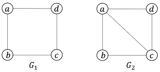
Figure 1. $G_1$ is a prime graph and $G_2$ is a reducible graph.

Definition 2 

([14]). A proper decomposition $(A,B,S)$ of an undirected graph G is stated to form a prime decomposition if $G_{A\cup S}$ and $G_{B\cup S}$ are prime, or $G_{A\cup S}$ and $G_{B\cup S}$ can be recursively decomposed into pairwise different maximal prime subgraphs of G.

In particular, G is decomposable if $G_{A\cup S}$ and $G_{B\cup S}$ are complete, or they are both decomposable subgraphs of G. Note that the prime decomposition of arbitrary undirected graphs is a generalization of that of chordal graphs. For instance, in Figure 2, G is a non-decomposable undirected graph with $V\left(G\right)=\{a,b,c,d,e\}$, which involves two maximal prime subgraphs $G_{U_1}$ and $G_{U_2}$, with $U_1=\{a,b,c\}$ and $U_2=\{b,c,d,e\}$, respectively, and a clique separator $S=U_1\cap U_2=\{b,c\}$. It is obvious that $\left(\right\{a\},\{d,e\},\{b,c\left\}\right)$ forms a prime decomposition of G. Additionally, we find that $G_{U_1}$ is complete since all its pairs of vertices are joined, while $G_{U_2}$ is incomplete because the vertices between b and d, or c and e, are not joined.

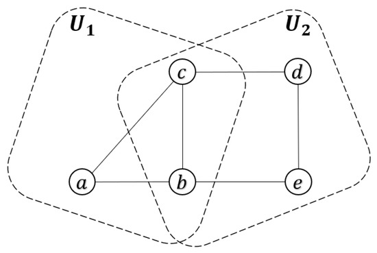
Figure 2. A prime decomposition for an undirected graph G.

It is worthwhile to point out that all the maximal prime subgraphs of an undirected graph can form a perfect sequence in a certain way. If there exists a proper decomposition of an undirected graph G, then G admits a perfect sequence $(U_1,U_2,\dots ,U_k)$ of maximal prime subgraphs, so that for each $j=2,\dots ,k$, there exists some $h\in \{1,2,\dots ,j-1\}$, and we have

$$S_j=U_j\cap (\bigcup _{i=1}^{j-1}{U}_i)\subseteq U_h,$$

where $S_j$ are clique separators actually. Specifically, G is decomposable if its all maximal prime subgraphs are complete (cliques).

In a PGM, a vertex v denotes a random variable $X_v$, which takes values in a space ${\mathfrak{X}}_v$. Let $X=X_{V\left(G\right)}={\left(X_v\right)}_{v\in V\left(G\right)}$ be a p-dimensional random vector on some product space ${\prod }_{v\in V\left(G\right)}{\mathfrak{X}}_v$ with P or $\theta$ representing its distribution. All the concerned distributions in the present paper are assumed to be positive and closed under marginalization and conditioning with respect to the type of a joint distribution family. For the sake of simplicity, we use $\mathcal{P}$ to represent the set of all positive distributions over X. For $A,B\subseteq V\left(G\right)$, ${\theta }_A$ will denote the marginal distribution of $X_A$ and ${\theta }_{B|A}$ the conditional distribution of $X_B$ given $X_A=x_A$.

Let $\mathfrak{U}$ be the set of undirected graphs with fixed vertex set $V\left(G\right)$. A probability distribution of a random graph G, which takes values in $\mathfrak{U}$, is said to be a law, denoted by $\mathfrak{G}$. Further, define $\mathfrak{U}(A,B,S)$ to be the set of undirected graphs for which $(A,B,S)$ is a prime decomposition.

2.2. Independence Model and Collapsibility

Given a finite set N, for $A,B,C\subseteq N$, an independence model, denoted by $\mathcal{I}$, is the set of triplets of the form $⟨A,B|C⟩$, which are termed as conditional independence statements. A graphical independence model is an independence model induced by a graph. For a graph $G\in \mathfrak{U}$, the graphical independence model of G can be defined as

$$\mathcal{I}\left(G\right)=\left\{⟨A,B|C⟩:A\coprod B|C\left[G\right]\mathrm{for}A,B,C\subseteq V\left(G\right)\right\}.$$

Obviously, $\mathcal{I}\left(G\right)$ is the set of triples $⟨A,B|C⟩$, encoding its global Markov property over G.

It should be pointed out that the conditional independence of a statistical model in [15,16] shares the same properties of graph separation in [2], i.e., for a graphical independence model $\mathcal{I}\left(G\right)$, it has the following properties:

• for all $A,B\subseteq V\left(G\right)$, $⟨A,B|A⟩\in \mathcal{I}(G)$, $⟨A,B|B⟩\in \mathcal{I}(G)$ and $⟨A,B|A\cap B⟩\in \mathcal{I}(G)$;
• if $⟨A,B|C⟩\in \mathcal{I}(G)$, then $⟨B,A|C⟩\in \mathcal{I}(G)$;
• if $⟨A,B|C⟩\in \mathcal{I}(G)$, and $U\subseteq A$, then $⟨U,B|C⟩\in \mathcal{I}(G)$;
• if $⟨A,B|C⟩\in \mathcal{I}(G)$, and $U\subseteq A$, then $⟨A,B|C\cup U⟩\in \mathcal{I}(G)$;
• if $⟨A,B|C⟩\in \mathcal{I}(G)$, and $⟨A,W|B\cup C⟩\in \mathcal{I}(G)$, then $⟨A,B\cup W|C⟩\in \mathcal{I}(G)$.

In particular, the following property holds when $A,B,C$ are disjoint.

If $⟨A,B|C⟩\in \mathcal{I}(G)$ and $⟨A,C|B⟩\in \mathcal{I}(G)$, then $⟨A,B\cup C|Ø⟩\in \mathcal{I}(G)$.  

Further, a graphical independence model $\mathcal{I}\left(G\right)$ has a natural projection operation on $D\subseteq V\left(G\right)$ that

$$\mathcal{I}{\left(G\right)}_D=\left\{⟨A,B|C⟩\in \mathcal{I}(G):A,B,C\subseteq D\right\}.$$

It is worthwhile to point out that $\mathcal{I}{\left(G\right)}_D\subseteq \mathcal{I}\left(G_D\right)$, where $\mathcal{I}\left(G_D\right)$ is the independence model induced by the induced subgraph $G_D$.

Definition 3 (CI-collapsibility).

Let G be a fixed undirected graph in $\mathfrak{U}$. For $D\subseteq V\left(G\right)$, $\mathcal{I}\left(G\right)$ can be conditional independence collapsible (CI-collapsible) onto D if $\mathcal{I}{\left(G\right)}_D=\mathcal{I}\left(G_D\right)$.

CI-collapsibility reflects the consistence of conditional independence relations induced by $G_D$ and those induced by G, but constrained on D.

We say a distribution P is Markov with respect to G if for $A,B,C\subseteq V\left(G\right)$, it holds that

$$⟨A,B|C⟩\in \mathcal{I}\left(G\right)\Rightarrow X_A\coprod X_B|X_C\left[P\right],$$

where $X_A\coprod X_B|X_C\left[P\right]$ represents the assertion that $X_A$ is independent of $X_B$ given $X_C$ under P.

In order to ensure that various distributions and those of statistical quantities are Markov with respect to G, we now are in a position to review the graphical models within the framework of undirected graphs. A graphical model, denoted by $\mathcal{P}\left(G\right)$, is a statistical model such that

$$\mathcal{P}\left(G\right)=\left\{P\in \mathcal{P}:X_A\coprod X_B|X_C\left[P\right]\mathrm{for}⟨A,B|C⟩\in \mathcal{I}\left(G\right)\right\}.$$

For the Markov distribution family $\mathcal{P}\left(G\right)$, we say that it is faithful to G if there exists a distribution $P^{\ast }\in \mathcal{P}\left(G\right)$ such that $\mathcal{I}\left(P^{\ast }\right)=\mathcal{I}\left(G\right)$, where

$$\mathcal{I}\left(P\right)=\left\{⟨A,B|C⟩:X_A\coprod X_B|X_C\left[P\right]\mathrm{for}A,B,C\subseteq V\left(G\right)\right\}.$$

All the graphical models concerned throughout this paper are assumed to be faithful to G. Such an assumption is called “Faithfulness Assumption” [17]. In fact, this assumption is broad and mild since Gaussian distribution families and multinomial distribution families satisfy the faithfulness assumption.

Moreover, a statistical model $\mathcal{P}\left(G\right)$ also admits a natural projection operation on $D\subseteq V\left(G\right)$, denoted by $\mathcal{P}{\left(G\right)}_D$, which is defined as follows:

$$\mathcal{P}{\left(G\right)}_D=\left\{P_D={\int }_{V\left(G\right)\backslash D}dP:P\in \mathcal{P}\left(G\right)\right\}.$$

Generally, $\mathcal{P}{\left(G\right)}_D$ is not equal to $\mathcal{P}\left(G_D\right)$, but it is obviously shown that $\mathcal{P}{\left(G\right)}_D\supseteq \mathcal{P}\left(G_D\right)$.

Definition 4 (M-collapsibility).

Let G be a fixed undirected graph in $\mathfrak{U}$. For $D\subseteq V\left(G\right)$, $\mathcal{P}\left(G\right)$ can be model collapsible (M-collapsible) onto D if $\mathcal{P}{\left(G\right)}_D=\mathcal{P}\left(G_D\right)$.

M-collapsibility indicates that the marginal distribution family is identical to the distribution family induced by $G_D$.

Theorem 1. 

Let G be a fixed undirected graph in $\mathfrak{U}$ and $D\subseteq V\left(G\right)$. Then, the following statements are equivalent.

1.

G is graphical collapsible onto D;

2.

$\mathcal{I}\left(G\right)$is CI-collapsible onto D;

3.

$\mathcal{P}\left(G\right)$is M-collapsible onto D.

Proof. 

See Appendix A.    □

Let $H_j={\bigcup }_{i=1}^j{U}_i$ denote the histories set for each $j=1,2,\dots ,k$. By Theorem 1, we can obtain the following result.

Proposition 1. 

Let G be a fixed graph in $\mathfrak{U}$ and G has a perfect sequence $(U_1,U_2,\dots ,U_k)$ of maximal prime subgraphs. Then, the following statements hold for each $j\in \{1,2,\dots ,k\}$.

1.

G can be graphical collapsible onto$H_j$;

2.

$\mathcal{I}\left(G_{H_j}\right)=\mathcal{I}{\left(G\right)}_{H_j}$;

3.

$\mathcal{P}\left(G_{H_j}\right)=\mathcal{P}{\left(G\right)}_{H_j}$.

Proof. 

This can be easily obtained from the meaning of collapsibility and Theorem 1.    □

3. Structural Markov Graph Laws for Full Bayesian Inference

3.1. Basic Concepts and Properties

We begin with the definition of the structural Markov property of [10].

Definition 5. 

A graph law $\mathfrak{G}\left(G\right)$ over $\mathfrak{U}$ is structural Markov if

$$G_{A\cup S}\coprod G_{B\cup S}|\{G\in \mathfrak{U}(A,B,S)\}\left[\mathfrak{G}\right],$$

where  $\mathfrak{G}\left(\mathfrak{U}\right(A,B,S\left)\right)>0$ and $\mathfrak{U}(A,B,S)$ is the set of undirected graphs for which $(A,B,S)$ is a prime decomposition.

Specifically, if G is decomposable in $\mathfrak{U}$, Definition 5 degenerates to that defined in [10].

The structural Markov property indicates that the structures of different induced subgraphs are conditionally independent when the event $\{G\in \mathfrak{U}(A,B,S\left)\right\}$ happens; see Figure 3 as an illustration.

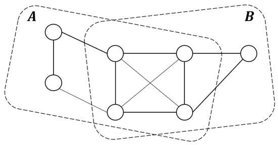
Figure 3. A representation of the structural Markov property for non-decomposable undirected graphs: $A\cap B$ is complete and separates A from B.

Proposition 2. 

Let G be a fixed undirected graph in $\mathfrak{U}$. For any subsets A, B and S of $V\left(G\right)$ satisfying $A\cup B\cup S=V\left(G\right)$, if $\mathfrak{G}\left(G\right)$ is structural Markov, then

$$G_{A\cup S}\coprod G_{B\cup S}$$

whenever S is complete and separates A from B in G.

Proof. 

By Definition 5, the existence of the remaining edges in $G_{A\cup S}$ is independent of those in $G_{B\cup S}$ since S is complete and separates A from B in G. Therefore, we are naturally left with a statement of marginal independence $G_{A\cup S}\coprod G_{B\cup S}$ since the term $G_S$ is redundant. Hence, the result follows.    □

Proposition 2 indicates that different components of undirected graphs are conditionally independent provided that their corresponding separators are complete. In order to illustrate our results with detailed investigations, we give a non-decomposable graph G in which $A\cap B$ separates A from B while $A\cap B$ is incomplete in Figure 4. We can easily find that the two subgraphs $G_B$ and $G_A$ have possible common edges in $A\cap B$, which make the existence of the remaining edges in $G_A$ dependent of those in $G_B$. In other words, these dependencies will disappear as long as $A\cap B$ is complete.

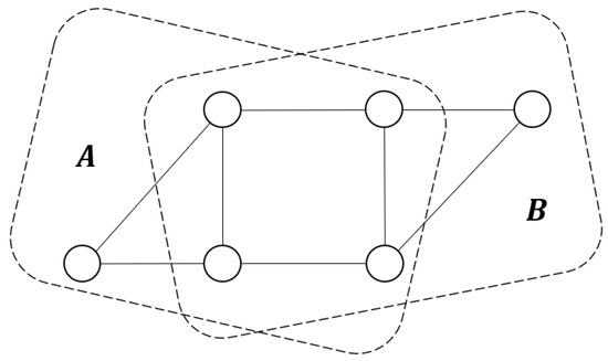
Figure 4. $A\cap B$ separates A from B while $A\cap B$ is incomplete.

It also implies that an arbitrary undirected graph can be denoted by the graph product of its induced subgraphs as

$$G=G_{A\cup S}\otimes G_{B\cup S},G\in \mathfrak{U}(A,B,S).$$

The structural Markov property can be well-characterized by the above operation.

Proposition 3. 

Let π be the density of a graph law $\mathfrak{G}$ with respect to the counting measure on $\mathfrak{U}$. Suppose that $G,G^{\prime }\in \mathfrak{U}(A,B,S)$. Then,

1.

$G_{A\cup S}\otimes G_{B\cup S}^{\prime }\in \mathfrak{U}(A,B,S)$ and $G_{A\cup S}^{\prime }\otimes G_{B\cup S}\in \mathfrak{U}(A,B,S)$;

2.

if $\mathfrak{G}$ is structural Markov on  $\mathfrak{U}$, then

$$\pi \left(G\right)\pi \left(G^{\prime }\right)=\pi (G_{A\cup S}\otimes G_{B\cup S}^{\prime })\pi (G_{A\cup S}^{\prime }\otimes G_{B\cup S}).$$

Proof. 

See Appendix A.    □

For any subset $C\subseteq A$, define $G_A^{\left(C\right)}$ to be the graph on A such that $G_A^{\left(C\right)}$ is complete in C and empty otherwise.

Proposition 4. 

Let G be a fixed graph in $\mathfrak{U}$ and G has a perfect sequence $(U_1,U_2,\dots ,U_k)$ of maximal prime subgraphs. If G has a structural Markov graph law $\mathfrak{G}$ with the density π, then the density π can be factorized as

$$\pi \left(G\right)=\frac{{\displaystyle \prod _{j=1}^k}\pi \left(G_{U_j}\right)}{{\displaystyle \prod _{j=2}^k}\pi \left(G_{S_j}\right)}.$$

(1)

Proof. 

See Appendix A.    □

3.2. Joint Distribution Law

In this section, we will investigate how the structural Markov laws interact with the hyper Markov laws when they are considered as the joint prior laws.

Hyper Markov laws are motivated by the property that graph decomposition allows one to decompose a prior or posterior distribution into the product of marginal distributions on corresponding maximal prime subgraphs. For a fixed graph $G\in \mathfrak{U}(A,B,S)$, any prior or posterior distribution of $\theta \in \mathcal{P}\left(G\right)$ is uniquely characterized by its marginals ${\theta }_{A\cup S}$ and ${\theta }_{B\cup S}$, taking values in $\mathcal{P}\left(G_{A\cup S}\right)$ and $\mathcal{P}\left(G_{B\cup S}\right)$, respectively.

Following [12], to be specific, a probability distribution of a random distribution $\theta$, which takes values in $\mathcal{P}\left(G\right)$, is said to be a law, denoted by $\mathcal{L}$. For $A\subseteq V\left(G\right)$, the marginal law of ${\theta }_A$ will be denoted by ${\mathcal{L}}_A$ and ${\mathcal{L}}_{B|A}$ will denote the conditional law of ${\theta }_{B|A}$.

Here, we give the definitions of weak and strong hyper Markov properties.

Definition 6 

([12], Weak and strong hyper Markov). Suppose that G is a fixed graph in $\mathfrak{U}(A,B,S)$ and $\theta \in \mathcal{P}\left(G\right)$. Let $\mathcal{L}\left(\theta \right)$ be a law of θ. We say that $\mathcal{L}\left(\theta \right)$ is weak hyper Markov over G if

$${\theta }_{A\cup S}\coprod {\theta }_{B\cup S}|{\theta }_S\left[\mathcal{L}\right].$$

Further, we say that$\mathcal{L}\left(\theta \right)$is strong hyper Markov over G if

$${\theta }_{A\cup S}\coprod {\theta }_{B\cup S|S}\left[\mathcal{L}\right].$$

Let X be a random sample from $\theta \in \mathcal{P}\left(G\right)$. The conditional independence property of the joint distribution law $(P,\mathcal{L})$ for the pair $(X,\theta )$ on $G\in \mathfrak{U}$ can be characterized as follows.

Proposition 5. 

Let G be a fixed undirected graph in $\mathfrak{U}$ with a prime decomposition $(A,B,S)$. X is a random sample from $\theta \in \mathcal{P}\left(G\right)$. Then, the joint distribution law of $(X,\theta )$ satisfies:

1.

if $\mathcal{L}\left(\theta \right)$ is weak hyper Markov with respect to G, then

$$(X_{A\cup S},{\theta }_{A\cup S})\coprod (X_{B\cup S},{\theta }_{B\cup S})|(X_S,{\theta }_S)[P,\mathcal{L}];$$

2.

if $\mathcal{L}\left(\theta \right)$ is strong hyper Markov, then

$$(X_{A\cup S},{\theta }_{A\cup S|S})\coprod (X_{B\cup S},{\theta }_{B\cup S})|X_S[P,\mathcal{L}].$$

Proof. 

See Appendix A.    □

It is worth mentioning that the hyper Markov property does not hold for the cases where separators are not complete. For instance, the graph $G_1$ in Figure 1 is incomplete, and we do not have ${\theta }_{\{a,b,c\}}\coprod {\theta }_{\{a,d,c\}}|{\theta }_{\{a,c\}}$ or ${\theta }_{\{b,a,d\}}\coprod {\theta }_{\{b,c,d\}}|{\theta }_{\{b,d\}}$. However, it is worthwhile to point out that the corresponding pairwise Markov property $X_b\coprod X_d|X_{\{a,c\}}$ or $X_a\coprod X_c|X_{\{b,d\}}$ holds under P if P is Markov with respect to $G_1$.

Let $\mathsf{\Theta }$ be the family of Markov distributions over $\mathfrak{U}$ and $\mathfrak{L}$ the family of hyper Markov laws over $\mathfrak{U}$. For the sake of discussion, it is necessary for us to reconsider the notion of hyper compatibility, which was first proposed by [10], to characterize families of laws for every graph.

Definition 7 (Hyper compatibility).

Let $\mathcal{L},{\mathcal{L}}^{\prime }\in \mathfrak{L}$ be the laws of $\theta \in \mathsf{\Theta }$ with respect to G and $G^{\prime }$ on $\mathfrak{U}$, respectively. For $A\subseteq V\left(G\right)$, we say $\mathfrak{L}$ is hyper compatible on $\mathfrak{U}$ if ${\mathcal{L}}_A\left(\theta \right)={\mathcal{L}}_A^{\prime }\left(\theta \right)$ whenever $G,G^{\prime }$ are collapsible onto A and $G_A=G_A^{\prime }$.

Here $\mathfrak{L}$ is always assumed to be hyper compatible over $\mathfrak{U}$. Based on the arguments above, some significant conditional independence properties of such joint law $(\mathfrak{L},\mathfrak{G})$ can be investigated as the following.

Proposition 6. 

Suppose that G has a graph law $\mathfrak{G}$ over $\mathfrak{U}$. If θ has a law $\mathcal{L}$ from a hyper compatible family $\mathfrak{L}$ over $\mathfrak{U}$, then

$${\theta }_{A\cup S}\coprod G_{B\cup S}|(G_{A\cup S},\{G\in \mathfrak{U}(A,B,S)\})[\mathfrak{L},\mathfrak{G}].$$

Proof. 

Suppose that $G\in \mathfrak{U}(A,B,S)$. Since G is collapsible onto both $A\cup S$ and $B\cup S$, by hyper compatibility, ${\mathcal{L}}_{A\cup S}$ can only take values in $\mathfrak{L}\left(G_{A\cup S}\right)$ for any $\mathcal{L}\in \mathfrak{L}$.    □

Theorem 2. 

Suppose that $\mathfrak{G}\left(G\right)$ is structural Markov over $\mathfrak{U}$. For any $\mathcal{L}\in \mathfrak{L}$,

1.

if $\mathcal{L}\left(\theta \right)$ is weak hyper Markov, then

$$({\theta }_{A\cup S},G_{A\cup S})\coprod ({\theta }_{A\cup S},G_{B\cup S})|({\theta }_S,\{G\in \mathfrak{U}(A,B,S)\})[\mathfrak{L},\mathfrak{G}];$$

2.

if $\mathcal{L}\left(\theta \right)$ is strong hyper Markov, then

$$({\theta }_{A\cup S},G_{A\cup S})\coprod ({\theta }_{B\cup S|S},G_{B\cup S})|\{G\in \mathfrak{U}(A,B,S)\}[\mathfrak{L},\mathfrak{G}].$$

Proof. 

See Appendix A.    □

Theorem 2 reflects the conditional independence properties at both parameter and structural level.

Further, for any $G\in \mathfrak{U}$, let X be a random sample from a distribution $\theta \in \mathsf{\Theta }$ on $\mathfrak{U}$. If G is assigned the prior law $\mathfrak{G}$ and $\theta$ is assigned the prior law $\mathcal{L}$, then a joint distribution law is thereby created for $(X,\theta ,G)$.

Proposition 7. 

Suppose that $\mathfrak{G}\left(G\right)$ is structural Markov on $\mathfrak{U}$. Let X be a random sample from $\theta \in \mathsf{\Theta }$. For $\mathcal{L}\in \mathfrak{L}$,

1.

if $\mathcal{L}\left(\theta \right)$ is weak hyper Markov, then

$$(X_{A\cup S},{\theta }_{A\cup S})\coprod G_{B\cup S}|(X_S,{\theta }_S,\{G\in \mathfrak{U}(A,B,S)\})[\mathsf{\Theta },\mathfrak{L},\mathfrak{G}];$$

2.

if $\mathcal{L}\left(\theta \right)$ is strong hyper Markov, then

$$(X_{A\cup S},{\theta }_{A\cup S|S})\coprod G_{B\cup S}|(X_S,\{G\in \mathfrak{U}(A,B,S)\})[\mathsf{\Theta },\mathfrak{L},\mathfrak{G}].$$

Proof. 

See Appendix A.    □

The conditional independence property of any such joint distribution law of $(X,\theta ,G)$ can be characterized as follows.

Theorem 3. 

Suppose that $\mathfrak{G}\left(G\right)$ is structural Markov on $\mathfrak{U}$. Let X be a random sample from $\theta \in \mathsf{\Theta }$ on $\mathfrak{U}$. For $\mathcal{L}\in \mathfrak{L}$,

1.

if $\mathcal{L}\left(\theta \right)$ is weak hyper Markov, then

$$(X_{A\cup S},{\theta }_{A\cup S},G_{A\cup S})\coprod (X_{B\cup S},{\theta }_{B\cup S},G_{B\cup S})|(X_S,{\theta }_S,\{G\in \mathfrak{U}(A,B,S)\})[\mathsf{\Theta },\mathfrak{L},\mathfrak{G}];$$

2.

if $\mathcal{L}\left(\theta \right)$ is strong hyper Markov, then

$$(X_{A\cup S},{\theta }_{A\cup S},G_{A\cup S})\coprod (X_{B\cup S},{\theta }_{B\cup S|S},G_{B\cup S})|(X_S,\{G\in \mathfrak{U}(A,B,S)\})[\mathsf{\Theta },\mathfrak{L},\mathfrak{G}].$$

Proof. 

See Appendix A.    □

Theorem 3 reflects that a random sample can be determined by both hyper and structural parameters, which will play a significant role in full Bayesian inference.

Corollary 1. 

Suppose that $\mathfrak{G}\left(G\right)$ is structural Markov on $\mathfrak{U}$. Let X be a random sample from $\theta \in \mathsf{\Theta }$ on $\mathfrak{U}$. For $\mathcal{L}\in \mathfrak{L}$,

1.

if $\mathcal{L}\left(\theta \right)$ is weak hyper Markov, then

$$(X_{A\cup S},{\theta }_{A\cup S})\coprod (X_{B\cup S},{\theta }_{B\cup S})|(X_S,{\theta }_S,\{G\in \mathfrak{U}(A,B,S)\})[\mathsf{\Theta },\mathfrak{L},\mathfrak{G}];$$

2.

if $\mathcal{L}\left(\theta \right)$ is strong hyper Markov, then

$$(X_{A\cup S},{\theta }_{A\cup S})\coprod (X_{B\cup S},{\theta }_{B\cup S|S})|(X_S,\{G\in \mathfrak{U}(A,B,S)\})[\mathsf{\Theta },\mathfrak{L},\mathfrak{G}].$$

Proof. 

It can be easily obtained from Theorem 3.    □

Corollary 1 can be considered as a generalization of Proposition 5 since G is a random undirected graph on $\mathfrak{U}$ with a prime decomposition $(A,B,S)$. Without loss of generality, when the event $\{G\in \mathfrak{U}(A,B,S\left)\right\}$ happens, i.e., given a graph G with a prime decomposition $(A,B,S)$, we can deduce from Corollary 1 that

$$(X_{A\cup S},{\theta }_{A\cup S})\coprod (X_{B\cup S},{\theta }_{B\cup S})|(X_S,{\theta }_S)[P,\mathcal{L}].$$

3.3. Posterior Updating for Graph Law

Our research in this section aims to identify the structure of models via the Bayesian approach. Based on our results in Section 3.2, in the following, we will use data from a certain distribution to learn the structure of a graph.

We assume that G has a structural Markov graph law $\mathfrak{G}$ over $\mathfrak{U}$. For $\theta \in \mathsf{\Theta }$, let $\theta$ have a law from a hyper compatible family $\mathfrak{L}$. Let $X^{\left(n\right)}=(X^1,X^2,\dots ,X^n)$ denote a random sample of n observations from $\theta$. If we focus on the density of posterior graph law $\pi \left(G\right|x^{\left(n\right)},\theta )$ with its conjugated prior graph law $\pi \left(G\right)$, then the full Bayesian posterior graph law follows:

$$\pi (G|x^{\left(n\right)},\vartheta )=\frac{1}{Z}\pi \left(G\right)\ell \left(\theta \right|G)p(x^{\left(n\right)}|\theta ;G),\theta \in \mathsf{\Theta },G\in \mathfrak{U},$$

where Z is a normalizing constant and $\vartheta$ is a hyperparameter that characterizes the law of $\theta$. In general, it is hardly for us to estimate the structure of a graph G since the hyper parameter $\vartheta$ is unknown.

In the following, we investigate the properties of structural Markov laws when used as priors for models.

Proposition 8. 

If the prior graph law $\mathfrak{G}\left(G\right)$ is structural Markov on $\mathfrak{U}$, then the posterior graph law, obtained by conditioning on data $X^{\left(n\right)}=x^{\left(n\right)}$, is structural Markov on $\mathfrak{U}$.

Proof. 

By the conditional independence and Theorem 3, we can easily find that

$$G_{A\cup S}\coprod G_{B\cup S}|(X^{\left(n\right)},\theta ,\{G\in \mathfrak{U}(A,B,S)\}).$$

   □

Proposition 9. 

Assume that the prior graph law $\mathfrak{G}\left(G\right)$ is structural Markov and $\mathcal{L}\left(\theta \right)$ is strong hyper Markov on $\mathfrak{U}$. Then, the following properties hold:

1.

The posterior graph law obtained by conditioning on data $X^{\left(n\right)}=x^{\left(n\right)}$ is structural Markov with respect to $\mathfrak{U}$;

2.

The marginal data distribution of $X^{\left(n\right)}$ is Markov with respect to $\mathfrak{U}$;

3.

The posterior law of θ conditioning on $X^{\left(n\right)}=x^{\left(n\right)}$ is Markov with respect to $\mathfrak{U}$.

Proof. 

By the conditional independence and Theorem 3, we have

$$G_{A\cup S}\coprod G_{B\cup S}|(X^{\left(n\right)},\{G\in \mathfrak{U}(A,B,S)\}).$$

This implies (i).

To prove (ii), by the conditional independence and Theorem 3, we have

$$X_{A\cup S}^{\left(n\right)}\coprod X_{B\cup S}^{\left(n\right)}|(X_S^{\left(n\right)},\{G\in \mathfrak{U}(A,B,S)\}).$$

In particular, if G is given from $\mathfrak{U}(A,B,S)$, then

$$X_{A\cup S}^{\left(n\right)}\coprod X_{B\cup S}^{\left(n\right)}|X_S^{\left(n\right)}.$$

From Theorem 3, we have

$${\theta }_{S\cup S}\coprod {\theta }_{B\cup S}|(X^{\left(n\right)},{\theta }_S,\{G\in \mathfrak{U}(A,B,S)\}),$$

which implies (iii).    □

Our Bayesian approaches call for a strong hyper Markov prior law on $\theta$ with respect to $G\in \mathfrak{U}$. By Proposition 9, the posterior law of $\theta$, given G, has a density ℓ of the following form:

$$\ell (\theta |x^{\left(n\right)},G)=\frac{{\prod }_{U\in \mathcal{U}}\ell ({\theta }_U|x_U^{\left(n\right)})}{{\prod }_{S\in \mathcal{S}}\ell ({\theta }_S|x_S^{\left(n\right)})},\theta \in \mathsf{\Theta },$$

(2)

where $\mathcal{U}$ is the set of maximal prime subgraphs of G and $\mathcal{S}$ is the set of corresponding clique separators.

If $\mathfrak{G}\left(G\right)$ is structural Markov and $\mathcal{L}\left(\theta \right)$ is strong hyper Markov with respect to G, then the posterior graph law of G will be given by

$$\ell (G|x^{\left(n\right)},\vartheta )\propto \frac{{\prod }_{U\in \mathcal{U}}\pi \left(G_U\right)\ell ({\theta }_U|x_U^{\left(n\right)})}{{\prod }_{S\in \mathcal{S}}\pi \left(G_S\right)\ell ({\theta }_S|x_S^{\left(n\right)})},\theta \in \mathsf{\Theta },G\in \mathfrak{U}.$$

(3)

It is worthwhile to point out that (3) indicates that the posterior graph law of G will preserve the structural Markov property under the hyper compatible laws. This result coincides with Proposition 8. Further, this updating may be performed locally by (3), which implies that the posterior graph laws on each maximal prime subgraphs of G are only dependent of the posterior of hyper compatible laws on the maximal prime subgraph.

4. Two Special Cases

4.1. Graphical Gaussian Models and the Inverse Wishart Law

A graphical Gaussian model is defined by a p-dimensional multivariate Gaussian distribution with the expected value $\mu$ and covariance matrix $\mathsf{\Sigma }$, i.e.,

$$P\left(X\right)=N_p(\mu ,\mathsf{\Sigma }).$$

For simplicity, we assume that the model has zero mean in the following. Define $\mathbf{K}={\mathsf{\Sigma }}^{-1}$ to be the precision matrix of G, where

$$\mathbf{K}\in {\mathbf{M}}_p^{+}:{\mathbf{K}}_{uv}=0\mathrm{for}\mathrm{all}(u,v)\notin E\left(G\right),$$

where ${\mathbf{M}}_p^{+}$ denotes the set of $p\times p$ positive definite matrices. For any matrix $\mathbf{M}\in {\mathbf{M}}_p^{+}$, ${\mathbf{M}}_A$ will denote the $\left|A\right|\times \left|A\right|$ matrix obtained by ${\left({\mathbf{M}}_{uv}\right)}_{(u,v)\in A^2}$. It has been shown that the global, local and pairwise Markov properties are equivalent in graphical Gaussian models; see [2]. We therefore conclude that the graphical Gaussian distribution P is Markov with respect to G if and only if

$${\mathbf{K}}_{uv}=0\iff X_u\coprod X_v|X_{V\left(G\right)\backslash \{u,v\}}.$$

(4)

Let $x^{\left(n\right)}$ be observations of $n\times p$ sample matrix $X^{\left(n\right)}$, a random sample of size n from the graphical Gaussian distribution $N_p(0,\mathsf{\Sigma })$, and let $\mathbf{S}=x^{\left(n\right)}{(x^{\left(n\right)})}^T$ denote the observed sum-of-products matrix. Then, for any $U\in \mathcal{U}$,

$$p(x_U^{\left(n\right)}|{\mathsf{\Sigma }}_U)=\frac{1}{{\left(2\pi \right)}^{\left|U\right|}}{\left|{\mathsf{\Sigma }}_U\right|}^{-\frac{n}{2}}exp\left\{-\frac{1}{2}tr\left({\mathsf{\Sigma }}_U^{-1}{\mathbf{S}}_U\right)\right\},$$

where $\left|U\right|$ is the cardinality of U, and $|{\mathsf{\Sigma }}_U|$ is the determinant of ${\mathsf{\Sigma }}_U$. It is similar for $p(x_S^{\left(n\right)}|{\mathsf{\Sigma }}_S)$, $S\in \mathcal{S}$.

The inverse Wishart distribution is also termed inverse Wishart law, denoted by $IW(\delta ,\mathsf{\Phi })$. It is as the prior for the graphical Gaussian distribution $N_p(0,\mathsf{\Sigma })$. Conditioning on (4), $\mathsf{\Sigma }$ has a hyper inverse Wishart prior law, denoted by $HIW(\delta ,\mathsf{\Phi })$. The marginal density $\ell \left({\mathsf{\Sigma }}_U\right|{\mathsf{\Phi }}_U)$ is of the form

$$\ell \left({\mathsf{\Sigma }}_U\right|{\mathsf{\Phi }}_U)={\left|{\mathsf{\Sigma }}_U\right|}^{-\frac{\delta +\left|U\right|-1}{2}}exp\left\{-\frac{1}{2}tr\left({\mathsf{\Sigma }}_U^{-1}{\mathsf{\Phi }}_U\right)\right\}.$$

It is already shown in [12] that the hyper inverse Wishart law satisfies the strong hyper Markov property, which would allow us to compute the posterior updating of $\mathsf{\Sigma }$ by the margins of maximal prime subgraphs of the graph G. That is, for any $U\in \mathcal{U}$,

$$\ell ({\mathsf{\Sigma }}_U|X^{\left(n\right)}=x^{\left(n\right)})=\ell ({\mathsf{\Sigma }}_U|X_U^{\left(n\right)}=x_U^{\left(n\right)})$$

with the density

$$\ell ({\mathsf{\Sigma }}_U|x_U^{\left(n\right)})\propto {\mathsf{\Sigma }}_U{|}^{-\frac{\delta +n+\left|U\right|-1}{2}}exp\left\{-\frac{1}{2}{\mathsf{\Sigma }}_U^{-1}({\mathsf{\Phi }}_U+{\mathbf{S}}_U)\right\}.$$

We conclude that

$$\mathcal{L}({\mathsf{\Sigma }}_U|X_U^{\left(n\right)}=x_U^{\left(n\right)})=IW((\delta +n;{\mathbf{S}}_U+{\mathsf{\Phi }}_U).$$

Consequently, if we assign a prior law of form (1) for G, then from Proposition 8 we can conclude that the posterior graph law of G, given data $X^{\left(n\right)}=x^{\left(n\right)}$ from the Gaussian distribution $N_p(0,\mathsf{\Sigma })$, can be obtained through (3) with a density of the following form:

$$\pi (G|x^{\left(n\right)},\mathsf{\Phi })\propto \frac{{\prod }_{U\in \mathcal{U}}\pi \left(G_U\right)\ell \left({\mathsf{\Sigma }}_U\right|{\mathsf{\Phi }}_U+{\mathbf{S}}_U)}{{\prod }_{S\in \mathcal{S}}\pi \left(G_S\right)\ell \left({\mathsf{\Sigma }}_S\right|{\mathsf{\Phi }}_S+{\mathbf{S}}_S)},G\in \mathfrak{U}.$$

(5)

4.2. Multinomial Models and the Dirichlet Law

Suppose that all the variables $(X_1,X_2,\dots ,X_p)$ are discrete-valued. Let $V\left(G\right)$ denote the contingency table by $I=I_1\times I_2\times \cdots \times I_p$, where $I_h$ is a finite set for each $h\in \{1,2,\cdots ,p\}$. An element $i\in I$ is referred to as a cell in this table. Based on this, $(X_1,X_2,\dots ,X_p)$ will take value in finite sets $I=(I_1,I_2,\dots ,I_p)$. Indeed, I is a discrete-valued random vector whose distribution $\theta$ is assumed to be Markov with respect to G. Then,

$$\theta \left(i\right)=\frac{{\prod }_{U\in \mathcal{U}}\theta \left(i_U\right)}{{\prod }_{S\in \mathcal{S}}\theta \left(i_S\right)},i\in I,$$

(6)

where $\theta \left(i_U\right)\in (0,1),\theta \left(i_S\right)\in (0,1)$ and ${\displaystyle \sum _{i\in I}}\theta \left(i\right)=1$.

Let $x^{\left(n\right)}$ be observations of $X^{\left(n\right)}$, a random sample from $\theta$. $X^{\left(n\right)}$ is an $n\times p$ matrix where each row denotes an observation of I. The distribution of $X^{\left(n\right)}$ is the multinomial distribution with index n and probabilities $\theta$, denoted by $M(n,\theta )$. Then, the likelihood function $p(x^{\left(n\right)}|\theta ,G)$ has the form

$$p(x_U^{\left(n\right)}|{\theta }_U)=\prod _{i_U\in I_C}\theta {\left(i_U\right)}^{n\left(i_U\right)},U\in \mathcal{U},$$

where $I_U={\prod }_{u\in U}{I}_u$, ${\theta }_U={\left(\theta \left(i_U\right)\right)}_{i_U\in I_U}$, and $n\left(i_U\right)$ counts the number of elements of $x_U^{\left(n\right)}$ from the marginal cell $i_U$. It is similar for $p(x_S^{\left(n\right)}|{\theta }_S)$, $S\in 𝒮$.

The Dirichlet distribution is also termed Dirichlet law, denoted by $D\left(\alpha \right)$, where $\alpha ={\left(\alpha \left(i\right)\right)}_{i\in I}$ are hyper parameters. It is used as the prior for multinomial distribution $M(n,\theta )$. It is shown that the Dirichlet law satisfies strong hyper Markov property; see [12]. Thus, we have

$$\ell \left({\theta }_U\right|{\alpha }_U)=\prod _{i_U\in I_U}\theta {\left(i_U\right)}^{\alpha \left(i_U\right)-1},U\in \mathcal{U},$$

and then the posterior law can be written as

$$\ell ({\theta }_U|x^{\left(n\right)},{\alpha }_U)=\prod _{i_U\in I_U}\theta {\left(i_U\right)}^{\alpha \left(i_U\right)+n\left(i_U\right)-1},U\in \mathcal{U}.$$

Based on the above arguments, we can conclude that $\mathcal{L}\left({\theta }_U\right|x_U^{\left(n\right)})=D({\alpha }_U+n_U)$. Further, if we assign a prior law of form (1) for G, by Proposition 8, the posterior graph law of G, given data $X^{\left(n\right)}=x^{\left(n\right)}$ obtained from $\theta$, has density in the following way:

$$\pi (G|x^{\left(n\right)},\alpha )\propto \frac{{\prod }_{U\in \mathcal{U}}\pi \left(G_U\right)\ell ({\alpha }_U+n)}{{\prod }_{S\in \mathcal{S}}\pi \left(G_S\right)\ell ({\alpha }_S+n)},G\in \mathfrak{U}.$$

4.3. An Example on Simulated Data

4.3.1. Dataset Description

In this section, we present the results for one application to a real dataset. We analyze a labor force survey dataset, which is available from [18]. This dataset is used to analyze the multivariate associations among income, education and family background on 1002 males in the American labor force. Here, we briefly describe these variables in this dataset.

• inc: The income of the respondents.
• deg: Tespondents’ highest educational degree.
• chi: The number of children of the respondents.
• pin: The income of the respondents’ parents.
• pde: The highest educational degree of respondents’ parents.
• pch: The number of children of respondents’ parents.
• age: Respondents’ age in years.

4.3.2. Experiments and Results

We consider the posterior graph law of G in Equation (5), a Gibbs sampler can then be formed by using the following conditional posteriors:

• $X\sim N_p(0,\mathsf{\Sigma })$;
• $\mathsf{\Sigma }|X,\mathsf{\Phi }\sim IW(n+\delta -1,\mathbf{S}+\mathsf{\Phi })$.

For the prior graph law of G, following from Example 3.5 in [10], we consider an Erdös-Rényi random graph model prior on each edge $(u,v)$ with

$$\pi \left(G\right)\propto {\left(\frac{\phi }{1-\phi }\right)}^{\left|E\right(G\left)\right|},$$

where the parameter $\phi \in (0,1)$ is a prior probability of existing edges. In this case, we set $\phi =0.5$. We use the inverse Wishart law $IW(\delta ,\mathsf{\Phi }$) as a prior for the covariance matrix over the graph G, with $\delta =7$ and $\mathsf{\Phi }={\mathbf{I}}_7$ as an identity matrix here.

By using the function above, we simulate $n=1002$ observations. The experimental results are implemented by R package for 5000 iterations with 2500 as burn-in as follows:

The experimental results on this dataset are displayed in Figure 5 and Figure 6. The estimated posterior probabilities of the size of the graphs are shown in the left of Figure 5, which shows that our algorithm mainly visits graphs with sizes between nine and twelve edges. The figure on the right exhibits the estimated posterior probabilities of all visited graphs with various sizes, and also shows that more than 15 different graphs are visited. The graph in Figure 6 is the selected graph with the highest posterior probability from these visited graphs.

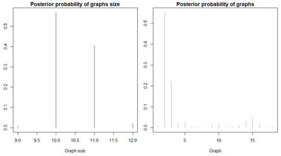
Figure 5. The figure in the left is the estimated posterior probabilities of the size of the graphs. The figure in the right is the estimated posterior probabilities of all visited graphs.

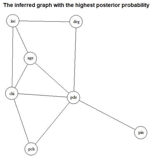
Figure 6. The figure is the inferred graph with the highest posterior probability.

The results also suggest that the respondents’ income has relationships with their own education and age. It is also shown that the income of respondents’ parents is only related to their education.

5. Computations

In this section, we aim to design an algorithm to take samples that we are interested in, such as decomposable undirected graphs, from the structural Markov graph law $\mathfrak{G}$ on $\mathfrak{U}$.

5.1. Ratio for Graph Law

Model comparison plays an important role in statistical analysis, especially in solving the problem of the ratio of distributions of variables in different states. We consider a graph itself as a random variable into the construction of this ratio between two undirected graphs $G^{\prime }$ and G, where $G^{\prime }$ is obtained from G by removing or adding one edge. This ratio can be written as

$$\mathsf{\Lambda }(G^{\prime }:G)=\frac{\pi \left(G^{\prime }\right)}{\pi \left(G\right)}.$$

The main objective of this next section is to greatly simplify this complex calculation under the assumption that the graph law $\mathfrak{G}$ is structural Markov on $\mathfrak{U}$. For the sake of convenience, we define ${\eta }_U=\pi \left(G_U\right)$ and ${\zeta }_S=\pi \left(G_S\right)$ for $U\in \mathcal{U}$ and $S\in \mathcal{S}$.

In Figure 7, it is a special case where $G^{\prime }$ is obtained from G by removing the edge $(u,v)$, which is exactly in one prime component $U\in \mathcal{U}$ of G.

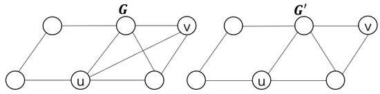
Figure 7. $G^{\prime }$ is obtained from G by removing the edge $(u,v)$.

Proposition 10. 

Let G be a fixed graph in $\mathfrak{U}$ and G has a perfect sequence $(U_1,U_2,\dots ,U_k)$ of maximal prime subgraphs. Suppose that $G^{\prime }$ is obtained from G by removing the edge $(u,v)$. Then,

1.

if u and v are contained in exactly one maximal prime subgraph $U_j$ of G, then

$$\mathsf{\Lambda }(G^{\prime }:G)=\frac{{\eta }_{U_j^{\prime }}}{{\eta }_{U_j}},j=1,2,\dots ,k;$$

2.

if u and v are contained in both two neighboring maximal prime subgraphs $U_j,U_{j+1}$ of G, then

$$\mathsf{\Lambda }(G^{\prime }:G)=\frac{{\eta }_{W^{\prime }}}{{\eta }_W},$$

(7)

where$W=U_j\cup U_{j+1}$in G.

Proof. 

See Appendix A    □

In Figure 8, it is a certain case where $G^{\prime }$ is obtained from G by adding the edge $(u,v)$ within two neighboring prime components $U_i$ and $U_j$ of G such that $u\in U_i$ and $v\in U_j$.

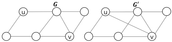
Figure 8. $G^{\prime }$ is obtained from G by adding the edge $(u,v)$.

Proposition 11. 

Let G be a fixed graph in $\mathfrak{U}$ and G has a perfect sequence $(U_1,U_2,\dots ,U_k)$ of maximal prime subgraphs. Suppose that $G^{\prime }$ is obtained from G by adding the edge $(u,v)$. Then,

1.

if u and v are contained in exactly one incomplete prime subgraph $U_h$, then

$$\mathsf{\Lambda }(G^{\prime }:G)=\frac{{\eta }_{U_h^{\prime }}}{{\eta }_{U_h}}.$$

2.

if $U_i\ni u$ and  $U_j\ni v$ are the two distinct maximal prime subgraphs of G, then there are some prime components $U_i=U_{h_1},U_{h_2},\dots ,U_{h_m}=U_j$ such that

$$\mathsf{\Lambda }(G^{\prime }:G)=\frac{{\eta }_{T^{\prime }}}{{\eta }_T},$$

(8)

where$T=U_{h_1}\cup U_{h_2}\cup \cdots \cup U_{h_m}$.

Proof. 

See Appendix A.    □

In particular, if G is a decomposable graph in $\mathfrak{U}$, then we have the following results.

Lemma 1 

([19]). Let G be a decomposable graph in $\mathfrak{U}$ and G has a perfect cliques sequence $(U_1,U_2,\dots ,U_k)$. Suppose that $G^{\prime }$ is decomposable, obtained from G by removing or adding one edge $(u,v)$. Then,

1.

If $G^{\prime }$ is obtained from G by removing the edge $(u,v)$, then u and v must belong to a clique $U_j$ of G;

2.

If $G^{\prime }$ is obtained from G by adding the edge $(u,v)$, then there exist two different cliques $U_i\ni u$ and $U_j\ni v$ such that $S=U_i\cap U_j$ is complete and separates $U_i$ and $U_j$.

Corollary 2. 

Let G be a decomposable graph in $\mathfrak{U}$ and G has a perfect cliques sequence $(U_1,U_2,\dots ,U_k)$. Suppose that $G^{\prime }$ is decomposable, obtained from G by removing or adding one edge $(u,v)$. Then,

1.

If $G^{\prime }$ is obtained from G by removing the edge $(u,v)$ within $U_j$, then

$$\mathsf{\Lambda }(G^{\prime }:G)=\frac{{\eta }_{U_u}{\eta }_{U_v}}{{\eta }_0{\eta }_U},$$

where$U_u=U_j\backslash \left\{v\right\}$,$U_v=U_j\backslash \left\{u\right\}$ and $U_0=U_j\backslash \{u,v\}$;

2.

If $G^{\prime }$ is obtained from G by adding the edge $(u,v)$ such that $u\in U_i$ and $v\in U_j$, then the ratio $\mathsf{\Lambda }(G^{\prime }:G)$ is

$$\mathsf{\Lambda }(G^{\prime }:G)=\frac{{\zeta }_S{\zeta }_{S_0}}{{\zeta }_{S_u}{\zeta }_{S_v}},$$

where$S=U_i\cap U_j$,$S_u=S\cup \left\{u\right\}$,$S_v=S\cup \left\{v\right\}$and$S_0=S\cup \{u,v\}$.

Proof. 

We first give the proof of 1. If $(u,v)\in E\left(G\right)$ and $(u,v)\notin E\left(G^{\prime }\right)$, by Lemma 1, the deleted edge $(u,v)$ must belong to a single clique $U_j$. It is worthwhile to point out that all of $U_u$, $U_v$ and $U_0$ are cliques in G and $G^{\prime }$. Then,

$${\eta }_{U_j^{\prime }}=\frac{{\eta }_{U_u}{\eta }_{U_v}}{{\eta }_{U_0}},$$

which combines with (A19) gives the result. The proof of 2 is similar.    □

5.2. Sampling Decomposable Graphs from Structural Markov Graph Laws

We now take a random graph on $\mathfrak{U}$ as the initial state to design the Markov chain Monte Carlo (MCMC) sampler for sampling from a structural Markov graph law. This technique relies on small perturbations to the edge set of a graph, indicating that one edge could be removed or added.

A reversible jump MCMC sampler is introduced for posterior sampling of decomposable graphical models, which relies on making single edge additions and removals; see [8]. We now use this jump MCMC methodology for our sample from structural Markov law in further details.

Let G denote a state variable and $G^{\prime }$ the destination variable where $G^{\prime }$ is obtained from a random graph G by removing or adding one edge, and so G would take the chain to the destination $G^{\prime }$ with probability $q(G,G^{\prime })$, which ensures detailed balance with respect to the target distribution $\pi \left(G\right)$. Then, the Metropolis–Hastings acceptance ratio can be written as

$$\alpha (G^{\prime },G)=min\left\{1,\frac{\pi \left(G^{\prime }\right)q(G^{\prime },G)}{\pi \left(G\right)q(G,G^{\prime })}\right\}.$$

(9)

In fact, the Equation (9) is not the only choice yielding detailed balance. In particular, in order to reduce the error caused by excessive proportion, we can make the following adjustment that

$$\alpha (G^{\prime },G)=min\left\{1,\frac{\pi \left(G^{\prime }\right)}{\pi \left(G\right)}\right\}\times min\left\{1,\frac{q(G^{\prime },G)}{q(G,G^{\prime })}\right\}.$$

In general, since the proposal kernel, which we will set as symmetric, that is, $q(G,G^{\prime })=q(G^{\prime },G)$. Consequently, it is indicated that the acceptance probability is only dependent on the relative densities, which will only require us to compute

$$\alpha (G^{\prime },G)=min\left\{1,\mathsf{\Lambda }(G^{\prime }:G)\right\}.$$

We randomly select a pair of vertices $u,v\in V\left(G\right)$. If $(u,v)\in E\left(G\right)$, then it is removed. If $(u,v)\notin E\left(G\right)$, then it is added. Let $G^{+(u,v)}$ denote the graph, which is obtained from G by adding the edge $(u,v)$, and similarly for $G^{-(u,v)}$. Let $G^{\left(t\right)}$ denote the state of G at time t and let ${\mathfrak{U}}^{\ast }$ be the set of decomposable undirected graphs with vertex set $V\left(G\right)$. We begin with an ER random graph as its initial state, and then a Metropolis–Hastings algorithm for sampling decomposable graphs from a structural Markov graph law $\mathfrak{G}$ can be constructed in the following Algorithm 1:

Algorithm 1 A Metropolis–Hastings algorithm for sampling decomposable graphs from a structural Markov graph law.

Input: An ER random graph $G\in \mathfrak{U}$. Output: A set of decomposable graph from $\mathfrak{U}$.     Set $G^{\left(0\right)}=G$     for  $t=0,1,2,\dots .$do          if $(u,v)\in E\left(G^{\left(t\right)}\right)$ and $G^{-(u,v)}\in {\mathfrak{U}}^{\ast }$ then               set $G^{(t+1)}=G^{-(u,v)}$ with probability $min\left(\frac{{\eta }_{U_u}{\eta }_{U_v}}{{\eta }_{U_0}{\eta }_U},1\right)$          else if $(u,v)\notin E\left(G^{\left(t\right)}\right)$ and $G^{+(u,v)}\in {\mathfrak{U}}^{\ast }$ then               set $G^{(t+1)}=G^{+(u,v)}$ with probability $min\left(\frac{{\zeta }_S{\zeta }_{S_0}}{{\zeta }_{S_u}{\zeta }_{S_v}},1\right)$          else               $G^{(t+1)}=G^{\left(t\right)}$          end if     end for     return A set of decomposable graphs.

Based on our results in Section 5.1, this algorithm implies that the acceptance probability can be obtained by only evaluating the marginal likelihood of corresponding subsets of $V\left(G\right)$ at each step when sampling from a posterior graph law in Proposition 8 or Proposition 9.

6. Conclusions

The main contribution of this paper is to define the structural Markov properties of [10] for non-decomposable undirected graphs. It is shown that an arbitrary undirected graph can be primely decomposed into the sum of several prime subgraphs. Based on the prime decomposition of undirected graphs and conditional independence, the structural Markov properties can be naturally extended to arbitrary undirected graphs.

Then, we propose a full Bayesian method for estimating the structure of a graph. This method requires that our observed data are from a certain distribution. By using our results, we have shown that the computation of posterior updating of graph law can be determined by the prime components margins, which would make the computation of the posterior graph law greatly simplified.

It should be pointed that all our research only focuses on undirected graphs. However, other classes of graphs, such as chain graphs or ancestral graphs, may have more interesting and valuable properties that can reflect the conditional independence of the graph structure in the problem of models determination. In the future, we will detail them at length.

References

- Koller, D.; Friedman, N. Probabilistic Graphical Models: Principles and Techniques; Adaptive Computation and Machine Learning; MIT Press: Cambridge, MA, USA, 2009. [Google Scholar]
- Lauritzen, S.L. Graphical Models; Oxford University Press: New York, NY, USA, 1996. [Google Scholar]
- Richardson, T. A factorization criterion for acyclic directed mixed graphs. In Proceedings of the 25th Conference on Uncertainty in Artificial Intelligence, Montreal, QC, Canada, 18–21 June 2009. [Google Scholar]
- Richardson, T.; Spirtes, P. Ancestral graph Markov models. Ann. Stat. 2002, 30, 962–1030. [Google Scholar] [CrossRef]
- Iqbal, K.; Buijsse, B.; Wirth, J. Gaussian Graphical Models Identify Networks of Dietary Intake in a German Adult Population. J. Nutr. Off. Organ Am. Inst. Nutr. 2016, 146, 646–652. [Google Scholar] [CrossRef] [PubMed]
- Larranaga, P.; Moral, S. Probabilistic graphical models in artificial intelligence. Appl. Soft Comput. 2011, 11, 1511–1528. [Google Scholar] [CrossRef]
- Verzilli, C.J.; Stallard, N.; Whittaker, J.C. Bayesian graphical models for genomewide association studies. Am. J. Hum. Genet. 2006, 79, 100–112. [Google Scholar] [CrossRef] [PubMed]
- Giudici, P.; Green, P.J. Decomposable graphical Gaussian model determination. Biometrika 1999, 86, 785–801. [Google Scholar] [CrossRef]
- Madigan, D.; Raftrey, A.E. Model selection and accounting for model uncertainty in graphical models using Occam’s window. J. Amer. Stat. Assoc. 1994, 89, 1535–1546. [Google Scholar] [CrossRef]
- Byrne, S.; Dawid, A.P. Structural Markov graph laws for Bayesian model uncertainty. Ann. Stat. 2015, 43, 1647–1681. [Google Scholar] [CrossRef]
- Li, B.C. Support condition for equivalent characterization of graph laws. Sci. Sin. Math. 2022, 52, 467–474. [Google Scholar]
- Dawid, A.P.; Lauritzen, S.L. Hyper Markov laws in the statistical analysis of decomposable graphical models. Ann. Stat. 1993, 21, 1272–1317. [Google Scholar] [CrossRef]
- Green, P.J.; Thomas, A. A structural Markov property for decomposable graph laws that allows control of clique intersections. Biometrika 2018, 105, 19–29. [Google Scholar] [CrossRef]
- Leimer, H.G. Optimal decomposition by clique separators. Discret. Math. 1993, 113, 99–123. [Google Scholar] [CrossRef]
- Dawid, A.P. Conditional independence in statistical theory. J. R. Stat. Soc. B. 1979, 41, 1–15. [Google Scholar] [CrossRef]
- Dawid, A.P. Conditional independence for statistical operations. Ann. Stat. 1980, 8, 598–617. [Google Scholar] [CrossRef]
- Meek, C. Strong Completeness and Faithfulness in Bayesian Networks; Morgan Kaufmann: San Francisco, CA, USA, 1995. [Google Scholar]
- Hoff, P.D. Extending the rank likelihood for semiparametric copula estimation. Ann. Appl. Stat. 2007, 23, 103–122. [Google Scholar]
- Frydennberg, M.; Lauritzen, S.L. Decomposition of maximum likelihood in mixed graphical interaction models. Biometrika 1989, 76, 539–555. [Google Scholar] [CrossRef]
- Asmussen, S.; Edwards, D. Collapsibility and response variables in contingency tables. Biometrika 1983, 70, 567–578. [Google Scholar] [CrossRef]
- Wang, X.F.; Guo, J.H. Junction trees of general graphs. Front. Math. China 2008, 3, 399–413. [Google Scholar] [CrossRef]
Disclaimer/Publisher’s Note: The statements, opinions and data contained in all publications are solely those of the individual author(s) and contributor(s) and not of MDPI and/or the editor(s). MDPI and/or the editor(s) disclaim responsibility for any injury to people or property resulting from any ideas, methods, instructions or products referred to in the content. |
© 2023 by the authors. Licensee MDPI, Basel, Switzerland. This article is an open access article distributed under the terms and conditions of the Creative Commons Attribution (CC BY) license (https://creativecommons.org/licenses/by/4.0/).