Abstract
Continuous probability distributions can handle and express different data within the modeling process. Continuous probability distributions can be used in the disclosure and evaluation of risks through a set of well-known basic risk indicators. In this work, a new compound continuous probability extension of the reciprocal Rayleigh distribution is introduced for data modeling and risk analysis. Some of its properties including are derived. The estimation of the parameters is carried out via different techniques. Bayesian estimations are computed under gamma and normal prior. The performance and assessment of all techniques are studied and assessed through Monte Carlo experiments of simulations and two real-life datasets for applications. Two applications to real datasets are provided for comparing the new model with other competitive models and to illustrate the importance of the proposed model via the maximum likelihood technique. Numerical analysis for expected value, variance, skewness, and kurtosis are given. Five key risk indicators are defined and analyzed under Bayesian and non-Bayesian estimation. An extensive analytical study that investigated the capacity to reveal actuarial hazards used a wide range of well-known models to examine actuarial disclosure models. Using actuarial data, actuarial hazards were evaluated and rated.
Keywords:
actuarial risks analysis; asymmetric actuarial data; insurance-claims; likelihood; value-at-risk; reciprocal rayleigh MSC:
60E05; 62H05; 62E10; 62F10; 62F15; 62P05
1. Introduction
Actuarial science is a mathematical branch that deals with the financial consequences of uncertain future events. It employs statistical and mathematical methods to evaluate and manage risks in the finance and insurance industries. Actuaries use probability distributions to model and measure the likelihood of different outcomes and determine the anticipated future losses. Probability distribution is a function that describes the probability of different outcomes for a random variable. Actuaries utilize various probability distributions, such as Poisson, normal, exponential, and log-normal, to model diverse types of risks, including morbidity, mortality, and property damage, based on the nature of the risk being modeled and the data available for the modeling. Actuaries use probability distributions to compute the expected future losses, which are used to set insurance premiums, design insurance products, and assess investment strategies. Actuaries also use simulation techniques to test their models and evaluate the financial results of insurance policies and investments under various scenarios.
The adequacy of probability-based distributions in describing risk exposure is a common practice in the field of risk management. Typically, risk exposure statistics are defined by one or a small group of numbers that are functions of a specific model, commonly referred to as key risk indicators (KRIs) (Lane [1]; Klugman et al. [2]). These KRIs provide actuaries and risk managers with valuable information about a company’s exposure to specific types of risk. Several KRIs, including value-at-risk (VARK), tail-value-at-risk (TVARK) or conditional tail expectation (CTE), conditional-value-at-risk (CVARK), tail variance (TV), mean excess loss (MEL), and tail mean-variance (TMV), have been developed and can be analyzed (Shrahili et al. [3]; Mohamed [4]). In particular, VARK is commonly used to estimate the quantile distribution of aggregate losses. Actuaries and risk managers focus on calculating the probability of a bad outcome, measured by the VARK indicator at a specific probability or confidence level. This indicator is used to estimate the amount of capital required to manage potential unfavorable events. The ability of an insurance company to handle such situations is highly valued by actuaries, authorities, investors, and rating agencies (Wirch [5]; Artzner [6]; Tasche [7]; Acerbi [8]; Landsman [9]; Furman and Landsman [10]). In summary, probability-based distributions and KRIs are essential tools for evaluating risk exposure in companies. The use of such indicators is widespread, and the ability to manage risk effectively is highly valued in the field of risk management.
For the left-skewed insurance-claims data, this work suggests certain KRI variables, such as VARK, TVARK, TV, MEL, and TMV, using a new model termed the exponentiated generalized reciprocal Rayleigh Poisson (EGRRP) distribution. Statistical methods frequently employed in actuarial risk analysis include:
- Actuaries employ probability distributions to simulate the possibility of a variety of events, including claims, fatalities, and policy cancellations. The Poisson distribution, the exponential distribution, and the Weibull distribution are frequently used distributions in actuarial science.
- Modeling the time until a specific event, such as a death or policy cancellation, is conducted using survival analysis. This method is employed to compute life expectancy and assess the likelihood of survival for a specific time period.
- Modeling with stochastic processes: stochastic modeling is used to simulate unpredictable events such as insurance-claims and policy cancellations. This method is employed to compute the variability of these estimations and to estimate the expected value of upcoming claims.
- Loss distributions: Loss distributions are used to simulate how losses are distributed as a result of things such as claims and insurance cancellations. The estimated value of potential losses is calculated using this method, and the risk involved with such losses is also identified.
- Actuaries employ statistical approaches, such as portfolio optimization and hedging strategies, to evaluate and manage financial risks.
The Reciprocal Rayleigh (RR), also known as the inverse Rayleigh distribution, is an important probability distribution that is widely used in many fields, including reliability engineering, signal processing, and wireless communications. The RR distribution is a flexible distribution that can model a wide range of phenomena. It is a continuous distribution with support on the positive real line, and it has two parameters that control the location and scale of the distribution. The RR distribution can be used to model data that are positively skewed and have long tails, which are common in many real-world applications. The RR distribution is commonly used in reliability engineering to model the lifetime of a system or component. In this context, the RR distribution is used to model the time until failure, and it has been shown to provide a good fit to many types of failure data. The RR distribution is used in signal processing to model the amplitude of a random signal. In this context, the RR distribution is used to model the probability density function of the envelope of a narrowband Gaussian noise signal, which is commonly used in wireless communications. The RR distribution is used in statistical inference to model the distribution of the inverse of a random variable. In this context, the RR distribution is used to model the distribution of the ratio of two independent Rayleigh-distributed random variables, which is commonly used in wireless communications and signal processing.
The RR distribution is used in reliability engineering to model the lifetime of a system or component. In this context, the RR distribution is used to model the time until failure, and it has been shown to provide a good fit to many types of failure data. The RR distribution has also been used in finance to model the distribution of returns on investment portfolios. In this context, the RR distribution can be used to model the distribution of the inverse of returns, which can be useful in portfolio risk management. Overall, the RR distribution has a wide range of applications in many fields, including reliability engineering, wireless communications, signal processing, statistical inference, and finance. Its flexibility, reliability modeling capabilities, and usefulness in modeling the distribution of the inverse of a random variable make it a valuable tool for researchers and practitioners in many different areas.
The RR distribution can be used to model the distribution of losses in insurance-claims. This is useful in estimating the risk of losses and setting premiums. It can also be used to model the risk of many events in insurance, such as natural disasters or accidents. This can help insurance companies to better understand and manage their risk exposure. Moreover, the RR distribution can be used to model the behavior of policyholders in insurance, such as the frequency and severity of claims. This can help insurance companies to design policies that are better suited to their customers’ needs. Finally, the RR distribution can be used in actuarial modeling to estimate the probability of future events based on historical data. This is useful in predicting the likelihood of future claims and setting reserves. Overall, the RR distribution has several applications in actuarial sciences and insurance. Its flexibility and usefulness in modeling the distribution of losses and risk make it a valuable tool for insurance companies and actuaries. The RR distribution, also known as the inverse Rayleigh (IR) distribution, has several applications in actuarial sciences and insurance. The RR distribution is considered as a distribution for a lifetime random variable (r.v.). The probability density function (PDF) and cumulative distribution function (CDF) of the RR model are given by
and
respectively, where . The exponentiated-generalized-Poisson (EGP) family of distributions is a new flexible compound family of distributions that Aryal and Yousof [11] introduced and explored. The EGP family’s CDF and PDF are provided by:
and
respectively, where , and . For we have the exponentiated-G Poisson (EGP) class of distribution, and for we have the generalized Poisson (GP) class of distribution, both of which are embedded in EGP class. Since (2) refers to the baseline CDF of the RR model and (3) refers to the baseline CDF of the EGP family, then, substituting (2) in (3), we derive a new compound RR distribution called EGRRP with CDF which can be expressed as
where , , and The corresponding PDF can be written as
Figure 1 illustrates that the PDF of the EGRRP model may exhibit various shapes, such as right-skewed, left-skewed, and unimodal. On the other hand, Figure 2 shows that the hazard rate function (HRF) of the EGRRP model may be decreasing and upside down. Moreover, there are several notable extensions of the RR distribution, including Voda [12], Mukerjee and Saran [13], Nadarajah and Kotz [14], Nadarajah and Gupta [15], Barreto-Souza et al. [16], Krishna et al. [17], Mahmoud and Mandouh [18], Mead et al. [19], Chakraborty et al. [20], and Cordeiro et al. [21], among others.
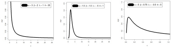
Figure 1.
Graphs of the EGRRP PDF for selected parameter values.
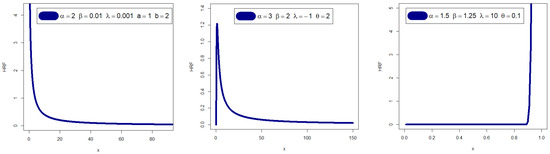
Figure 2.
Graphs of the EGRRP HRF for selected parameter values.
2. Properties and Numerical Analysis
Using the power series expansion of the PDF in (6) can be expressed as
Using
the last equation of can be expressed as
where
and is the RR density with scale parameter . By integrating (7), we obtain another simple results of as where is the CDF of the RR distribution with scale parameter . The rth ordinary moment of is given by Using (7), we obtain
where and Setting in (8), we have the mean of as . We can find the MGF, say by
The sth incomplete moments, say is given by Using (7), we obtain
where
and The th probability weighted moments (PWMs) of following the EGRRP model, say , is formally defined by Using Equations (5) and (6), we can write where
Then, the th PWM of can be obtained and summarized as
The th moment of the residual life, say uniquely determine Therefore
where and . The th moment of the reversed residual life, say . Therefore
where Table 1 lists a few sub models from the EGRRP model. A numerical investigation of the E(X), Variance (V(X)), skewness (Ske(X)), and kurtosis (Ku(X)) is shown in Table 2. According to Table 2, the proposed model’s skewness can have both positive and negative values. The proposed model’s kurtosis ranges from greater than three to fewer than three.

Table 1.
Some sub models from the EGRRP model.
Table 2.
E(X), VARK(X), Ske(X), and Ku(X) of the EGRRP distribution.
3. Actuarial Indicators for Risk Analysis and Management
A specific insurance policy or the insurance sector as a whole may be affected by future occurrences, and risk analysis in insurance data refers to the process of assessing and estimating the chance of such events. Identification, evaluation, and development of solutions to control or mitigate potential risks are the objectives of risk analysis. To ascertain the degree of risk associated with a certain policy or portfolio of policies, this procedure entails gathering, evaluating, and interpreting data regarding a variety of elements, including demographic data, insurance-claims history, and economic indicators. Insurance firms use the findings of risk analysis to determine rates, make underwriting judgements, and create loss mitigation plans. KRIs are an essential tool for risk management as they provide a clear, quantifiable, and actionable measure of an organization’s key risks, allowing organizations to take proactive steps to manage these risks and avoid negative consequences. The selection of KRIs is important and should be based on the specific risks faced by the organization and its overall risk management strategy.
3.1. VARK Indicator
The VARK, a widely utilized financial term, is a measure of the maximum expected loss that a portfolio or investment may incur over a given time period and is commonly employed as a risk management tool by financial institutions to assess market risk. This single-number indicator provides a concise summary of the potential loss of a portfolio or investment. For example, a portfolio with a VARK of USD 1 million at a 95% confidence level implies a 5% probability that the portfolio will experience a loss exceeding USD 1 million during the specified time frame. Risk exposure is an inevitable aspect of the operations of insurance organizations, and actuaries have developed Various risk indicators to statistically evaluate it. VARK is used to determine the most probable maximum amount of capital that might be lost over a specified duration. However, a loss that is unbounded or at least equal to the value of the portfolio is not necessarily informative. The risk profiles of different portfolios with the same maximum loss can vary substantially. Therefore, the VARK typically depends on the probability distribution of the loss random variable, which is influenced by the overall distribution of the risk factors that affect the portfolio. Then, for EGRRP distributions, we can simply write
The refers to the quantile of the EGRRP model. The VARK is a practical instrument for risk management since it gives a clear and succinct assessment of the potential loss of an investment or portfolio. It has drawbacks, too, as it simply offers a point estimate of the probable loss and ignores tail risks or extreme events. Financial organizations frequently combine VARK with other risk management tools such as stress testing and scenario analysis to address these constraints.
3.2. TVARK Risk Indicator
The at the confidence level, can be defined as the expected losses given that the losses exceed the of the distribution of . Then, the TVARK() can be then calculated as
Then, we have
So, can be calculated as average all the values over the confidence level . That means that the indicator of gives us many more information about the tail of the EGRRP distribution and its properties. Generally, the can also be written as
where is the MEL function evaluated at the quantile.
3.3. The TV Indicator
The TV indicator (TV ()) can be expressed as
For the EGRRP model, the quantity is not exist; however, we dealt with this amount using numerical techniques to find the closest possible value for it. It is known that numerical techniques represent the best solution in many of the problems of estimation and specialist modeling, where is given in (13).
3.4. TMV Risk Indicator
The TMV risk indicator (TMV ()) for the EGRRP model can then be derived as
Then, for any loss random variable, , and for the Some other common examples of KRSIs can be mentioned such as:
- Indicators of the frequency and size of losses resulting from different risks, including accidents, losses from fraud, or losses from natural catastrophes, are measured by these KRSIs.
- Volatility indicators: These KRSIs measure the level of volatility in various financial markets, such as the stock market, currency market, or commodities market.
- Credit risk indicators: These KRSIs measure the credit risk of various borrowers, such as individuals or organizations, based on their credit history and financial information.
- Operational risk indicators: These KRSIs measure the level of operational risk associated with various processes, such as supply chain disruptions, IT failures, or human errors.
- Market risk indicators: These KRSIs measure the level of market risk associated with investments, such as stocks, bonds, or commodities.
4. Estimation
4.1. Classical Estimation
4.1.1. Maximum Likelihood Technique
For determining the maximum likelihood estimation (MLE) of , we formulate the log-likelihood function as follows
The components of the score vector components are easily derived and then solved. To solve these equations, it is usually more convenient to use nonlinear optimization techniques such as the quasi-Newton algorithm to numerically maximize . A popular numerical optimization approach for maximizing functions is the quasi-Newton algorithm. It is an iterative approach that computes the search direction at each iteration using approximations of the Hessian matrix. The fundamental goal of the quasi-Newton approach is to update a Hessian matrix approximation based on gradient data gathered from evaluating the objective function at various locations. Using the updated Hessian approximation, the technique determines a search direction at each iteration and moves in that direction to find a new location to evaluate the objective function. The Broyden–Fletcher–Goldfarb–Shanno (BFGS) algorithm is the most used quasi-Newton algorithm. The rank-two update formula used by the BFGS algorithm to update the Hessian approximation is made to keep the approximation’s positive definiteness. When there are many variables in an optimization issue, the BFGS algorithm is frequently used.
4.1.2. Bootstrapping Technique
The bootstrapping technique is a potent statistical technique, particularly useful when dealing with small sample sizes. In traditional scenarios, assuming a normal or t-distribution is not feasible when working with less than 40 samples. However, bootstrap techniques are well-suited for sample sizes of less than 40 as they involve resampling and do not make any assumptions about the data distribution. With the increasing availability of computing resources, bootstrapping has gained popularity as a practical approach that requires the use of a computer. The following section will illustrate how this technique operates. This is due to the necessity of using a computer for bootstrapping to be useful. In the section that follows, we will examine how these function. There are several different types of bootstrapping techniques, including:
- Non-parametric bootstrapping: In non-parametric bootstrapping, the statistic of interest is calculated directly from the resampled data without making any assumptions about the underlying probability distribution. This is the most commonly used type of bootstrapping and can be used for a wide range of estimators.
- Parametric bootstrapping: In parametric bootstrapping, the resampled data are generated from a specific parametric distribution that is assumed to describe the data. This can be useful when the underlying distribution is known or can be reasonably assumed and can lead to more accurate estimates than non-parametric bootstrapping.
- Bootstrap aggregating (bagging): In bagging, multiple copies of the original dataset are created by resampling, and then a separate model is trained on each of these new datasets. The final estimate is then obtained by averaging the estimates of the individual models. Bagging is commonly used in machine learning and can improve the accuracy and stability of models that are prone to overfitting.
- Cross-validation bootstrapping: In cross-validation bootstrapping, the original dataset is divided into several subsets, and then a separate model is trained on each subset while using the remaining data for validation. The final estimate is then obtained by averaging the estimates of the individual models. Cross-validation bootstrapping is commonly used in machine learning and can help to prevent overfitting by reducing the variance of the estimate.
- Bootstrapping has become a widely used technique for statistical inference and estimation, and it has been applied to a wide range of fields, including finance, engineering, social sciences, and natural sciences. Bootstrapping can be implemented using various statistical software packages, including R, Python, MATLAB, and SAS.
4.1.3. Technique of Cramér–von Mises
The Cramér–von Mises estimation (CVME) technique of the parameters is based on the theory of minimum distance estimation. The CVME of the parameters , , , and are obtained by minimizing the following expression with respect to the parameters , , , and , respectively, where
where and
Then, CVME of the parameters are obtained by solving the following non-linear equations
and
where , and are the values of the first derivatives of the CDF of EGRRP distribution with respect to , respectively.
4.2. Bayesian Estimation
In this part, we build estimators for the EGRRP distribution’s unknown parameters using Bayesian techniques. The maximum likelihood estimator frequently fails to converge, particularly in models with larger dimensions. In these situations, Bayesian approaches are sought after. Bayesian approaches initially appear to be highly complicated because the estimators entail unsolvable integrals. Here we assume the gamma priors of the parameters of the following forms
where, Gamma stands for gamma distribution with shape parameter and scale parameter , and normal stands for the normal distribution with shape parameter and
The Gamma distribution is a conjugate prior for several common likelihood functions, including the Poisson, exponential, and normal distributions. This means that if we choose a Gamma prior, the resulting posterior distribution will also be a Gamma distribution. This makes the Bayesian inference computationally efficient and enables us to obtain the posterior distribution in closed form. The Gamma distribution is a distribution over positive values only, which makes it a natural choice for modeling quantities that are inherently positive, such as rates, counts, or durations. The Gamma distribution is a flexible distribution that can take on a wide range of shapes, including skewed, unimodal, and multimodal shapes. This makes it a good choice for modeling a wide range of different data types. The parameters of the Gamma distribution have clear and intuitive interpretations, which makes it easy to incorporate prior knowledge into the model. For example, the shape parameter of the Gamma distribution can be interpreted as the number of prior observations, and the scale parameter can be interpreted as the prior sum of the observations. The Gamma distribution is relatively robust to deviations from the assumed model, which makes it a good choice when the data are noisy or when there is uncertainty about the model specification.
It is further assumed that the parameters are to be independently distributed. The joint prior distribution is given by
The posterior distribution of the parameters is defined by As a consequence, we recommend employing Markov chain Monte Carlo (MCMC) methods, particularly the Gibbs sampler and the Metropolis Hastings (MH) technique. We implemented a hybrid MCMC approach to draw samples from the joint posterior of the parameters because it is not possible to collect the conditional posteriors of the parameters in any basic structures. To implement the Gibbs algorithm, the full conditional posteriors of , , , and are given by
where
The simulation algorithm we followed is given by
- 1.
- Provide the initial values, say , , , and where and (the initial values are randomly determined by the selection of the researcher, provided that it is within the specified range) then at stage;
- 2.
- Using MH algorithm, generate ;
- 3.
- Then, using the well-known algorithm MH, generate ;
- 4.
- Then, using the well-known algorithm MH, generate ;
- 5.
- Then, using the well-known algorithm MH, generate ;
- 6.
- Repeat steps , times to obtain the samples of size from the corresponding posteriors of interest.
Obtain the Bayesian estimates of and using the following formulae where is the burn-in period of the generated Markov chains.
5. Simulations for Comparing Bayesian and Classical Approaches
Simulation studies are a crucial tool for assessing and contrasting various statistical techniques, including traditional estimation techniques. In simulation studies, data are generated based on a given model, and the efficacy of various estimating techniques is evaluated using the generated data. We shall talk about the value of simulation studies for contrasting traditional estimating techniques in this essay. Simulations are an important tool for comparing Bayesian and classical estimation techniques because they allow us to systematically evaluate the performance of different techniques under a wide range of conditions. Simulations allow us to examine the performance of Bayesian and classical techniques under different sample sizes, which can be particularly useful when the sample size is small. By simulating data with different sample sizes, we can assess how well the different techniques perform under conditions of low data availability. Simulations allow us to evaluate the performance of Bayesian and classical techniques under different parameter values, which can be important when the parameters of interest are not known a priori. By simulating data with different parameter values, we can assess how well the different techniques perform under conditions of parameter uncertainty. Simulations allow us to evaluate the robustness of Bayesian and classical techniques to deviations from the assumed model. By simulating data that deviate from the assumed model, we can assess how well the different techniques perform under conditions of model misspecification. Simulations allow us to compare the accuracy and precision of Bayesian and classical techniques under different conditions. By simulating data with known parameter values, we can assess how accurately and precisely the different techniques estimate the true parameters. Simulations allow us to assess the computational efficiency of Bayesian and classical techniques under different conditions. By simulating data with different sample sizes and parameter values, we can assess how well the different techniques scale to larger and more complex datasets.
The mean squared error (MSE) is a performance indicator that is frequently used in simulation studies to assess the precision of a statistical model or estimator. The average of the squared discrepancies between the estimated values and the actual values of the parameter being estimated is known as the MSE. In simulation research, MSE is chosen over measures of dispersion and biases for a number of reasons. It is a thorough evaluation. The MSE accounts for both the estimator’s bias and variability. Measurements of bias simply reflect the discrepancy between the estimator and the true value, while measures of dispersion, such as variance or standard deviation, only record the estimator’s variability. Because it takes into account both types of error, the MSE offers a more complete evaluation of the estimator’s performance. It is simple to understand. The MSE is simple to read because it uses the same units as the parameter being estimated.
A MCMC simulation study is conducted and performed in this section to assess and compare the performance of the different estimators of the unknown parameters of the EGRRP distribution. This performance is assessed using the average values (AVs) of estimates and the MSEs. First, we generated samples of the EGRRP distribution, where and choosing
The tables present the AVs and MSEs of various parameter estimators, namely MLEs, Bootstrap, CVMEs, and Bayesian estimators. To evaluate the Bayesian estimators, the MCMC technique is used with a flexible gamma prior under the SELF for all parameters, except for parameter λ, which uses a normal prior. Hyperparameters are assumed to be known and selected to have a prior mean equal to the initial value and a prior variance of one. Results from Table 3, Table 4, Table 5 and Table 6 demonstrate that all estimators exhibit consistency, as evidenced by the decreasing MSEs as the sample size increases. Moreover, the Bayesian estimators have lower MSEs than the other estimators, and in some cases, the MSEs of the Bayesian and MLEs are very similar. The computations in this section were performed using the Mathcad program, version 15.0.
Table 3.
The results of the AVs and their corresponding MSEs (in parentheses) for .
Table 4.
The results of the AVs and their corresponding MSEs (in parentheses) for .
Table 5.
The results of the AVs and their corresponding MSEs (in parentheses) for .
Table 6.
The results of the AVs and their corresponding MSEs (in parentheses) for .
6. Applications for Comparing Bayesian and Classical Estimations
Two real-life datasets for applications are introduced and analyzed to for some purposed including comparing Bayesian and classical estimations. In these applications, we recommend and consider the Cramér–von Mises (), the Anderson–Darling () and the Kolmogorov–Smirnov (KS) test statistic for comparing methods. The 1st dataset consists of 100 observations of breaking stress of carbon fibers (see Nichols and Padgett [22]). Table 7 gives the values of estimators of , and , the KS test statistics and its p-value, and and for all techniques using the 1st dataset. From Table 7 we conclude that the Bayesian technique is the best technique with KS = , p-value = , = , and = . However, all other techniques performed well. For the 2nd dataset (see Smith and Naylor [23]), these data were originally obtained by workers at the UK National Physical Laboratory. Table 8 gives the values of estimators of , and , the KS test statistics and its p-value, and and for all techniques using the 2nd dataset. From Table 8 we conclude all other techniques performed well, and according to these results we cannot select a technique as the best one.
Table 7.
The estimated parameters, KS, p-values, , and for all estimation techniques using the 1st dataset.
Table 8.
The estimated parameters, KS, p-values, , and for all estimation techniques using the 2nd dataset.
7. Applications for Comparing Competitive Distributions
This section presents two real-life applications of demonstrating the EGRRP distribution using real datasets. We compare the results of the new EGRRP distribution with the Weibull-inverse-Weibull (WIW), exponentiated-inverse-Weibull (EIW) (see Nadarajah and Kotz [14]), Kumaraswamy-inverse-Weibull (KumIW) (see Mead and Abd-Eltawab [19]), beta-inverse-Weibull (BIW) (Barreto-Souza et al. [16]), transmuted-inverse-Weibull (TIW) (see Mahmoud and Mandouh [18]), gamma extended-inverse-Weibull (see GEIW) (Silva et al. [24]), Marshall-Olkin-inverse-Weibull (MOIW) (see Krishna et al. [17]), and Reciprocal Weibull (RW) distributions.
The unknown parameters of these PDFs are all positive real numbers, except for the TIW distribution. To compare the distributions, we use various criteria such as the maximized Log-Likelihood, AIC (Akaike Information Criterion), CAIC (Consistent Akaike Information Criterion), BIC (Bayesian Information Criterion), and HQIC (Hannan–Quinn Information Criterion). All computations are conducted using the R PROGRAM. Additionally, the TTT graph is used to graphically verify whether the data can be fit to a specific distribution or not, which is an important graphical approach (Aarset [25]). A straight diagonal TTT graph indicates a constant HRF; a concave TTT graph indicates an increasing (or decreasing) HRF; and a U-shaped (bathtub) TTT graph indicates a unimodal HRF, while other shapes indicate otherwise. The TTT graphs for the two real datasets are presented in Figure 3, where we conclude that the empirical HRFs of the two datasets are increasing.
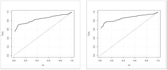
Figure 3.
TTT plot for breaking stress of carbon fibers (left) and TTT plot for the strengths data of the glass fibers (right).
We contrast the EGRRP model with strong competitive distributions in Table 9, Table 10, Table 11 and Table 12. Table 9 gives −2ℓ, AIC, BIC, HQIC, and CAIC for the 1st dataset. Table 10 lists MLEs and their standard errors (in parentheses) for the 1st dataset. Table 11 gives −2ℓ, AIC, BIC, HQIC, and CAIC for the 2nd dataset. Table 12 lists MLEs and their standard errors (in parentheses) for the 2nd dataset. Of all models fitted to the two real-life datasets, the EGRRP model provides the best values for the AIC, BIC, HQIC, and CAIC statistics. So, it may be picked as the best option. For the first set of data, Figure 4 shows graphs for estimated CDFs, estimated PDFs, P-P graph, and the Kaplan–Meier graph. The graphs of estimated CDFs estimated PDFs, P-P graph, and the Kaplan–Meier survival graph for the second dataset are shown in Figure 5. These graphs suggest that for both datasets, the suggested distribution provides a better match than other non-nested and nested distributions.
Table 9.
−2ℓ, AIC, BIC, HQIC, and CAIC for the 1st dataset.
Table 10.
MLEs and their standard errors (in parentheses) for the 1st dataset.
Table 11.
−2ℓ, AIC, BIC, HQIC, and CAIC for the 2nd dataset.
Table 12.
MLEs and their standard errors for the 2nd dataset.
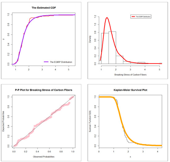
Figure 4.
Estimated CDF (top left), estimated PDF (top right), P-P graph (bottom left), and Kaplan–Meier survival (bottom right) for the 1st dataset.
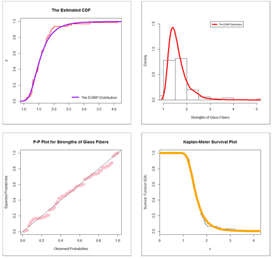
Figure 5.
Estimated CDF (top left), estimated PDF (top right), P-P graph (bottom left), and Kaplan–Meier survival (bottom right) for the 2nd dataset.
8. Risk Analysis for Insurance-Claims Data
In insurance data analysis, the temporal growth of claims over time for each relevant exposure period is often presented in a triangle format. The exposure period can refer to the year the insurance policy was purchased or the time frame in which the loss occurred. It should be noted that the origin period need not be annual and can be monthly or quarterly. The claim age or claim lag is the duration between the origin period and when the claim is made. To identify consistent trends, division levels, or risks, data from various insurance policies are often combined. In this study, we utilize a U.K. Motor Non-Comprehensive account as an example of an insurance-claims payment triangle. For convenience, we set the origin period between 2007 and 2013 (see Shrahili et al. [3]; Mohamed [4]). The claims data are presented in an insurance-claims payment data frame in a standard database format, with the first column listing the development year, the incremental payments, and the origin year spanning from 2007 to 2013. It is crucial to note that a probability-based distribution was initially used to analyze this insurance-claims data. The data are analyzed using numerical and graphical techniques. The numerical approach involves fitting theoretical distributions such as the normal, uniform, exponential, logistic, beta, lognormal, and Weibull distributions. These distributions are then examined using graphical tools such as the skewness-kurtosis graph (or the Cullen and Frey graph) (see Figure 6). Figure 6 shows that our data are left-skewed and have a kurtosis of less than three.
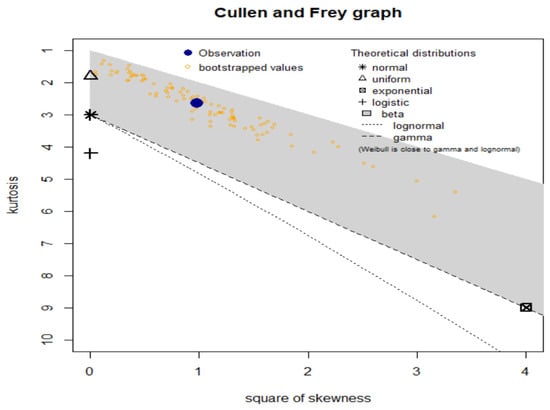
Figure 6.
Cullen-Frey graph for the actuarial claims data.
Different approaches are utilized to examine multiple aspects of the insurance-claims data, which are presented in Figure 7. The NKDE method is implemented to analyze the initial shape of the insurance-claims density, while the Q-Q graph is used to evaluate the normality of the data. The TTT graph is employed to assess the initial shape of the empirical HRF, and the “box graph” is utilized to identify explanatory variables.
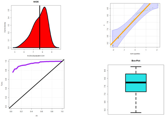
Figure 7.
The NKDE graph (top left graph), the Q-Q graph (top right graph), the TTT graph (bottom left graph), and the box graph (bottom right graph) for the claims data.
Figure 7 displays the results of the various graphs. The initial density is demonstrated to be an asymmetric function with a left tail in the top left graph. The bottom right graph indicates that there are no extreme claims. The bottom left graph shows that the HRF for models explaining the data should have a monotonically increasing trend. Scattergrams for the insurance-claims data are presented in Figure 8. The autocorrelation function (ACF) and partial autocorrelation function (partial ACF) for the data are depicted in Figure 9.
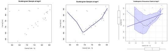
Figure 8.
The initial scattergram (left graph), the fitted scattergram (middle graph), and smoothed scattergram (right graph).
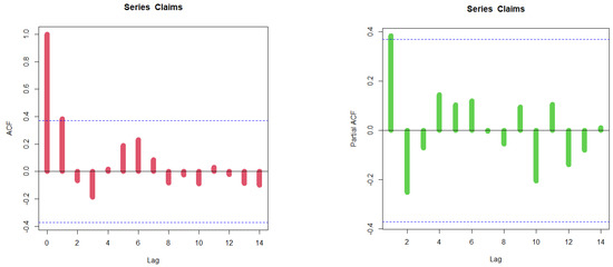
Figure 9.
The ACF (left graph), and the partial ACF (right graph) for the insurance-claims data.
To assess risk for the insurance-claims data, measures such as VARK, TVARK, TV, TMV, and MEL are employed at various confidence levels, which are listed in Table 13. Table 14 gives the estimated parameters for the EGRRP under insurance-claims data. Table 15 lists the results of the KRIs for the IR under insurance-claims data. Table 16 gives the estimated parameters for the IR under insurance-claims data. The EGRRP and RR distributions are compared using five measures, while the KRIs for the EGRRP and IR are listed in Table 13 and Table 15, respectively. Table 14 provides the estimators and ranks for the EGRRP model under the claims data for all estimation methods, while Table 16 lists the KRIs for the RR distribution under the claims data for all estimation methods. The RR distribution is chosen as the baseline distribution for comparison with the new EGRRP distribution. Based on these tables, the following results can be highlighted:
Table 13.
The results of the EGRRP under insurance-claims data.
Table 14.
The estimated parameters for the EGRRP under insurance-claims data.
Table 15.
The results of the KRIs for the IR under insurance-claims data.
Table 16.
The estimated parameters for the IR under insurance-claims data.
- For all risk assessment Bayesian and non-Bayesian techniques |:
- For all risk assessment Bayesian and non-Bayesian techniques |:
- For most risk assessment techniques |:
- For all risk assessment techniques |:
- For all risk assessment Bayesian and non-Bayesian techniques |:
- Under the EGRRP model and the MLE technique: The VARK() is a consistently growing indicator which starts with 2602.272196 and terminates with 145,993.327739; the TVARK() is a consistently growing indicator which starts with 7534.159674 and terminates with 65,808.922847. However, the TV(), the TMV(), and the MEL() are monotonously reducing.
- Under the RR distribution and the MLE technique: The VARK() is a consistently growing indicator which starts with 1628.234966 and terminates with 36,791.27132; the TVARK() is a consistently growing indicator which starts with 3547.122526 and terminates with 73,594.813549; the TV(), the TMV(), and the MEL() are monotonously reducing indicators.
- Under the EGRRP model and the bootstrapping technique: The VARK() is a consistently growing indicator which starts with 2832.283001 and terminates with 123,576.386617; the TVARK() is a consistently growing indicator which starts with 7560.430006 and terminates with 84,874.267755. However, the TV(), the TMV(), and the MEL() are monotonously reducing.
- Under the RR distribution and the OLSE technique: The VARK() is a consistently growing indicator which starts with 1692.496862 and terminates with 38,243.320243; the TVARK() is a consistently growing indicator which starts with 3687.117754 and terminates with 76,499.395591. Additionally, the TV (), the TMV (), and the MEL() are monotonously reducing indicators.
- Under the EGRRP model and the CVM technique: The VARK() is a consistently growing indicator which starts with 2770.998013 and terminates with 123,130.65901; the TVARK() is a consistently growing indicator which starts with 7453.230383 and terminates with 84,870.02498. However, the TV(), the TMV(), and the MEL() are monotonously reducing.
- Under the RR distribution and the CVM technique: The VARK() is a consistently growing indicator which starts with 2635.229755 and terminates with 59545.123954; the TVARK() is a consistently growing indicator which starts with 5740.868751 and terminates with 119,110.108205. However, the TV(), the TMV(), and the MEL() are monotonously reducing indicators.
- Under the EGRRP model and the Bayesian technique: The VARK() is a consistently growing indicator which starts with 2463.713921 and terminates with 129,788.635; the TVARK() is a consistently growing indicator which starts with 6896.600374 and terminates with 28,585.213639. However, the TV(), the TMV(), and the MEL() are monotonously reducing.
- Under the RR distribution and the Bayesian technique: The VARK() is a consistently growing indicator which starts with 1628.247409 and terminates with 36,791.552475; the TVARK() is a consistently growing indicator which starts with 3547.149632 and terminates with 73,595.375934; the TV(), the TMV(), and the MEL() are monotonously reducing indicators.
- For the EGRRP model and its corresponding RR base line model, the Bayesian approach is recommended since it offers the most acceptable risk exposure analysis.
9. Conclusions
Probability-based distributions are used by actuaries to determine the expected values of unexpected risk, which are then used to determine insurance premiums, create insurance products, and assess investment plans. Actuaries also employ simulation tools to test their algorithms and assess how different scenarios may affect the financial results of investments and insurance policies. Probability-based distributions can be used to explain risk exposure, often expressed as one or a few key risk indicators derived from a specific probability model. These indicators provide valuable insights for actuaries and risk managers to understand a company’s exposure to various types of risks, such as value-at-risk, tail-value-at-risk, conditional value-at-risk, tail variance, mean excess loss, and tail mean-variance. Different types of data can be analyzed using probability distributions in the modeling process. A new extension of the Reciprocal Rayleigh distribution is introduced and analyzed, including properties such as moments, incomplete moments, probability-weighted moments, moment generating function, residual life, and reversed residual life functions. Parameter estimation is performed through various techniques, including Bayesian estimators under gamma and normal priors using the squared error loss function. The performance of all estimation techniques is evaluated through Monte Carlo simulations and two real data applications. These applications compare the new model with other competitive models and demonstrate the importance of the proposed model via the maximum likelihood technique. Numerical analysis for expected value, variance, skewness, and kurtosis is provided. An extensive analytical study is conducted to evaluate and rate actuarial hazards using a wide range of well-known models for actuarial disclosure. Actuarial data are used to reveal and assess these hazards.
Based on risk analysis, the following results can be highlighted:
- For all risk assessment Bayesian and non-Bayesian techniques |:
- For all risk assessment Bayesian and non-Bayesian techniques |:
- For most risk assessment techniques |:
- For all risk assessment techniques |:
- For all risk assessment Bayesian and non-Bayesian techniques |:
- Under the EGRRP model and the MLE technique: The VARK() is a consistently growing indicator which starts with 2602.272196 and terminates with 145,993.327739; the TVARK() is a consistently growing indicator which starts with 7534.159674 and terminates with 65,808.922847. However, the TV(), the TMV(), and the MEL() are monotonously reducing.
- Under the EGRRP model and the bootstrapping technique: The VARK() is a consistently growing indicator which starts with 2832.283001 and terminates with 123,576.386617; the TVARK() is a consistently growing indicator which starts with 7560.430006 and terminates with 84,874.267755. However, the TV(), the TMV(), and the MEL() are monotonously reducing.
- Under the EGRRP model and the CVM technique: The VARK() is a consistently growing indicator which starts with 2770.998013 and terminates with 123,130.65901; the TVARK() is a consistently growing indicator which starts with 7453.230383 and terminates with 84,870.02498. However, the TV(), the TMV(), and the MEL() are monotonously reducing.
- Under the EGRRP model and the Bayesian technique: The VARK() is a consistently growing indicator which starts with 2463.713921 and terminates with 129,788.635; the TVARK() is a consistently growing indicator which starts with 6896.600374 and terminates with 28,585.213639. However, the TV(), the TMV(), and the MEL() are monotonously reducing.
- For the EGRRP model and its corresponding RR base line model, the Bayesian approach is recommended since it offers the most acceptable risk exposure analysis.
- For all values and risk approaches, the EGRRP model outperforms the RR distribution in terms of performance. Despite the probability distributions having the same number of parameters, the new distribution performs the best when modeling insurance-claims reimbursement data and calculating actuarial risk.
Author Contributions
M.I.: review and editing, software, validation, writing the original draft preparation, conceptualization. W.E.: validation, writing the original draft preparation, conceptualization, data curation, formal analysis, software. Y.T.: conceptualization, software. M.M.A.: review and editing, conceptualization, supervision. H.M.Y.: review and editing, software, validation, writing the original draft preparation, conceptualization, supervision. All authors have read and agreed to the published version of the manuscript.
Funding
The study was funded by Researchers Supporting Project number (RSP2023R488), King Saud University, Riyadh, Saudi Arabia.
Institutional Review Board Statement
Not applicable.
Informed Consent Statement
Not applicable.
Data Availability Statement
The dataset can be provided upon requested.
Acknowledgments
The study was funded by Researchers Supporting Project number (RSP2023R488), King Saud University, Riyadh, Saudi Arabia.
Conflicts of Interest
The authors declare no conflict of interest.
References
- Lane, M.N. Pricing risk transfer transactions1. ASTIN Bull. J. IAA 2000, 30, 259–293. [Google Scholar] [CrossRef]
- Klugman, S.A.; Panjer, H.H.; Willmot, G.E. Loss Models: From Data to Decisions, 3rd ed.; John Wiley & Sons: Hoboken, NJ, USA, 2012; Volume 715. [Google Scholar]
- Shrahili, M.; Elbatal, I.; Yousof, H.M. Asymmetric Density for Risk Claim-Size Data: Prediction and Bimodal Data Applications. Symmetry 2021, 13, 2357. [Google Scholar] [CrossRef]
- Mohamed, H.S.; Cordeiro, G.M.; Minkah, R.; Yousof, H.M.; Ibrahim, M. A size-of-loss model for the negatively skewed insurance-claims data: Applications, risk analysis using different techniques and statistical forecasting. J. Appl. Stat. Forthcom. 2022. [Google Scholar] [CrossRef]
- Wirch, J.L. Raising value at risk. N. Am. Actuar. J. 1999, 3, 106–115. [Google Scholar] [CrossRef]
- Artzner, P. Application of Coherent Risk Measures to Capital Requirements in Insurance. N. Am. Actuar. J. 1999, 3, 11–25. [Google Scholar] [CrossRef]
- Tasche, D. Expected Shortfall and Beyond. J. Bank. Financ. 2002, 26, 1519–1533. [Google Scholar] [CrossRef]
- Acerbi, C.; Tasche, D. On the coherence of expected shortfall. J. Bank. Finance 2002, 26, 1487–1503. [Google Scholar] [CrossRef]
- Landsman, Z. On the Tail Mean–Variance optimal portfolio selection. Insur. Math. Econ. 2010, 46, 547–553. [Google Scholar] [CrossRef]
- Furman, E.; Landsman, Z. Tail Variance premium with applications for elliptical portfolio of risks. ASTIN Bull. J. IAA 2006, 36, 433–462. [Google Scholar] [CrossRef]
- Aryal, G.R.; Yousof, H.M. The Exponentiated Generalized-G Poisson Family of Distributions. Stoch. Qual. Control. 2017, 32, 7–23. [Google Scholar] [CrossRef]
- Voda, V.G.H. On the Reciprocal Rayleigh Distributed Random Variable. Rep. Statis. App. Res. JUSE. 1972, 19, 13–21. [Google Scholar]
- Mukerjee, S.P.; Saran, L.K. BiVARKiate Reciprocal Rayleigh distributions in reliability studies. J. Ind. Statist. Assoc. 1984, 22, 23–31. [Google Scholar]
- Nadarajah, S.; Kotz, S. The exponentiated Fréchet distribution. Interstat Electron. J. 2003, 14, 1–7. [Google Scholar]
- Nadarajah, S.; Gupta, A.K. The Beta Fréchet Distribution. Far East J. Theor. Stat. 2004, 14, 15–24. [Google Scholar]
- Barreto-Souza, W.; Cordeiro, G.M.; Simas, A.B. Some results for beta Fréchet distribution. Commun. Stat. Theory Methods 2011, 40, 798–811. [Google Scholar] [CrossRef]
- Krishna, E.; Jose, K.K.; Alice, T.; Ristic, M.M. The Marshall-Olkin Fréchet Distribution. Commun. Stat. Theory Tech. 2013, 42, 4091–4107. [Google Scholar] [CrossRef]
- Mahmoud, M.R.; Mandouh, R.M. On the Transmuted Fréchet Distribution. J. Appl. Sci-Ences Res. 2013, 9, 5553–5561. [Google Scholar]
- Mead, M.E.; Abd-Eltawab, A.R. A note on Kumaraswamy-Fréchet Distribution. Aust. J. Basic Appl. Sci. 2014, 8, 294–300. [Google Scholar]
- Chakraborty, S.; Handique, L.; Altun, E.; Yousof, H.M. A new statistical model for extreme values: Mathematical properties and applications. Int. J. Open Probl. Comput. Sci. Math. 2018, 12, 1–18. [Google Scholar]
- Cordeiro, G.M.; Yousof, H.M.; Ramires, T.G.; Ortega, E.M.M. The Burr XII system of densities: Properties, regression model and applications. J. Stat. Comput. Simul. 2018, 88, 432–456. [Google Scholar] [CrossRef]
- Nichols, M.D.; Padgett, W.J. A Bootstrap Control Chart for Weibull Percentiles. Qual. Reliab. Eng. Int. 2005, 22, 141–151. [Google Scholar] [CrossRef]
- Smith, R.L.; Naylor, J.C. A Comparison of Maximum Likelihood and Bayesian Estimators for the Three- Parameter Weibull Distribution. J. R. Stat. Soc. Ser. C Appl. Stat. 1987, 36, 358. [Google Scholar] [CrossRef]
- Silva, R.V.; de Andrade, T.A.; Maciel, D.B.; Campos, R.P.S.; Cordeiro, G.M. A New Lifetime Model: The Gamma Extended Frechet Distribution. J. Stat. Theory Appl. 2013, 12, 39–54. [Google Scholar] [CrossRef]
- Aarset, M.V. How to Identify a Bathtub Hazard Rate. IEEE Trans. Reliab. 1987, R-36, 106–108. [Google Scholar] [CrossRef]


Disclaimer/Publisher’s Note: The statements, opinions and data contained in all publications are solely those of the individual author(s) and contributor(s) and not of MDPI and/or the editor(s). MDPI and/or the editor(s) disclaim responsibility for any injury to people or property resulting from any ideas, methods, instructions or products referred to in the content. |
© 2023 by the authors. Licensee MDPI, Basel, Switzerland. This article is an open access article distributed under the terms and conditions of the Creative Commons Attribution (CC BY) license (https://creativecommons.org/licenses/by/4.0/).