Abstract
Malaria is a serious illness caused by a parasite, called Plasmodium, transmitted to humans through the bites of female Anopheles mosquitoes. The parasite infects and destroys the red blood cells in the human body leading to symptoms, such as fever, headache, and flu-like illness. Awareness campaigns that educate people about malaria prevention and control reduce transmission of the disease. In this research, a mathematical model is proposed to study the impact of awareness-based control measures on the transmission dynamics of malaria. Some basic properties of the proposed model, such as non-negativity and boundedness of the solutions, the existence of the equilibrium points, and their stability properties, have been studied using qualitative theory. Disease-free equilibrium is globally asymptotic when the basic reproduction number, , is less than the number of current cases. Finally, optimal control theory is applied to minimize the cost of disease control and solve the optimal control problem by applying Pontryagin’s minimum principle. Numerical simulations have been provided for the confirmation of the analytical results. Endemic equilibrium exists for , and a forward transcritical bifurcation occurs at . The optimal profiles of the treatment process, organizing awareness campaigns, and insecticide uses are obtained for the cost-effectiveness of malaria management. This research concludes that awareness campaigns through social media with an optimal control approach are best for cost-effective malaria management.
Keywords:
mediacampaign; disease awareness; mathematical model; basic reproduction number; global stability; optimal control MSC:
49K15
1. Introduction
Malaria is a mosquito-borne human disease caused by a parasite. Among the five parasite species, two species—P. falciparum and P. vivax—pose the greatest threat, and P. falciparum is the deadliest for malaria infection, while P. vivax is the most dominant malaria parasite in most countries outside sub-Saharan Africa. The World Health Organization (WHO) in 2020 reported approximately 241 million malaria cases worldwide, whereas the number of malaria deaths was estimated as 627,000 in 2020 [1,2]. In 2020, Africa was the leading region, facing 95% of malaria cases with 96% of malaria deaths. Among the total casualties, 80% were children under the age of 5 in that area [3]. Despite decades of global eradication and control efforts, the disease is re-emerging in areas where control efforts were once effective [4].
Media campaigns have been used to promote insecticide-treated net (ITN)/bed net usage to inhibit the spread of malaria [5]. The efforts to relay ITN information to the public have been instrumental in increasing the use of mosquito nets. Media campaigns use multiple methods to reach the public [6]. The most meaningful result can be seen when a health worker or a volunteer provides news of successful antimalarial campaigns to the people [7,8].
Mathematical modelling of the transmission dynamics of malaria offer a better idea of the disease’s spread and impact. It helps prepare for the future and inform appropriate policy making to control the disease [9,10,11,12]. In the past, several mathematical models of the transmission dynamics of malaria following the simple S–I–R model were published. Many researchers have modified these models by incorporating more ideas associated with malaria dynamics and possible control of the disease [11,13,14,15,16,17]. However, these studies did not reflect the impact of awareness movements on controlling malaria. Awareness movements provide substantial tools for controlling the spread of malaria [18,19,20]. Misra et al. [21] proposed a mathematical model to measure the impact that awareness social media campaigns have on vector-borne diseases, considering a constant disease transmission rate. They divided the human population into three sub-populations, namely susceptible, infected, and aware-people. In addition, a dispersed population , representing the number of media campaigns, was used to measure the importance of the media campaigns.
However, these efforts have been unsuccessful in controlling the spread of malaria. Therefore, more model-based research on malaria dynamics and studies on the influence of awareness campaigns [13,22,23] are needed. In [23], the authors proposed a mathematical model to reduce malaria by dividing the infected population into two sub-populations: those unaware of their infection and those aware of their infection. The authors further assumed that the growth rate of awareness programs was proportional to the total of individuals who were unaware they were infected. Besides the effect of the awareness campaign, the individuals who know they are infected avoid contact with mosquitoes. The authors in [22] designed a mathematical model for reviewing the dynamics of malaria and the influence awareness-based interventions have on controlling its spread. They supposed that the rates of disease spread from vector to human and from human to vector were declining functions of the ‘level of awareness’. Moreover, changes in malaria transmission were implicated as a function of ‘level of awareness’. The control measures were supposed to increase the ‘level of awareness’. In [13], the authors developed a mathematical model by dividing the susceptible population into two sub-populations: aware and unaware populations. They assumed a constant awareness rate and that a portion of the unaware susceptible individuals would join the aware susceptible individuals. The authors also considered pragmatic optimal control theory for vector control and cost of awareness.
In this article, we propose a deterministic mathematical model to study the dynamics of malaria. The impact of interventions, such as mosquito nets, insecticides, etc., are analyzed using the proposed model. Awareness is considered as a model variable that varies with time. The susceptible population is divided into aware and unaware classes. Aware individuals can become unaware, but the rate declines with the level of awareness. Moreover, recovery depends on awareness-based treatments. Lastly, three time-dependent control functions are included in the model for the cost of treatment, the cost of insecticides, and the cost of an awareness campaign via social media to reduce the cost of malaria management.
The paper is organized as follows: In Section 2, a mathematical model for an awareness campaign relating to malaria is defined. Some preliminary results, namely non-negativity, boundedness of solutions, and the basic reproduction number, are provided in Section 3. The stability analysis of equilibrium points is carried out using qualitative theory in Section 4. Optimal control analysis is presented in Section 6. In Section 7, numerical simulations confirm the analytical results. In Section 8, the present work is compared with published articles, and the significance of the obtained results are discussed. Finally, a conclusion in Section 9 finishes the paper.
2. Mathematical Model Derivation
In this section, the mathematical model is proposed for malaria transmission dynamics using the following assumptions.
The proposed model contains two populations, human and mosquito. An S–I–S type mathematical model is used to capture malaria transmission dynamics in a human population. As immunity to malaria is not fully attained and declines with time, without new contacts, individuals may loss immunity and become susceptible again. For the mosquito population, an S–I type model is considered, assuming that the infected mosquitoes do not recover from the malaria parasites.
The human population is divided into three parts, susceptible unaware , aware , and infected , with a total population N, given by . Similarly, the vector population is split into susceptible and infected . For the mosquito population, all newborns are supposed to be susceptible, and no infected individuals are assumed to come from outside the community [22]. The `level of awareness’, , is considered as a separate population. Figure 1 shows the interactions between the model populations [22].
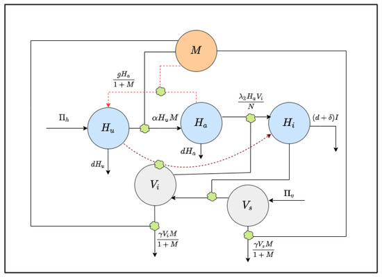
Figure 1.
Schematic diagram of the model (1): interactions between model populations are shown.
Let be the constant growth of the human population, either by birth or immigration. The whole human population experiences a natural mortality . Unaware people become aware due to the awareness campaign through social media at a rate . It is assumed that being aware, people will take all necessary precautions, such as use mosquito nets and spray insecticides, for personal defense from the disease. Thus, the infection rate decreases with the increase in the level of awareness. Aware people may be unaware at a rate g, but the rate decreases with the level of awareness [24]. The model captures this fact with the term .
Let be the constant growth rate of the susceptible mosquito population. The rate of infections for susceptible humans is and that of susceptible vectors is .
In the modeling development, it is assumed that the media campaigns increase the level of awareness regarding self-protection and the methods for reducing the mosquito population [22]. Here, the level of awareness among people rises at a constant rate due to the campaign through global sources, such as radio and TV. It also increases through local campaigns and is proportional to the number of infected cases at a rate ; it declines at a rate due to fading of memory [25].
Moreover, the constants r and , respectively, signify the recovery rate and disease-induced death rate of the population. The recovery of infected humans relies on the awareness campaign. For the mosquito population, denotes the natural death rate.
Knowing the disease and control measures through the awareness movements, people will use insecticides to eliminate mosquitoes at a rate , modeled via the term and , where is the maximum rate of insecticide usage.
With the above assumptions, the following mathematical model is derived:
Subjected to the initial conditions
3. Basic Properties of the Model
In this section, the basic properties of system (1), such as non-negativity and boundedness of solutions, are discussed. In addition, the basic reproduction number is determined for analysing the dynamics of system (1).
3.1. Non-Negativity and Boundedness of the Solutions
The for the effect of awareness on the transmission dynamics of malaria will be analyzed in a biologically and mathematically viable region as follows. This region should be feasible for habitation by both the human and mosquito populations. Hereafter, the following proposition is established.
Proof.
Let
Since , and , then . If , then are all equal to zero at .
It follows from the first equation of system (1) that
That is,
Thus,
Hence,
So that,
From the second equation of system (1), we can write
That is
Thus,
Hence,
So that
Following the same procedure, it can be shown that , and for all . □
Proposition 2.
Every solution of system (1) is uniformly bounded in the region
Proof.
At any time t, . Then, the derivative of with respect to time t, along the solution of system (1) is determined as
Then, from the above, we have
So that
That means
Similarly, for any time t, if we let , then the derivative of with respect to t along the solution of system (1) is obtained as
Thus, the above calculation gives
So that
Thus, we finally have
Finally, from the last equation of system (1), one can obtain
On solving this linear differential inequality, we obtain
So that
Hence,
From (4)–(6), we can conclude that the set is positively invariant. Therefore, it is adequate to contemplate the dynamics of system (1) in . In this region, the model is biologically and mathematically well-posed. Moreover, each solution of the model (1) with initial condition (2) that starts in remains in for all . □
3.2. The Basic Reproduction Number
The basic reproduction number, generally denoted by , is often considered as the threshold quantity that determines the dynamic behavior of the model [26].
The method as used by Heffernan et al. in [27] has been followed for determining the basic reproduction number .
Here, the next generation matrix is denoted by . It comprises two matrices, namely F and V, where
The reproduction number is obtained as . Here, is the dominant eigenvalue of the matrix .
Hence,
where, .
4. Existence of Equilibrium Points
The model system (1) has two equilibrium points, namely the disease-free equilibrium, (DFE), and the endemic equilibrium point (EEP), .
4.1. The Disease-Free Equilibrium (DFE)
The system (1) has a disease-free equilibrium , where
4.2. The Endemic Equilibrium Point (EEP)
The endemic equilibrium point of the malaria model (1) is represented as , where
where and is the positive root of
Remark 1.
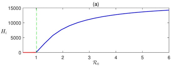
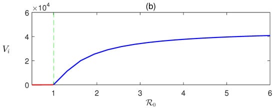
Here, we derive that in terms of and can be determined numerically using (8). Detailed numerical calculations show that EEP exists when , that is when DFE is unstable (Figure 2).
Figure 2.
Forward transcritical bifurcation: equilibrium values of (a) infected human and (b) infective vectors are plotted with respect to the basic reproduction number . The parameter is varied, and the rest of the parameters’ values are taken from Table 1.
5. Jacobian Matrix and Stability Analysis of Equilibrium Points
The Jacobian matrix at any steady point is given by
where the elements of the matrix are given below:
5.1. Local Stability Analysis of Disease-Free Equilibrium (DFE)
The following theorem analyses the local stability of DFE.
Theorem 1.
The DFE of the model Equation (1), given by , is locally asymptotically stable (LAS) if and unstable if .
Proof.
Using (9), we calculate the Jacobian matrix at the disease-free equilibrium point as,
The characteristic equation of in x is
Two eigenvalues, and , are negative. Since , , and are positive, according to Routh–Hurwitz criteria, the rest of the eigenvalues are negative only if , that is if .
This implies .
This gives
Therefore, the disease-free equilibrium of the malaria model (1) is locally asymptotically stable when . □
Remark 2.
From an epidemological point of view, malaria can be eliminated from the community when . If , then on average an infected individual produces less than one new infected individual over its infectious period, and the infection dies out. However, if , then each infected individual produces on average more than one infection, and the disease persists and invades the population. We verified the results for our systems using numerical simulations (see Figure 2).
5.2. Global Stability of DFE
This subsection investigates the global asymptotic stability of the disease-free equilibrium (DFE) following the method proposed in [29].
The system (1) can be rewritten as
where is the uninfected, and is the infected population. In addition, denotes the DFE of system (11). If the DFE satisfies the following two conditions,
- (i)
- For , is globally asymptotically stable,
- (ii)
- ,
then is globally asymptotically stable [29].
Using the above result, we derive the following theorem for system (1).
Theorem 2.
For , the DFE of system (1) is globally asymptotically stable if: (a) the conditions (i) and (ii) are satisfied, and (b) .
Proof.
We introduce two new variables and to divide the system into two subsystems. From Equation (1), we have two vector-valued functions, and , given by
and
The reduced system corresponding to condition (i) is obtained as
We note that this asymptomatic dynamic is independent of the initial conditions in ; therefore, the convergence of the solutions of the reduced system (12) is global in . We compute
and show that Now,
Thus, we obtain
Here, . Thus, for all . In addition, since all off-diagonal elements of the matrix A are non-negative, A is an M-matrix. Therefore, this proves that the DFE is globally asymptotically stable (GAS). □
5.3. Local Stability of EEP
Using the Jacobian matrix in (9), a characteristic equation in can be obtained from the following relation,
where I is a identity matrix.
The characteristic equation at is derived from (13) as,
The coefficients of (14) are given in Appendix A.
According to Routh–Hurwitz conditions, the characteristic Equation (14) has roots with negative real parts if the following conditions are satisfied:
6. The Optimal Control Problem
In this section, the system (1) is reformulated by incorporating three time dependent control functions, , and . The first control function is taken for controlling the cost of treatment, the second control for controlling the cost of insecticides, and the third control is for control of the cost of arranging awareness campaigns.
The system (1) is reformulated incorporating the control parameters as follows,
with the initial conditions
The objective function for the minimization problem is proposed as
where the quantities , , and are positive constants representing the weight constants on the benefit of the cost, whereas the quantities and are the penalty multipliers. In the optimal control problem, we assume that the value is fixed.
For the optimal control problem, we have assumed a quadratic objective functional because the cost takes a nonlinear form, and it also prevents the bang-bang or singular optimal control cases [30].
The intention here is to find the optimal profiles of the control functions , and , denoted, respectively, as so that is minimum. That means
subject to the state system (16), where
is an admissible control set.
6.1. Existence of the Optimal Control Triple
Theorem 3.
Given the objective functional
subject to system (16) with their initial conditions. Then, there exists an optimal control triple and corresponding state solution such that if the following five conditions are satisfied,
- (i)
- (ii)
- The control set is convex and closed;
- (iii)
- Each right-hand side of the state system (16) is: (a) continuous, (b) bounded above by a sum of the bounded control and the state variables, and (c) can be written as a linear function of u with time and the state-dependent coefficients;
- (iv)
- The integrand function of the objective functional is convex on ;
- (v)
- There exist positive numbers and a constant such that
Proof.
A detailed proof of this theorem can be obtained from [31,32] or [30]. □
6.2. Characterization of the Optimal Control
The objective function denotes the total cost. It is achieved as a result of the application of control measures and the burden of the disease. The following theorem characterizes the optimal control.
Theorem 4.
Given the optimal controls and the solutions of the corresponding state system (16), then there exist adjoint variables satisfying the following system of equations
with transversality conditions
Moreover, the optimal controls, , and , for are given by
Proof.
Let be optimal controls whose existence is assured by Theorem 3. The Pontryagin minimum principle (PMP) [33] provides necessary optimality conditions that must satisfy. For the optimal control problem, we take the Hamiltonian as
where are the adjoint variables or co-state variables.
The PMP converts the optimal control problem to a static optimization problem that is a problem of minimizing the Hamiltonian in the control space.
From the above analytical analysis, we obtain the optimality system which consists of the state system (16) with the initial conditions (17), the adjoint system (20) with the boundary conditions (21), and the optimal controls (10) as follows:
Remark 3.
The optimality system is a two-point boundary value problem. The state system (16) is an initial value problem with initial condition (17), and the adjoint system (20) is a boundary value problem with boundary condition . The optimality system has a unique solution for some small time in light of the fact that the solutions of the state and adjoint system are bounded and satisfy Lipschitz conditions. Thus, a restriction on the length of the time interval in the control problem ensures the uniqueness of the optimality system.
7. Numerical Simulations
In this section, numerical results are achieved on the basis of analytical calculations. The values of the parameters used in numerical simulations are listed in Table 1.

Table 1.
Biological meanings of variables, parameters used in the model (1), and values of the parameters used for numerical simulations [22,28].
In Figure 2, the forward bifurcation of is sketched. For , the disease-free equilibrium is stable and unstable otherwise. Consequently, transcritical bifurcation has occurred at . This shows the existence of a unique endemic equilibrium .
In Figure 3a–f, the numerical solution of the proposed model system is plotted with two different values of awareness rates. This figure confirms that the influence of consciousness over media has an important role in monitoring malaria transmission. The endemic equilibrium point is obtained as , and it is asymptotically stable. Figure 4 shows that the endemic equilibrium point , when it exists, is nonlinearly stable, i.e., all the phase portraits converge to the same endemic equilibrium for different initial values.
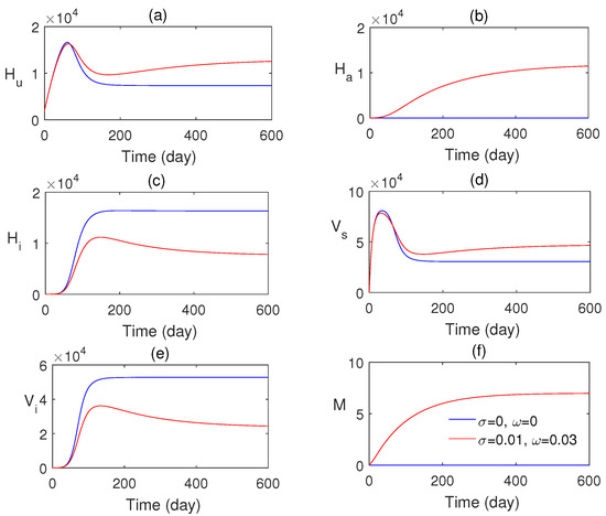
Figure 3.
Numerical solution of system (1) with and without the impact of awareness.
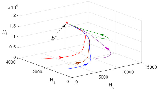
Figure 4.
Phase portrait is plotted in phase space. Parameter values are the same as in Figure 3.
In Figure 5a–f, the equilibrium values of the infected human population are plotted concerning local awareness rate . The infection rate decreased significantly due to the effect of the local awareness campaign. So, local health centers should organize consciousness movements about the disease. We also plotted the steady state values of the infected human population with respect to global awareness . A rapid decrease in the infected population is observed in Figure 6a–f. Hence, through global media (radio, TV, etc.), awareness about the disease is raised.
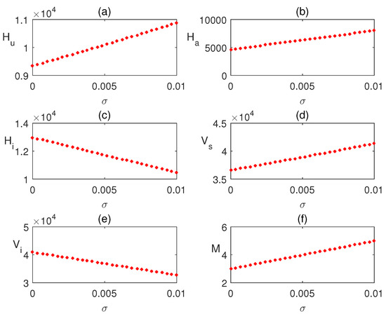
Figure 5.
Effect of local awareness is shown varying the parameter .
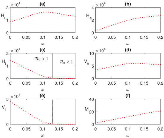
Figure 6.
Effect of global awareness is shown varying the parameter . Other parameters values are as shown in Figure 3.
Figure 7 shows the instantaneous effect of the local and global responsiveness movement on the infected human population in space. Infections decreased due to the impact of both consciousness movements.
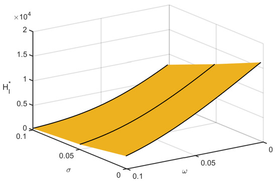
Figure 7.
Combined effects of local and global awareness on infected population.
7.1. Numerical Solution of the Optimal Control Problem
Here, results from the numerical simulations of the optimality system (24) are presented with the help of MATLAB.
The optimal control problem deals with the control’s effect on the development of malaria and also entails the cost sustained in their implementation. The optimal solution is obtained by solving the optimality system numerically which contains six ordinary differential equations (ODEs) for both the state and adjoint equations.
The state system is an initial value problem, whereas the adjoint system is a boundary value problem. We used an iterative scheme (using the fourth-order Runge–Kutta scheme) for solving the state system with an initial guess for the control functions over the desired time. In addition, the adjoint equations are solved backward in time using the current iteration of the state equations. In the iterative scheme, the values of the control functions are updated by using a convex combination of the preceding control functions and the values from the characterization. This process is continued until the difference between the values of the unknowns in the earlier iteration and in the current iteration is negligible [34].
Numerical simulations of the optimal control problem are plotted in Figure 8 and Figure 9. Figure 8a–d compares the system with and without optimal control. It is found that optimal control has a substantial advantage in monitoring the system. The corresponding optimal profiles of the control variables are plotted in Figure 9a–c. The optimal profiles of the controlling agents indicate that more insecticide spraying is essential.
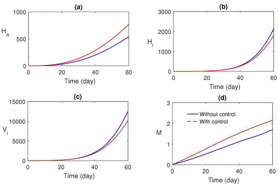
Figure 8.
Comparison between the system with and without optimal control.
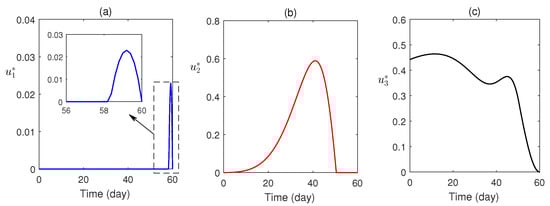
Figure 9.
The profiles of optimal controls are plotted as a function of time.
8. Discussion
This article uses a mathematical model to analyze media campaigns’ influence on malaria dynamics. To our knowledge, few articles are available on this topic. Before discussing the main results, a comparison between the proposed model and the existing mathematical models is made.
Al Basir et al., 2020 [22] proposed a mathematical model (using delay differential equations) using human (susceptible and infected) and mosquito populations (susceptible and infected). They assumed the `level of awareness’ as a separate population for the impact of social media campaigns. Rather than applying optimal control theory, they focused on the effect of delay in organizing the campaign. In contrast, in our research, media awareness is assumed as a separate model population that changes with time. In addition, susceptible humans are divided into aware and unaware human classes. Moreover, optimal control theory was applied to maximize the awareness level and cost-effectiveness.
In [23], the authors divided infected humans into aware and unaware infected human populations. In addition, the study assumed media as separate model variables whose growth is assumed proportional to the unaware infected human population. They did not divide the susceptible humans into aware and unaware classifications. In contrast, our research divides susceptible humans into aware and unaware classes, which is more realistic [21]. Moreover, the infected humans recover through awareness-induced treatment, and after recovery, they join the aware human population. This hypothesis is more realistic.
In [13], the authors formulated a mathematical model using human (susceptible, infected, recovered) and mosquito (susceptible and infected) populations. The susceptible population was divided into aware and unaware susceptible humans. Finally, they applied optimal control for cost minimization and optimal control of the disease. They did not assume that recovered people again become susceptible and aware of the disease. In addition, the effect of awareness was modeled using constant terms.
In our research, it is additionally assumed that infected humans recovered with awareness-induced treatment, and after recovery, they join the aware human population, which is more realistic than other models. In the proposed model, ‘level of awareness’ is taken as a model variable, increasing due to awareness campaigns (as adopted by Al Basir et al. [22]). The local awareness (due to the information from local people and relatives) and global awareness (due to radio and TV campaigns) are also included in the model. We further assumed that the aware people become unaware but those numbers decrease with the level of awareness, . Aware people may become infected at a much lower rate than unaware humans. Optimal control theory was applied to maximize awareness and minimize the disease control cost.
Thus, the awareness-based model proposed here is more functional and can capture the dynamics of malaria with awareness-based interventions. In addition, the control-induced model can minimize the cost of malaria management.
The dynamics of malaria propagation were studied using the proposed mathematical models analytically and numerically. Using the next-generation matrix, the basic reproduction number was derived. Equilibria assessment showed two equilibria of the proposed model: the disease-free and endemic. The disease-free equilibrium is stable for and the endemic equilibrium exists for , that is, when the disease-free equilibrium becomes unstable. The endemic equilibrium, when it exists, is globally asymptotically stable.
Optimal control theory was applied to awareness-induced interventions for the cost-effective treatment of malaria. The proposed optimal system was analytically solved using the Pontryagin minimum principle (Section 6) and numerically solved (using the scheme stated in Section 7.1). The optimal profiles of the control variables (Figure 9) were plotted. It was established that the optimally controlled system is essential and effective in malaria control (Figure 8).
9. Conclusions
Malaria, one of the world’s most significant diseases, is a mosquito-borne human disease caused by a parasite transmitted by the female Anopheles mosquito. Mathematical modeling and control theory help in predicting the dynamics of the disease and are also helpful for practical policy making. Awareness campaigns about the disease are also equally important in controlling the disease.
In this article, a mathematical model was proposed for a malaria dynamic, considering the impact of awareness-based control approaches. The dynamics of the system were analyzed using qualitative stability theory. The optimal control concept was applied for cost minimization in disease control. Pontryagin’s minimum principle was implemented for the optimization of the system.
The control-induced model helps optimal disease control with minimum advertising, insecticide, and treatment costs using the minimum principle. The obtained results are helpful for policy makers in proposing suitable control strategies against malaria. In a nutshell, the awareness movement is vital for controlling malaria, and applying optimal control theory along with media consciousness is required.
Author Contributions
Conceptualization, F.A.B.; Methodology, T.A.; Formal analysis, T.A.; Investigation, F.A.B.; Writing—original draft, F.A.B. All authors contributed equally to each part of this work. All authors have read and agreed to the published version of the manuscript.
Funding
This research received no external funding.
Data Availability Statement
The data that support the findings of this study are available from the corresponding author upon reasonable request.
Conflicts of Interest
The authors declare no conflict of interest.
Appendix A
References
- World Health Organisation. Malaria. 2021. Available online: https://www.who.int/news-room/fact-sheets/detail/malaria (accessed on 28 April 2021).
- Dyer, O. African Malaria Deaths Set to Dwarf COVID-19 Fatalities as Pandemic Hits Control Efforts, WHO Warns; WHO: Geneva, Switzerland, 2020. [Google Scholar]
- World Health Organization. The Potential Impact of Health Service Disruptions on the Burden of Malaria: A Modelling Analysis for Countries in Sub-Saharan Africa; WHO: Geneva, Switzerland, 2020. [Google Scholar]
- Bakare, E.A.; Nwozo, C.R. Mathematical analysis of the dynamics of malaria disease transmission model. Int. J. Pure Appl. Math. 2015, 99, 411–437. [Google Scholar] [CrossRef][Green Version]
- Adongo, P.B.; Kirkwood, B.; Kendall, C. How local community knowledge about malaria affects insecticide-treated net use in northern Ghana. Trop. Med. Int. Health 2005, 10, 366–378. [Google Scholar] [CrossRef] [PubMed]
- Briscoe, C.; Aboud, F. Behaviour change communication targeting four health behaviours in developing countries: A review of change techniques. Soc. Sci. Med. 2012, 75, 612–621. [Google Scholar] [CrossRef] [PubMed]
- Ankomah, A.; Adebayo, S.B.; Arogundade, E.D.; Anyanti, J.; Nwokolo, E.; Inyang, U.; Ipadeola, O.B.; Meremiku, M. The Effect of Mass Media Campaign on the Use of Insecticide-Treated Bed Nets among Pregnant Women in Nigeria. Malar. Res. Treat. 2014, 2014, 694863. [Google Scholar] [CrossRef] [PubMed]
- Dhawan, G.; Joseph, N.; Pekow, P.S.; Rogers, C.A.; Poudel, K.C.; Bulzacchelli, M.T. Malaria-related knowledge and prevention practices in four neighbourhoods in and around Mumbai, India: A cross-sectional study. Malar. J. 2014, 13, 303. [Google Scholar] [CrossRef][Green Version]
- Okosun, K.O.; Rachid, O.; Marcus, N. Optimal control strategies and cost-effectiveness analysis of a malaria model. BioSystems 2013, 111, 83–101. [Google Scholar] [CrossRef]
- Abioye, A.I.; Ibrahim, M.O.; Peter, O.J.; Ogunseye, H.A. Optimal control on a mathematical model of malaria. Sci. Bull. Ser. A Appl. Math Phys. 2020, 82, 178–190. [Google Scholar]
- Romero-Leiton, J.P.; Ibargüen-Mondragón, E. Stability analysis and optimal control intervention strategies of a malaria mathematical model. Appl. Sci. 2019, 21, 184–218. [Google Scholar]
- Misra, A.K.; Pal, S.; Gupta, R.K. Modeling the Effect of TV and Social Media Advertisements on the Dynamics of Vector-Borne Disease Malaria. Int. J. Bifurc. Chaos 2023, 33, 2350033. [Google Scholar] [CrossRef]
- Ndii, M.Z.; Adi, Y.A. Understanding the effects of individual awareness and vector controls on malaria transmission dynamics using multiple optimal control. Chaos Solitons Fractals 2021, 153, 111476. [Google Scholar] [CrossRef]
- Nwankwo, A.; Okuonghae, D. A mathematical model for the population dynamics of malaria with a temperature dependent control. Differ. Equ. Dyn. Syst. 2022, 30, 719–748. [Google Scholar] [CrossRef]
- Noeiaghdam, S.; Micula, S. Dynamical Strategy to Control the Accuracy of the Nonlinear Bio-mathematical Model of Malaria Infection. Mathematics 2021, 9, 1031. [Google Scholar] [CrossRef]
- Kobe, F.T. Mathematical Model of Controlling the Spread of Malaria Disease Using Intervention Strategies. Pure Appl. Math. J. 2020, 9, 101. [Google Scholar] [CrossRef]
- Handari, B.D.; Vitra, F.; Ahya, R.; Nadya, S.T.; Aldila, D. Optimal control in a malaria model: Intervention of fumigation and bed nets. Adv. Differ. Equ. 2019, 2019, 497. [Google Scholar] [CrossRef]
- Nájera, J.A.; González-Silva, M.; Alonso, P.L. Some lessons for the future from the Global Malaria Eradication Programme (1955–1969). PLoS Med. 2011, 8, e1000412. [Google Scholar] [CrossRef]
- Karunamoorthi, K. Vector control: A cornerstone in the malaria elimination campAign. Clin. Microbiol. Infect. 2011, 17, 1608–1616. [Google Scholar] [CrossRef]
- Mazigo, H.D.; Obasy, E.; Mauka, W.; Manyiri, P.; Zinga, M.; Kweka, E.J.; Heukelbach, J. Knowledge, attitudes, and practices about malaria and its control in rural northwest Tanzania. Malar. Res. Treat. 2010, 2010, 794261. [Google Scholar] [CrossRef]
- Misra, A.K.; Sharma, A.; Li, J. A mathematical model for control of vector borne diseases through media campaigns. Discret. Contin. Dyn. Syst. 2013, 18, 1909. [Google Scholar] [CrossRef]
- Al Basir, F.; Banerjee, A.; Ray, S. Exploring the effects of awareness and time delay in controlling malaria disease propagation. Int. J. Nonlinear Sci. Numer. Simul. 2021, 22, 665–683. [Google Scholar] [CrossRef]
- Ibrahim, M.M.; Kamran, M.A.; Naeem Mannan, M.M.; Kim, S.; Jung, I.H. Impact of awareness to control malaria disease: A mathematical modeling approach. Complexity 2020, 2020, 1–13. [Google Scholar] [CrossRef]
- Al Basir, F.; Ray, S.; Venturino, E. Role of media coverage and delay in controlling infectious diseases: A mathematical model. Appl. Math. Comput. 2018, 337, 372–385. [Google Scholar] [CrossRef]
- Agaba, G.O.; Kyrychko, Y.N.; Blyuss, K.B. Dynamics of vaccination in a time-delayed epidemic model with awareness. Math. Biosci. 2017, 294, 92–99. [Google Scholar] [CrossRef] [PubMed][Green Version]
- Smith, D.L.; McKenzie, F.E.; Snow, R.W.; Hay, S.I. Revisiting the basic reproductive number for malaria and its implications for malaria control. PLoS Biol. 2007, 5, e42. [Google Scholar] [CrossRef] [PubMed]
- Heffernan, J.M.; Smith, R.J.; Wahl, L.M. Perspectives on the basic reproductive ratio. J. R. Soc. Interface 2005, 2, 281–293. [Google Scholar] [CrossRef]
- Lashari, A.A.; Aly, S.; Hattaf, K.; Zaman, G.; Jung, I.H.; Li, X.-Z. Presentation of malaria epidemics using multiple optimal controls. J. Appl. Math. 2012, 2012, 946504. [Google Scholar] [CrossRef]
- Castillo-Chavez, C.; Blower, S.; Driessche, P.; Kirschner, D.; Yakubu, A. Mathematical Approaches for Emerging and Reemerging Infectious Diseases: Models, Methods, and Theory; Springer: Berlin/Heidelberg, Germany, 2002. [Google Scholar]
- Fleming, W.H.; Rishel, R.W. Deterministic and Stochastic Optimal Control; Springer: Berlin/Heidelberg, Germany, 1975. [Google Scholar]
- Roy, P.K.; Roy, A.K.; Khailov, E.N.; Basir, F.A.; Grigorieva, E.V. A model of the optimal immunotherapy of psoriasis by introducing IL-10 AND IL-22 inhibitors. J. Biol. Syst. 2020, 28, 609–639. [Google Scholar] [CrossRef]
- Abraha, T.; Basir, F.A.; Obsu, L.L.; Torres, D.F. Farming awareness based optimum interventions for crop pest control. Math. Biosci. Eng. 2021, 18, 5364–5391. [Google Scholar] [CrossRef]
- Fleming, W.; Lions, P.-L. Stochastic Differential Systems, Stochastic Control Theory and Applications: Proceedings of a Workshop, Held at IMA, 9–19 June 1986; Springer Science & Business Media: Berlin/Heidelberg, Germany, 1986; Volume 10. [Google Scholar]
- Lenhart, S.; Workman, J.T. Optimal Control Applied to Biological Models; Chapman & Hall/CRC: Boca Raton, FL, USA, 2007. [Google Scholar]


Disclaimer/Publisher’s Note: The statements, opinions and data contained in all publications are solely those of the individual author(s) and contributor(s) and not of MDPI and/or the editor(s). MDPI and/or the editor(s) disclaim responsibility for any injury to people or property resulting from any ideas, methods, instructions or products referred to in the content. |
© 2023 by the authors. Licensee MDPI, Basel, Switzerland. This article is an open access article distributed under the terms and conditions of the Creative Commons Attribution (CC BY) license (https://creativecommons.org/licenses/by/4.0/).