Abstract
This study presents numerical work to investigate the Falkner–Skan flow of a bio-convective Casson fluid over a wedge using an Evolutionary Padé Approximation (EPA) scheme. The governing partial differential equations and boundary conditions of a Falkner–Skan flow model are transformed to a system of ordinary differential equations involving ten dimensionless parameters by using similarity transformations. In the proposed EPA framework, an equivalent constrained optimization problem is formed. The solution of the resulting optimization problem is analogous to the solution of the dimensionless system of ordinary differential equations. The solutions produced in this work, with respect to various combinations of the physical parameters, are found to be in good agreement with those reported in the previously published literature. The effects of a non-dimensional physical-parameter wedge, Casson fluid, fluid phase effective heat capacity, Brownian motion, thermophoresis, radiation, and magnetic field on velocity profile, temperature profile, fluid concentration profile, and the density of motile microorganisms are discussed and presented graphically. It is observed that the fluid velocity rises with a rise in the Casson fluid viscosity force parameter, and an increase in the Prandtl number causes a decrease in the heat transfer rate. Another significant observation is that the temperature and fluid concentration fields are greatly increased by an increase in the thermophoresis parameter. An increase in the Péclet number suppresses the microorganism density. Moreover, the increased values of the Prandtl number increase the local Nusslet number, whereas the skin friction is increased when an increase in the Prandtl number occurs.
MSC:
76A05; 80A19; 35Q30
1. Introduction
Researchers have been investigating for decades to find new strategies to manage the greenhouse effect. The primary goal is to discover new more effective techniques for controlling environmental conditions. Microorganisms absorb carbon dioxide more effectively than plants. Bio-convection is an unstructured pattern in the state of suspension produced by microorganisms, which are denser than ordinary creatures moving upwards in water. Because of the concentration of self-propelled microbes, the upper layer of fluid becomes extremely dense and thus unstable. Therefore, additional upward swimming of these motile microorganisms causes a crumbling of microorganisms, resulting in the creation of bio-convection. Bio-convection has many uses, including mass transit phenomena, bio-reactors, biodiesel fuels, winemaking, fuel cell technologies, and food processing. The historical traces reveal that Harris [1] and Bird et al. [2] made substantial contributions to the research on numerous rheological aspects of non-Newtonian fluid flow models. The role of Brownian motion, first explained by Batchelor [3], in maintaining small particles suspended in rheological processes has been found vital. In an infinite fluid, the dilution of the disruption of rigid spherical particles via isotropic structure suspension and hydrodynamic processes is classically justified as a function of the physical parameters involved in rheological flow. Later, Hillesdon et al. [4] and Guell et al. [5] initiated research on bio-convection flows, discovering their usefulness in the aforementioned applications. There is no evidence of impacts of Brownian motion of diffusion particles in a boundary layer momentum.
A notable aspect is that the pressure or stress force applied in fluid flow results in strong hydrodynamic interactions. Alloui et al. [6] utilized the Navier–Stokes model to investigate the arrangement of microorganisms in a cylinder. Ishikawa and Pedley [7] presented a model of microorganism swimming behavior as a squirming sphere that ignored the effects of Brownian motion and microorganism inertia. Mehandia and Nott [8] investigated the collective dynamics of self-propelled particles, Pedley [9] revisited the instability of uniform microorganism suspensions, Nguyen-quang and Guichard [10] investigated the role of bio-convection in plankton populations with thermal stratification, and Ghorai, Panda, and Hill [11] presented bio-convection in a suspension of isotropically scattering phototactic algae. Kuznetsov [12] introduced the computational model of nanofluid bio-convection in porous media for the first time. He discovered that cell deposition influences the evolution of bio-convection. Because of its importance in industry, chemical engineering, and biological processes, there has been a significantly strong research trend in non-Newtonian transport and flow processes in fluids in recent years.
Making optical fibers, clay coatings, cosmetic items, and plastic polymers are several examples of such applications. In the presence of numerous varieties of non-Newtonian fluids, it is impossible to model significant rheological characteristics of their flows perfectly through a single natural law connecting shear rate and shear stress. As extensions of these studies, several researchers [13,14,15,16,17] have investigated the characteristics of non-Newtonian flow constrained to various flow-regulating parameters. In the light of practical applications of magnetohydrodynamic flow of an electrically conducting fluid over a heated surface in areas such as plasma studies, the petroleum industry, cooling of nuclear reactors, the boundary layer resistor in aerodynamics, magnetohydrodynamic power generators, and crystal growth, its study has drawn the attention of several researchers. Similarly, the forced, steady-state, and mixed-type convections on the magnetohydrodynamic flow also ignite substantial theoretical and practical interests when they occur in combination with various characteristics of surface geometries and boundary flow. Mukhopadhyay et al. [18] examined boundary-layer forced convection flow of a Casson fluid past a symmetric wedge, and Animasaun et al. [19] studied the impacts of thermal radiation and magnetic field on unbalanced diffusivities of homogeneous and heterogeneous reactions in viscoelastic fluid flow. The unsteady three-dimensional flow of Casson–Carreau fluids past a stretching surface was studied by Raju and Sandeep [20]. The impact of Stefan blowing on bio-convection past a stretchable sheet was introduced by Uddin et al. [21], whereas Dhanai et al. [22] identified the existence of dual and stable solutions to the hydromagnetic bio-convection slip model over a sheet with non-zero inclination. Coelho et al. [23] investigated two scenarios of laminar-forced convection in pipes and channels using the Phan-Thien-Tanner (SPTT) model, assuming fully developed conditions. Francisca et al. [24] explored heat transfer in a channel of Couette–Poiseuille flow under the impact of viscous dissipation for stable, laminar flow, and both hydro-dynamically and thermally completely developed a pseudo-plastic fluid. In 2017, Chamkha et al. [25] proposed a nanofluid with gyrotactic microorganisms possessing bio-convective flow freely over a vertical radiating plate. Recently, Rashad et al. [26,27] have investigated the mixed bio-convection flow of similar nanofluids past a vertical trim cylinder. Several theoretical models exist for analyzing the flows over the wedge in the presence of magnetic fields, chemical reactions, and sink and heat source parameters. But the involvement of gyrotactic microorganisms makes it challenging to study Brownian motion and thermophoresis effects on magnetohydrodynamic flow over a wedge. To overcome such complexities, Raju and Sandeep [28] studied a Falkner–Skan type model [29] of Brownian motion and thermophoresis effects on Casson fluid flow past a wedge.
Solving Falkner–Skan-flow-type bio-convection problems with Brownian motion is a challenging task when opting for classical finite difference or analytical methods. Falkner–Skan flow models are complex due to high nonlinearity, asymptotic boundary conditions, and the involvement of several fluid parameters. Finite difference schemes [30] are better suited for initial value problems. The complex geometries involved in Falkner–Skan bio-convection models make these methods less reliable, as they not only depend on discretization step size but also lack the mechanism for handling asymptotic conditions. Spectral methods [31,32] and semi-analytical techniques for integer-order models [33,34] and fractional models [35,36,37] are better only in small domains. On the other hand, solving differential equations by transforming them into equivalent optimization problems is one of the modern approaches. These techniques are based on smart fusions of mathematics and artificial intelligence. Early instances of such implementations include solutions of nonlinear ordinary differential equations by swarm intelligence [38] and genetic algorithms [39,40]. The solution of partial differential equations by an evolutionary algorithm was proposed by Panagant and Bureerat [41].
This work analyzes heat and mass transfer in the Falkner–Skan flow of a bio-convective Casson fluid by an evolutionary Padé approximation (EPA) scheme proposed by Ali et al. [42]. The EPA scheme is a new soft computing scheme that was initially used to obtain closed-form approximate solutions of coupled dynamical systems while preserving vital properties of the dynamical models in computer networks [42] and COVID-19 disease predictions [43]. Later, Nisar et al. [44] successfully applied the EPA scheme to solve nonlinear PDEs.
The strength of the EPA scheme in solving complex problems lies in the interpolating and extrapolating properties of Padé rational functions and modern artificial intelligence-assisted algorithms. Contrary to conventional techniques, the EPA method does not depend on discretization step sizes. The EPA scheme directly embeds asymptotic boundary conditions into the solutions and transforms unknown initial conditions into decision variables that are determined by an optimizer while satisfying the model equations. On the other hand, classical schemes rely on initial guesses and a hit-and-miss approach because they neither inherit mechanisms to determine the unknown initial conditions nor handle the infinity boundary conditions. Another benefit of the EPA approach over other semi-analytical methods is that the problem domain is not required to be transformed into smaller domains. These arguments highlight that conventional methods require more computational efforts to obtain good approximates of exact solutions and, hence, the EPA scheme offers an effective alternative choice that optimally generates acceptable solutions using a self-trained computational framework. The main contributions of this work are stated below.
- (i)
- This study presents the analysis of heat and mass transfer in the Falkner–Skan flow of a bio-convective Casson fluid past a wedge by an artificial-intelligence-based paradigm. To the best of the authors’ knowledge, this is the first application of the EPA scheme to analyze the Falkner–Skan flow of bio-convective Casson fluid over a wedge.
- (ii)
- This work introduces the usage of Padé rational functions to handle asymptotic boundary conditions. This aspect is an interesting new direction in hybridizing convention-based semi-analytic methods to obtain a rationally tailed approximate solution to the model.
- (iii)
- As far as the authors’ intentions are concerned, the current script can be viewed as the first step towards the development of an artificial intelligence-assisted code for analyzing heat and mass transfer in fluid dynamics.
2. Problem Statement
A two-dimensional Falkner–Skan model of steady magneto-hydrodynamic (MHD) Casson fluid flow (CFF) past a wedge packed by gyrotactic microorganisms has been considered for analysis. It is assumed that Brownian motion and the thermophoresis effect both exist. The total wedge angle, is non-zero, where . The parameter relates to the Falkner–Skan power law. Physically, the negative value of the parameter corresponds to an opposing pressure gradient caused by boundary layer split-up, whereas the positive value relates to an additional pressure gradient. The zero value indicates that the flow is not in the Falkner–Skan sense.
Another assumption is that the flow direction is constrained by the changing magnetic field, as denoted by . The isotropic CFF is described by the following rheological model [17,28]:
Here, , , being the element of deformation rate. and denote the critical value of and dynamic viscosity, respectively, based on the non-Newtonian fluid. is used to denote the fluid’s yield stress.
Let us denote velocity components along and axes by and , respectively, temperature by , concentration of the fluid molecules by , and density of moving microorganisms by . The velocity, temperature, fluid concentration at the wedge are denoted as , , and , respectively, whereas the velocities, temperature, and concentration at free stream are , , and , respectively. It is assumed that the decomposition between fluid particles and microorganisms is uniform. The Boungrino nanofluid model has been used to observe the thermophoretic and Brownian motion features. Under these assumptions regarding isotropic CFF and the dynamical behavior of the Falkner–Skan model exhibited in Figure 1, the boundary layer governing system of partial differential equations with respect to the stream function , with and , can be written as [13,19,22]:
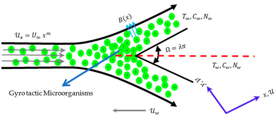
Figure 1.
Physical configuration of Falkner–Skan flow model.
Subject to the boundary conditions:
In systems (1) and (2) all subscripts involving and denote the partial derivatives whereas all other subscripted symbols denote constants. In system (1) the first equation is continuity equation, the second equation is related to velocity, the third equation models the heat transfer, the fourth equation is related to concentration, and the fifth and final equation presents density of motile microorganisms. If then the fluid is Newtonian otherwise it is non-Newtonian. The parameters , , , and denote the maximum swimming speed of the cell, kinematic viscosity, density, and conductivity of the fluid, respectively. Gravitational acceleration is denoted by , the capacitance is abbreviated as , denotes the coefficient of thermophoretic diffusion, represents density of coefficient of diffusion, dynamic viscosity is denoted by , represents the aggregate absorption coefficient, is the chemo taxis coefficient, and is the Stefan-Boltzmann coefficient.
In order to convert system (2) to an equivalent system of ordinary equations, we use dimensionless variable in following similarity transformation functions.
The transformations (3) automatically satisfy the first continuity equation of system (1). Remaining equations of system (1) are transformed to a system of coupled nonlinear differential Equations (4)–(7), and boundary conditions (2) are converted to new boundary conditions (8).
The transformed boundary conditions are as follows:
In above transformed system, the flow is in the Falkner–Skan sense if . The parameters , , and denote the Péclet, Prandtl, and Lewis numbers, respectively. The parameters , , , , , and are related to Brownian motion, thermophoresis, radiation, fluid parameter, magnetic field, and the wedge, respectively. The effective heat capacity of the fluid phase with respect to the particle is denoted by . These dimensionless parameters are defined as follows:
The essential physical quantities are defined as follows:
3. Evolutionary Padé Approximation (EPA) Framework
This section presents the framework of EPA technique for solving the Falkner–Skan flow of a bio-convective Casson fluid. Firstly, coupled system defined by Equations (4)–(7) is transformed to an unconstrained optimization problem by approximating , , , and by Padé functions. Secondly, for solution of the resulting optimization problem, we present a hybrid algorithm based on an evolutionary optimizer, called differential evolution (DE) [45], and a local search algorithm, called Nelder-Mead simplex (NMS) method [46].
3.1. Formulation of Equivalent Optimization Problem
Padé rational function with order are used to approximate , , , and , respectively, for . The Padé rational function is given as [38,39]:
Provided that and are polynomial functions given as:
Expressing the first, second, and third order derivatives of with respect to as under:
Derivatives of higher orders can be written in similar fashion.
The range of for governing equations of the underlying Falkner–Skan flow of bio-convective Casson fluid is the interval . Let ; with . Let , and denote the values of approximate solutions and their respective derivatives at for each and . The residual functions from Equations (4)–(7) at the point are obtained as follows:
The imposed boundary conditions are handled by equality constraints of the form:
The resulting objective function of the underlying problem aims to compute optimized values of unknown coefficients of approximants by minimizing the objective function such that the problem constraints defined by Equations (19)–(27) are satisfied. Let us denote the -dimensional vector by obtained by concatenating horizontally the vectors and of all coefficients represented as:
With these notations in all approximating functions and their derivatives in governing equations, the residual functions and all constraints become functions from to . Let us define the penalty function as under:
Adding the large positive multiple of penalty function to the aggregated residual we get unconstrained minimization problem of the form:
The constant is a sufficiently large positive number and is called the penalty factor.
3.2. Hybrid of Differential Evolution (DE) and Nelder-Mead Simplex (NMS) Algorithms
In the presence of complexities such as high nonlinearity, multiple local optima, and the dimensionality issue due to orders of Padé approximations, the formulated objective function (Equation (31)) requires an efficient and reliable optimizer. Therefore, we consider a highly practiced DE algorithm for global search and a convergent variant of famous Nelder-Mead Simplex (NMS) algorithm for local search. The resulting hybrid algorithm is abbreviated as DE-NMS. DE algorithm requires a randomly generated initial population of solutions and two parameters called crossover probability and differential weight to start the optimization process. DE iteratively generates new population of solutions with the help of evolutionary operators called crossover and mutation. Figure 2a exhibits the DE working in 2-dimensional search space. On the other hand, NMS starts by generating a simplex of vertices around the given initial solution and then tries to improve the worst vertex by using operations of reflection, expansion, contraction, and shrink. The best vertex at the end of NMS phase is forwarded to DE phase for next iteration, if needed. Figure 2b shows the operational structure of NMS method. We implement a non-stagnated convergent version of the NMS algorithm suggested by Ali et al. [47].
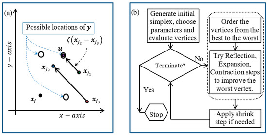
Figure 2.
(a) DE based exploration in (b) Schematic diagram of NMS method.
Appendix A presents pseudo code of the order of DE-NMS operations and Figure 3 exhibits complete schematic diagram of EPA method.
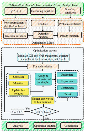
Figure 3.
Schematic diagram of EPA scheme.
4. Results and Discussion
The solutions of the dimensionless coupled system of Equations (4)–(7) with boundary conditions (8) have been found by optimizing objective function given by Equation (31) in the EPA environment. Some fundamental calculations can be helpful in reducing the dimensions of vector of decision variables. To this end, we apply boundary conditions on approximate solutions with the following general properties of Padé approximants:
The constraints defined by Equations (19)–(23) at imply that:
The constraints defined by Equations (24)–(27) with imply that:
The above calculations directly imply a reduction in the number of decision variables by nine. Hence, the problem dimensions are reduced to .
Equations (32)–(35) imply that the initial as well infinity boundary conditions are exactly satisfied by the rational approximation functions. The next component of the used method is the minimization of the objective function (31) to some acceptable tolerance. Such optimization process is essential to guarantee the fulfillment of governing Equations (4)–(7) by Padé approximants within the domain of the similarity variable. For this purpose, the optimization process of DE-NMS optimizer is executed up to iterations with algorithmic parameters set as , , and . It has been found that the minimized objective function value less the captures the dynamics of the model efficiently. The corresponding sub-sections contain convergence graphs displaying the minimization progress for the obtained solutions.
The dynamics of the heat transfer, mass transfer, and flow of bio-convective Casson fluid past a wedge have been thoroughly investigated considering the impact of several combinations of values of governing physical parameters. In order to validate the numerical accuracy, the computed values of the local Nusselt number and the coefficient of skin friction have been compared to past work with respect to various values of the Falkner–Skan power-law parameter. From Table 1, it is evident that the results produced by the utilized approach and those published by Raju and Sandeep [27] and Kou [48] are in excellent agreement. Similarly, Table 2 shows that the skin friction coefficient values obtained by the EPA scheme agree well with those reported in the literature [18,28,49]. Thus, we are confident that the results reported here are accurate.

Table 1.
Comparison of the local Nusselt number for different values of when , .
Table 2.
Comparison of the skin friction coefficient () for different values of when .
The dimensionless parameters linked to MHD flows can be varied in a wide range of values, but to fulfill the restrictions of the mathematical model, it is acceptable to consider appropriate combinations of the dimensionless parameters for analysis purpose [50]. Therefore, as in reference [28], the values of dimensionless parameters , , , , , , , , , and are fixed as 1, 0.5, 0.2, 0.3, 0.2, 0.2, 0.2, 0.2, 4, and 1, respectively, as general setting, but exactly one of these parameters varies for observing its impact.
4.1. Dynamics of Velocity Profiles
The dynamics of velocity profiles have been investigated with respect to Casson fluid viscosity force parameter (), magnetic field parameter (), and fluid flow parameter in the Falkner–Skan sense, considering three scenarios (, , , , , , , ,, ). Employing Equations (34) and (35), the closed forms of approximate solutions obtained by EPA scheme are presented in Equations (36)–(44).
The convergence curves of optimization process of all scenarios are presented in parts of Figure 4. The residuals in all three cases were reduced up to . At these optimization results, the EPA scheme was able to clearly distinguish the impacts of physical parameters , and . Figure 5 demonstrates that the velocity profiles increase when a decrease in viscosity force parameter occurs.
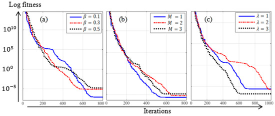
Figure 4.
Convergence curves of optimization process for velocity profiles with respect to variations in (a) Casson fluid viscosity force parameter (b) Magnetic field parameter (c) Hartree pressure gradient parameter.
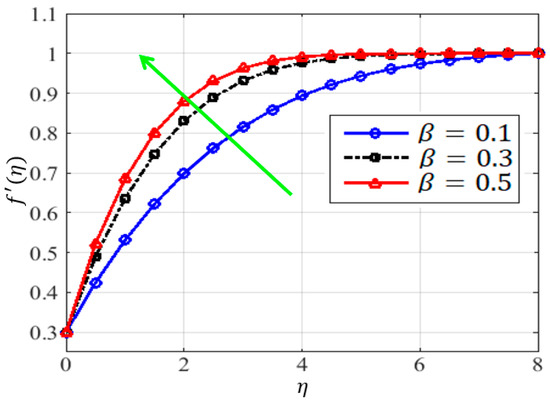
Figure 5.
Impact of Casson fluid viscosity force parameter on velocity profile.
Figure 6 shows that velocity profiles are positively influenced by the magnetic field parameter, i.e., increasing values of cause an increase in velocity profiles. The effect of fluid flow parameter on velocity profiles has been presented in Figure 7. One can observe that velocity profiles are increased when the values of are increased.
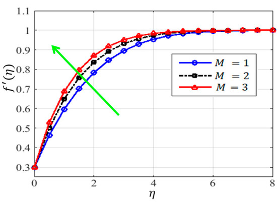
Figure 6.
Impact of magnetic field parameter on velocity profile.
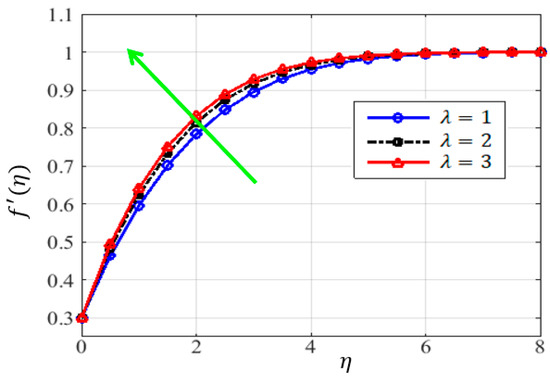
Figure 7.
Impact of fluid flow parameter on velocity profile.
4.2. Dynamics of Temperature Field
The dynamics of temperature field have been investigated with respect to radiation parameter (), Prandtl number (), and thermophoresis parameter , considering the scenarios (, , , , , ,, , , ). Equations (45)–(53) present the approximate solutions with respect to considered scenarios. The convergence curves of optimization process up to 1000 iterations of all scenarios are presented in Figure 8.
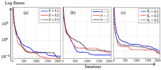
Figure 8.
Convergence curves of optimization process for temperature field with respect to variations in (a) Radiation parameter (b) Prandtl number (c) Thermophoresis parameter.
The impact of radiation parameter () on temperature field is plotted in Figure 9. The physical behavior of fluid is greatly affected by variations in the thermal radiation parameter. The incremental values of the parameter of thermal radiation support internal heat energy during the flow. Due to this, the temperature profile is driven to increase. The graphical view of impact of Prandtl number () on temperature profile is presented in Figure 10. It can be observed that the increasing values of have reverse influence on temperature profile. Figure 11 demonstrates that the increase in values of thermophoresis parameter () impacts the temperature field.
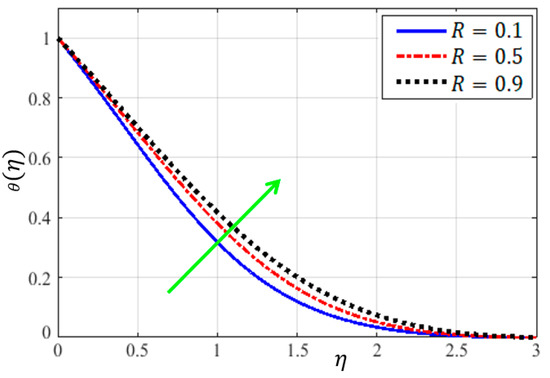
Figure 9.
Impact of radiation parameter on temperature field.
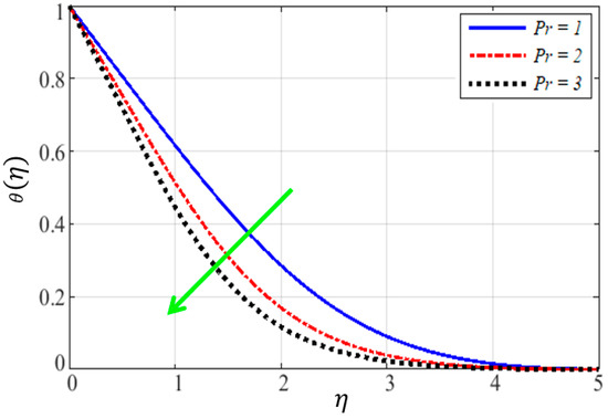
Figure 10.
Impact of Prandtl number on temperature field.
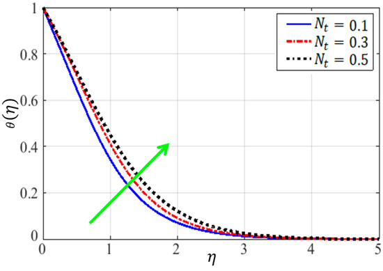
Figure 11.
Impact of thermophoresis parameter on temperature field.
4.3. Dynamics of Fluid Concentration Fields
The dynamics of temperature field have been investigated with respect to magnetic field parameter (), thermophoresis parameter (), fluid parameter (), and considering the scenarios (, , , , , , , , , ). The convergence curves of optimization process of scenarios are similar to those of Figure 8. The optimized approximate solutions with respect to variations in magnetic field parameter (), presented below by Equations (54)–(56), are plotted in Figure 12.
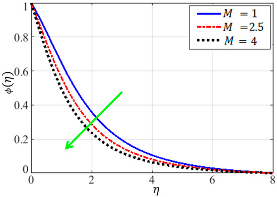
Figure 12.
Impact of magnetic field parameter on fluid’s concentration.
From Figure 12, it is observed that small variations in values of in vicinity of four are not able to distinguish its impact on fluid concentration field; therefore, comparatively larger variations have been used to visualize the inverse effects of increasing values of on fluid’s concentration field. The analytical forms of solutions for different values of are presented by Equations (57)–(59) and are plotted in Figure 13. It is evident that increasing values of parameter cause an increase in concentration profile. Equations (60)–(62) present the analytical solutions related to the values of Casson flow viscosity parameter and are plotted in Figure 14. Clearly, a decrease in concentration profile is observed with increasing values of .
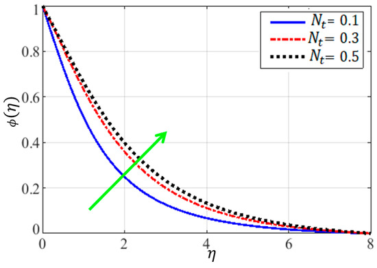
Figure 13.
Impact of thermophoresis parameter on fluid’s concentration field.
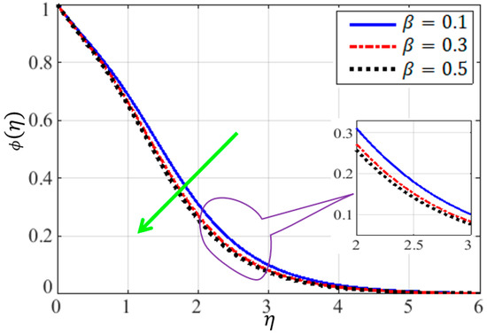
Figure 14.
Impact of Casson fluid viscosity force parameter on fluid’s concentration field.
4.4. Dynamics of Density of Motile Organisms
The dynamics of density of motile organisms have been investigated with respect to Casson fluid viscosity force parameter (), Péclet number (), and fluid parameter (), considering the scenarios (, , , , , , , , , ). The convergence curves of optimization processes are presented in Figure 15. The optimized approximate solutions with respect to variations in parameter are expressed in Equations (63)–(65) and plotted in Figure 16.
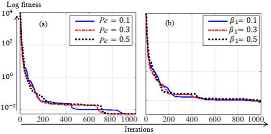
Figure 15.
Convergence curves of optimization process for (a) concentration and (b) density fields.
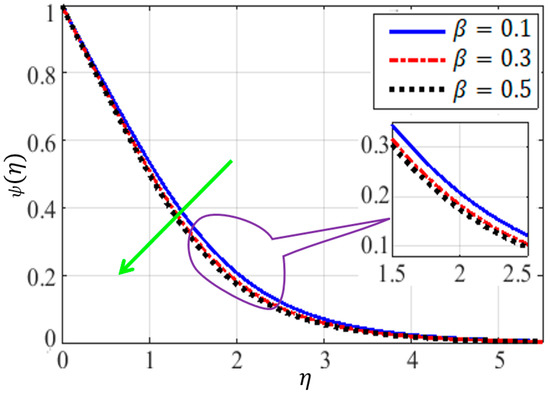
Figure 16.
Impact of radiation parameter on density profile of microorganism.
It can be observed from Figure 16 that the increasing values of Casson fluid viscosity parameter apply decreasing effects on concentration of motile organisms.
The solutions expressed in Equations (66)–(71) plotted in Figure 17 and Figure 18. Figure 17 demonstrates that the increase in the Péclet number () causes a decrease in motile microorganisms’ density. This fact is because of unbalanced ratio between time scales. Figure 18 exhibits the influence of on the density of microorganisms. The increasing values of sfluid parameter () also decrease the density profiles of motile microorganism. It is important to note that the density field of microorganism in the Falkner–Skan flow is low when i.e., the flow turns to be the Blasius. The results also revealed that the increments in magnetic field parameter () cause a decrease in density profile of microorganism.
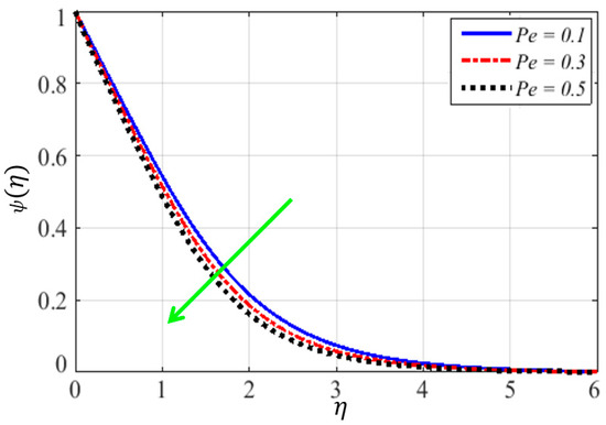
Figure 17.
Impact of Péclet number on microorganism density field.
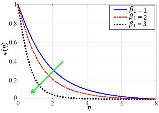
Figure 18.
Impact of fluid parameter on microorganism density field.
5. Conclusions
In this work, an evolutionary framework based on Padé rational functions and a hybrid metaheuristic have been proposed for investigating the dynamics of velocity profiles, heat transfer, fluid concentration field, and density profile of motile microorganisms in the Falkner–Skan flow of a bio-convective Casson fluid over a wedge filled with gyrotactic microorganisms. The convergent aspects of Padé approximations are successfully employed to handle asymptotic boundary conditions. The effects of physical parameters were efficiently computed by the EPA scheme with respect to several combinations of parameters. A comparative study shows good agreement of computed results with those reported in the past studies. The main findings of this study are listed below.
- The governing equation of the velocity profile involves three physical parameters: Casson fluid viscosity force parameter (), magnetic field parameter (), and fluid flow parameter (). The velocity profile increases when each of these parameters is increased.
- Heat transfer rate increases with the increasing values of the radiation parameter () and thermophoresis parameter (), whereas it decreases with the increasing values of the Prandtl number ().
- When the magnetic field parameter () and Casson fluid viscosity force parameter () are increased, the fluid concentration field drops. On the other hand, when the thermophoresis parameter () is increased, the fluid concentration field increases.
- Finally, when the Péclet number () increases, the density field of motile microorganisms decreases; however, as the radiation parameter () and Prandl number () increase, the density field continues to increase as well.
Author Contributions
Conceptualization, J.A.; Methodology, G.A.B. and J.A.; Formal analysis, G.A.B.; Investigation, G.A.B.; Writing—original draft, J.A.; Writing—review & editing, N.R.; Visualization, N.R.; Supervision, N.R.; Funding acquisition, G.A.B. All authors have read and agreed to the published version of the manuscript.
Funding
This research work was funded by Institutional Fund Projects under grant no. (IFPIP: 879-247-1443). The authors gratefully acknowledge technical and financial support provided by the Ministry of Education and King Abdulaziz University, DSR, Jeddah, Saudi Arabia.
Data Availability Statement
Not applicable.
Conflicts of Interest
The authors declare no conflict of interest.
Nomenclature
| Velocity components (m/s). | |
| Temperature of the fluid (K) | |
| Concentration of the fluid (Moles/kg) | |
| Density of motile micro organisms | |
| , | Space coordinates (m). |
| , | Specific heat capacity at constant pressure (J/Kg K) |
| Velocity component of the fluid at the wedge | |
| Temperature of the fluid at the wedge | |
| Concentration of the fluid at the wedge | |
| Velocity component of the fluid at the free stream | |
| Temperature of the fluid at the free stream | |
| Concentration of the fluid at the free stream | |
| Free stream velocity | |
| Coefficient of thermophoresis diffusion | |
| Coefficient of thermophoretic diffusion | |
| Varying magnetic field | |
| Magnetic induction parameter | |
| Density of coefficient of diffusion | |
| Maximum swimming speed of the cell | |
| Chemotaxis coefficient | |
| Acceleration due to gravity (m/s2) | |
| Electrical conductivity () | |
| Fluid heat capacity (Kg/m3K) | |
| Effective heat capacity of particle (Kg/m3K) | |
| Density of the fluid (kg/m3) | |
| Thermal conductivity of the fluid | |
| Subscripts | |
| ,y | Partial derivatives |
| Conditions at the wedge and free stream, respectively. | |
| All other subscripts denote physical constants. | |
| Dimensionless parameters | |
| Péclet number | |
| Prandtl number | |
| Lewis number | |
| Brownian motion parameter | |
| Thermophoresis parameter | |
| Radiation parameter | |
| Magnetic field parameter | |
| Parameter of Falkner–Skan power law | |
| Hartree pressure gradient parameter | |
| Casson fluid viscosity force parameter | |
| Fluid parameter | |
| Wedge parameter | |
| Dimensionless variables | |
| Similarity variable | |
| Velocity profile | |
| Temperature profile | |
| Fluid concentration profile | |
| Motile microorganism density | |
| Others | |
| Kinematic viscosity of the fluid | |
| Specific heat capacitance | |
| Effective heat capacity of the fluid phase with respect to the particle | |
| Base fluid’s density | |
| Aggregate absorption coefficient | |
| Stefan-Boltzmann coefficient | |
| Dynamic viscosity of base fluid | |
| Derivative with respect to similarity variable | |
Appendix A
| Pseudo code of DE-NMS algorithm |
| Step I: Initialization |
|
| , , store the best solution as . |
|
| Step II: //DE phase // |
| For each , choose distinct integers . Set . |
|
| Step III: // NMS phase// |
|
| Step IV: Display results: Display as optimum solution of problem (38) and Stop. |
References
- Harris, J. Rheology and Non-Newtonian Flow; Longman: New York, NY, USA, 1977; pp. 28–33. [Google Scholar]
- Bird, R.B.; Curtis, C.F.; Armstrong, R.C.; Hassager, O. Dynamics of Polyometric Liquids; Wiley: New York, NY, USA, 1987. [Google Scholar]
- Batchelor, B.G.K. The effect of Brownian motion on the bulk stress in a suspension of spherical particles. J. Fluid Mech. 1977, 83, 97–117. [Google Scholar] [CrossRef]
- Hillesdon, A.J.; Pedley, T.J.; Kessler, J.O. The development of concentration gradients in a suspension of chemotactic bacteria. Bull. Math. Biol. 1995, 57, 299. [Google Scholar] [CrossRef]
- Guell, D.C.; Brenner, H.; Frankel, R.B.; Hartman, H. Hydrodynamic forces and band formation in swimming magnetotactic bacteria. J. Theor. Biol. 1988, 135, 525. [Google Scholar] [CrossRef]
- Alloui, Z.; Nguyen, T.H.; Bilgen, E. Bioconvection of gravitactic microorganisms in a vertical cylinder. Int. Commun. Heat Mass Transf. 2005, 32, 739–747. [Google Scholar] [CrossRef]
- Ishikawa, T.; Pedley, T.J. The rheology of a semi-dilute suspension of swimming model micro-organisms. J. Fluid Mech. 2007, 588, 399–435. [Google Scholar] [CrossRef]
- Mehandia, V.; Nott, P.R. The collective dynamics of self-propelled particles. J. Fluid Mech. 2008, 595, 239–264. [Google Scholar] [CrossRef]
- Pedley, T.J. Instability of uniform micro-organism suspensions revisited. J. Fluid Mech. 2010, 647, 335–359. [Google Scholar] [CrossRef]
- Nguyen-quang, T.R.I.; Guichard, F. The role of bioconvection in plankton population with thermal stratification. Int. J. Bifurc. Chaos 2010, 20, 1761–1778. [Google Scholar] [CrossRef]
- Ghorai, S.; Panda, M.K.; Hill, N.A. Bioconvection in a suspension of isotropically scattering phototactic algae. Phys. Fluids 2010, 22, 071901. [Google Scholar] [CrossRef]
- Kuznetsov, A.V. Bio-thermal convection induced by two different species of microorganisms. Int. Commun. Heat Mass Transf. 2011, 38, 548–553. [Google Scholar] [CrossRef]
- Hayat, T.; Hussain, M.; Nadeem, S.; Mesloub, S. Falkner–Skan wedge flow of a power-law fluid with mixed convection and porous medium. Comp. Fluids 2011, 49, 22–28. [Google Scholar] [CrossRef]
- Rashidi, M.M.; Rastegari, M.T.; Asadi, M.; Bég, O.A. A study of non-Newtonian flow and heat transfer over a non-isothermal wedge using the homotopy analysis method. Chem. Eng. Commun. 2011, 199, 231–256. [Google Scholar] [CrossRef]
- Khan, W.A.; Pop, I. Boundary layer flow past a wedge moving in a nanofluid. Math. Probl. Eng. 2013, 2013, 637285. [Google Scholar] [CrossRef]
- Nadeem, S.; Haq, R.U.; Akbar, N.S. MHD three-dimensional boundary layer flow of Casson nanofluid past a linearly stretching sheet with convective boundary condition. IEEE Trans. Nanotechnol. 2014, 13, 109–115. [Google Scholar] [CrossRef]
- Raju, C.S.K.; Sandeep, N. Heat and mass transfer in MHD non-Newtonian bio-convection flow over a rotating cone/plate with cross diffusion. J. Mol. Liq. 2016, 215, 115–126. [Google Scholar] [CrossRef]
- Mukhopadhyay, S.; Mondal, I.C.; Chamkha, A.J. Casson fluid flow and heat transfer past a symmetric wedge. Heat Transf. Asian Res. 2013, 42, 665–675. [Google Scholar] [CrossRef]
- Animasaun, I.L.; Raju, C.S.K.; Sandeep, N. Unequal diffusivities case of homogeneous–heterogeneous reactions within viscoelastic fluid flow in the presence of induced magnetic-field and nonlinear thermal radiation. Alex. Eng. J. 2016, 55, 1595–1606. [Google Scholar] [CrossRef]
- Raju, C.S.K.; Sandeep, N. Unsteady three-dimensional flow of Casson–Carreau fluids past a stretching surface. Alex. Eng. J. 2016, 55, 1115–1126. [Google Scholar] [CrossRef]
- Uddin, M.J.; Kabir, M.N.; Bég, O.A. Computational investigation of Stefan blowing and multiple-slip effects on buoyancy-driven bio-convection nanofluid flow with microorganisms. Int. J. Heat Mass Transf. 2016, 95, 116–130. [Google Scholar] [CrossRef]
- Dhanai, R.; Rana, P.; Kumar, L. Lie group analysis for bio-convection MHD slip flow and heat transfer of nanofluid over an inclined sheet: Multiple solutions. J. Taiwan Inst. Chem. Eng. 2016, 66, 283–296. [Google Scholar] [CrossRef]
- Coelho, P.M.; Pinho, F.T.; Oliveira, P.J. Fully developed forced convection of the Phan-Thien–Tanner fluid in ducts with a constant wall temperature. Int. J. Heat Mass Trans. 2002, 45, 1413–1423. [Google Scholar] [CrossRef]
- Francisca, J.S.; Tso, C.P.; Hung, Y.M.; Rilling, D. Heat transfer on asymmetric thermal viscous dissipative Couette–Poiseuille flow of pseudo-plastic fluids. J. Non-Newton. Fluid Mech. 2012, 169–170, 42–53. [Google Scholar] [CrossRef]
- Chamkha, A.J.; Rashad, A.M.; Kameswaran, P.K.; Abdou, M.M.M. Radiation effects on natural bioconvection flow of a nanofluid containing gyrotactic microorganisms past a vertical plate with streamwise temperature variation. J. Nanofluids 2017, 6, 587–595. [Google Scholar] [CrossRef]
- Rashad, A.M.; Chamkha, A.; Mallikarjuna, B.; Abdou, M.M.M. Mixed bioconvection flow of a nanofluid containing gyrotactic microorganisms past a vertical slender cylinder. Front. Heat Mass Transf. 2018, 10, 21. [Google Scholar]
- Rashad, A.M.; Nabwey, H.A. Gyrotactic mixed bioconvection flow of a nanofluid past a circular cylinder with convective boundary condition. J. Taiwan Inst. Chem. Eng. 2019, 99, 9–17. [Google Scholar] [CrossRef]
- Raju, C.S.K.; Sandeep, N. A comparative study on heat and mass transfer of the Blasius and Falkner–Skan flow of a bio-convective Casson fluid past a wedge. Eur. Phys. J. Plus 2016, 131, 405. [Google Scholar] [CrossRef]
- Falkner, V.M.; Skan, S.W. Some approximate solutions of the boundary layer equations. Philos. Mag. 1931, 12, 865–896. [Google Scholar] [CrossRef]
- Thomas, J.W. Numerical Partial Differential Equations: Finite Difference Methods; Springer: New York, NY, USA, 1995. [Google Scholar]
- Hartley, T.; Wanner, T. A semi-implicit spectral method for stochastic nonlocal phase-field models. Discrete Contin. Dyn. Syst. A 2009, 25, 399–429. [Google Scholar] [CrossRef]
- Guo, B.Y.; Shen, J.; Wang, Z.Q. Chebyshev rational spectral and pseudo spectral methods on a semi-infinite interval. Int. J. Numer. Methods Eng. 2002, 53, 65–84. [Google Scholar] [CrossRef]
- Inayat, U.; Iqbal, S.; Manzoor, T. Theoretical investigation of two-dimensional nonlinear radiative thermionics in Nano-MHD for solar insolation: A semi-empirical approach. Comput. Model. Eng. Sci. 2022, 130, 751–776. [Google Scholar] [CrossRef]
- Khan, K.A.; Seadawy, A.R.; Raza, N. The homotopy simulation of MHD time dependent three dimensional shear thinning fluid flow over a stretching plate. Chaos Solitons Fractals 2022, 157, 111888. [Google Scholar] [CrossRef]
- Abdullah, M.; Butt, A.R.; Raza, N.; Haque, E.U. Semi-analytical technique for the solution of fractional Maxwell fluid. Can. J. Phys. 2018, 95, 472–478. [Google Scholar] [CrossRef]
- Abdullah, M.; Butt, A.R.; Raza, N.; Alshomrani, A.S.; Alzahrani, A.K. Analysis of blood flow with nanoparticles induced by uniform magnetic field through a circular cylinder with fractional Caputo derivatives. J. Magn. Magn. Mater. 2018, 446, 28–36. [Google Scholar] [CrossRef]
- Razzaq, A.; Seadawy, A.R.; Raza, N. Heat transfer analysis of viscoelastic fluid flow with fractional Maxwell model in the cylindrical geometry. Phys. Scr. 2020, 95, 115220. [Google Scholar] [CrossRef]
- Babaei, M. A general approach to approximate solutions of nonlinear differential equations using particle swarm optimization. Appl. Soft Comput. 2013, 13, 3354–3365. [Google Scholar] [CrossRef]
- Mastorakis, N.E. Unstable ordinary differential equations: Solution via genetic algorithms and the method of Nelder-Mead. WSEAS Trans. Math. 2006, 5, 1276–1281. [Google Scholar]
- Cao, H.; Kang, L.; Chen, Y. Evolutionary modelling of systems of ordinary differential equations with genetic programming. Genet. Program. Evolvable Mach. 2000, 1, 309–337. [Google Scholar] [CrossRef]
- Panagant, N.; Bureerat, S. Solving partial differential equations using a new differential evolution algorithm. Math. Probl. Eng. 2014, 10, 747490. [Google Scholar] [CrossRef]
- Ali, J.; Saeed, M.; Rafiq, M.; Iqbal, S. Numerical treatment of nonlinear model of virus propagation in computer networks: An innovative evolutionary Padé approximation scheme. Adv. Differ. Equ. 2018, 2018, 214. [Google Scholar] [CrossRef]
- Ali, J.; Raza, A.; Ahmed, N.; Ahmadian, A.; Rafiq, M.; Ferrara, M. Evolutionary optimized Padé approximation scheme for analysis of covid-19 model with crowding effect. Oper. Res. Perspect. 2021, 100207. [Google Scholar] [CrossRef]
- Nisar, K.S.; Ali, J.; Mahmood, M.K.; Ahmad, D.; Ali, S. Hybrid evolutionary Padé approximation approach for numerical treatment of nonlinear partial differential equations. Alex. Eng. J. 2021, 60, 4411–4421. [Google Scholar] [CrossRef]
- Storn, R.; Price, K. Differential evolution—A simple and efficient heuristic for global optimization over continuous spaces. J. Glob. Optim. 1997, 11, 341–359. [Google Scholar] [CrossRef]
- Nelder, J.A.; Mead, R. A simplex method for function minimization. Comput. J. 1965, 7, 308–313. [Google Scholar] [CrossRef]
- Ali, J.; Saeed, M.; Chaudhry, N.A.; Tabassum, M.F.; Luqman, M. Low cost efficient remedial strategy for stagnated Nelder-Mead simplex method. Pak. J. Sci. 2017, 69, 119–126. [Google Scholar]
- Kuo, B.L. Heat transfer analysis for the Falkner–Skan wedge flow by the differential transformation method. Int. J. Heat Mass Transf. 2005, 48, 5036–5046. [Google Scholar] [CrossRef]
- Yih, K.A. MHD forced convection flow adjacent to a non-isothermal wedge. Int. Commun. Heat Mass Transf. 1999, 26, 819–827. [Google Scholar] [CrossRef]
- Escandón, J.; Santiago, F.; Bautista, O.; Méndez, F. Hydrodynamics and thermal analysis of a mixed electro magneto hydrodynamic pressure driven flow for Phan–Thien–Tanner fluids in a microchannel. Int. J. Therm. Sci. 2014, 86, 246–257. [Google Scholar] [CrossRef]


Disclaimer/Publisher’s Note: The statements, opinions and data contained in all publications are solely those of the individual author(s) and contributor(s) and not of MDPI and/or the editor(s). MDPI and/or the editor(s) disclaim responsibility for any injury to people or property resulting from any ideas, methods, instructions or products referred to in the content. |
© 2023 by the authors. Licensee MDPI, Basel, Switzerland. This article is an open access article distributed under the terms and conditions of the Creative Commons Attribution (CC BY) license (https://creativecommons.org/licenses/by/4.0/).