Optimization of Drone Base Station Location for the Next-Generation Internet-of-Things Using a Pre-Trained Deep Learning Algorithm and NOMA

Abstract

Next-generation Internet-of-Things applications pose challenges for sixth-generation (6G) mobile networks, involving large bandwidth, increased network capabilities, and remarkably low latency. The possibility of using ultra-dense connectivity to address the existing problem was previously well-acknowledged. Therefore, placing base stations (BSs) is economically challenging. Drone-based stations can efficiently address Next-generation Internet-of-Things requirements while accelerating growth and expansion. Due to their versatility, they can also manage brief network development or offer on-demand connectivity in emergency scenarios. On the other hand, identifying a drone stations are a complex procedure due to the limited energy supply and rapid signal quality degradation in air-to-ground links. The proposed method uses a two-layer optimizer based on a pre-trained VGG-19 model to overcome these issues. The non-orthogonal multiple access protocol improves network performance. Initially, it uses a powerful two-layer optimizer that employs a population of micro-swarms. Next, it automatically develops a lightweight deep model with a few VGG-19 convolutional filters. Finally, non-orthogonal multiple access is used to schedule radio and power resources to devices, which improves network performance. We specifically examine how three scenarios execute when various Cuckoo Search, Grey Wolf Optimization, and Particle Swarm Optimization techniques are used. To measure the various methodologies, we also run non-parametric statistical tests, such as the Friedman and Wilcoxon tests. The proposed method also evaluates the accuracy level for network performance of DBSs using number of Devices. The proposed method achieves better performance of 98.44% compared with other methods.

1. Introduction

Modern mobile networks will experience an extraordinary rise in demand for computational and networking resources, driven by the next-generation Internet of Things (NG-IoT) growth. Numerous applications, including medical, intelligent buildings, and heavy manufacturing, incorporate NG-IoT. There are more requirements for connecting devices, network capacity, and link latency for these applications. Sixth-generation (6G) networks successfully enable various forms of connectivity [1].

A novel concept known as the drone-base-station (DBS) can effectively aid in meeting the expanding system requirement and permit network coverage [2]. DBSs are flexible systems that improve user throughput, improve QoS, and expand mobile phone network coverage. DBSs can also boost system performance for brief occurrences by relieving congestion or offering connections in emergencies like terrestrial BS failures and environmental catastrophes [3]. Lastly, DBSs may dramatically lower the total amount of money spent by operators of mobile networks because they offer on-demand wireless services [4].

The DBS has limited capacity, so it is essential to use it as well as feasible. Available storage, transmission distance, transmission reflections, and shadows considerably harm the person’s receiver end [5]. The DBS must have high quality to get excellent QoS and a high competency level to prevent the decrease of transmission strength. This has spurred several researchers to formulate and address the DBS optimal location concerns. Specifically, [6] seeks to increase the number of supported users with various QoS needs. The goal of [6] is to accommodate more individuals who have distinct QoS requirements. The DBS placement issue is modeled and resolved via extensive search as a multiple-circle location and sizing. The idea of putting a DBS inside a high-rise building is examined in [7]. The DBS distribution issue is modeled and resolved via extensive search using a multiple-circle optimization method. Ref. [7] investigates where a DBS should be placed in a tall place.

Deep learning recently successfully identified road damage [8,9]. For instance, the backbone network for extracting features with a softmax was a pre-trained convolutional neural network (CNN) model Visual Geometry Group (VGG-16) used by the author [10]. According to reported findings, a collection of photographs of concrete cracks demonstrated a road crack detection performance of 97.8%. Furthermore, for non-drone-obtained photos, the models in [11,12] were used. More crucially, earlier research should have accounted for the increase in model complexity caused by the number of pre-trained networks in the CNN filters, including VGG-19.

The DBS location issue can be solved using swarm intelligence techniques. The efforts have demonstrated the intricacy of the DBS placement challenge. In most of them, the writers tried to approach the issue by decomposing it into more minor, manageable difficulties to develop a more specific path. Also, the writers employed time-consuming search methods in several articles. As a result, in this work, we intend to assess how well-known swarm intelligence techniques perform in locating the ideal DBS under varied goals and constraints. In this approach, we analyze three situations where several Internet of Things (IoT) devices are covered by a single or numerous DBSs, providing wireless coverage. The contributions that this research has made are listed as follows:

✓

The proposed method uses a powerful two-layer optimizer that utilizes the micro-swarm population and has a global and local search layer. It develops a pre-trained lightweight VGG-19 feature extractor with a few convolutional filters.

✓

The two-layer optimizer minimizes path loss among the devices and enhances maximum coverage.

✓

The Multi carrier non-orthogonal multiple access (NOMA) with the simultaneous wireless information and power transfer (SWIPT) method improves the network performance and provides power scheduling to the devices.

✓

We also conduct non-parametric statistical tests to further assess these methods’ effectiveness. Depending on the results of these experiments, we rank the various swarm intelligence methodologies.

The rest of the paper is organized into sections, as shown. Section 2 briefly studies the existing Next Generation Internet of Things and Deep Learning Methods. Section 3 describes the working principle of the proposed model. Section 4 evaluates the result and compares the existing VS presented. Section 5 concludes the research work with the future scope.

2. Related Works

Many wireless applications have used swarm intelligence techniques to solve optimization issues. The author shows a tiny tag transmitter with a high gain and a high distance [13]. The artificial ant colony algorithm was explicitly used to create the tag antenna design the tag antenna The authors [14] optimized a linear antenna array using the spider monkey optimization approach to disrupt side lobes and put nulls in specific direction directions acquired power, the researcher [15] developed a modeling approach. This proposed method generates exact forecasts by combining the salp swarm method with five base classifiers.

The authors used the coyote optimization process in [16] to develop the pattern of a multiband microstrip patch antenna. The author introduced [17] a social network optimization technique for designing beam-scanning reflect array antennas. The method was applied to maximize the propagation characteristics of the various antennas and reduce the discrepancy between the current and desired radiation directions. The author [18] also employed the Adaptive Opposite Fireworks Algorithm to minimize the interference brought on by radar systems ‘authors [19] created a beam-forming method that uses a conformal phased-array radar system to achieve quick data updates.

The author [20] developed an ideal DBS deployment approach that serves a group of ground users while utilizing the least amount of transmit power. The horizontal and vertical placement subproblem optimum DBS placement issues were separated. As an outcome of the computations, it was discovered that the power usage in dense urban, rural, and urban areas had dropped. In [21], the topic of combined installation and system allocation is examined. The deployment of resources problem and the DBS location issue is the authors’ two more minor problems that they identify. The writers thoroughly examine all the potential sites to determine the DBS position that maximizes throughput.

The authors in [22] created analytical formulas for the DBS hovering. An elevation where the energy consumption is optimized. Furthermore, the horizontal positioning issue was handled by applying the multilayer standard polygon-based placement algorithm to a circle packing problem to achieve the highest packing density. The authors mainly emphasized the energy-efficient placement optimization technique [23]. The horizontal and vertical placement issues were dissociated to solve their complexity. Whereas the upright positioning was optimized using a Weiszfeld-based method, the horizontal placement was analytically resolved by utilizing the coverage area’s radius and the ideal elevation angle. Numerous fields, including research, technology, and business, have given swarm intelligence techniques a lot of attention [24,25,26]. The computational intelligence subfield known as “swarm intelligence” focuses on how a species’ population collaborates and is self-organizing. Integrated Sensing and Communications for UAV Communications with Jittering Effect” refers to a system that combines sensing (i.e., data collection) and communication capabilities for unmanned aerial vehicles (UAVs) that experience jittering effects in their flight [27,28,29]. The broadband cancellation method in an adaptive co-site interference cancellation system” is a technique used to remove interference from a co-located (co-site) signal source in a communication system [30]. The technique used to forecast the behavior of a wireless communication channel in a multiple-input multiple-output (MIMO) system. It involves using ordinary differential equations to model the time-varying properties of the network, such as receding and delay and then using the model to predict the channel’s future behavior [31,32]. A Utility-Aware General Framework With Quantifiable Privacy Preservation for Destination Prediction in LBSs” is a general framework for predicting a user’s destination in location-based services (LBS) while preserving their privacy [33]. The analysis considers the impact of generalized fading channels, which can cause signal attenuation and interference [34,35]. The technique involves using energy-harvesting jammers, which are devices that can harvest energy from the received signals and use that energy to generate jamming signals to interfere with eavesdropping attempts [36,37]. The method involves developing synthetic geoelectric data using a mathematical model and a deep neural network to learn the relationship between the geoelectric data and the subsurface resistivity distribution [38,39]. The trained neural network is then used to invert measured geoelectric data to estimate the subsurface resistivity distribution. By combining the advantages of the model-based synthetic geoelectric sampling and deep neural networks, this method provides a faster and more accurate approach to exploring the subsurface resistivity distribution for geological exploration and resource extraction [40,41,42].

LiDAR uses STM32 gating and PMT (Photomultiplier Tube) adjustable gain. STM32 is a microcontroller that enables the gating of the LiDAR system. Gating refers to the technique of controlling the duration of laser pulses, which can improve the accuracy and precision of LiDAR measurements [43]. Waveform decomposition is a technique used to separate the different components of the LiDAR signal, such as the ground and canopy echo. The study aims to identify the most effective algorithm for accurate and efficient decomposition of the LiDAR signal [44]. The paper explicitly considers multiagent systems with antagonistic interactions, which means that the agent’s actions can have opposite effects on the overall design. Additionally, the report finds communication noises, which can affect the accuracy and reliability of information exchange between agents [45]. Ore image classification is used in the mining industry to identify different types of ores based on their visual characteristics. Convolutional neural networks are deep learning algorithms commonly used for image recognition and classification tasks [46]. UAVs have gained popularity recently for their ability to provide wireless communication services in remote areas. However, the limited battery life of UAVs can be a significant challenge for continuous operation [47]. TDD MU-MIMO systems are wireless communication systems that allow multiple users to transmit and receive data simultaneously using multiple antennas. The system is powered wirelessly, meaning the energy required for transmission and reception is obtained from a wireless power source [48,49,50]. Parallel platforms are mechanisms that have multiple arms connected to a base and an end-effector. Six DOF refers to the platform’s ability to move in six different directions, including translation and rotation. The kinematics model is a mathematical representation of the platform’s motion and is used to predict its behavior [51,52].

3. Proposed Methodology

The suggested solution solves the DBS placement problem, which relies on a two-layer optimizer based on a pre-trained VGG-19 model. The recommended approach offers wireless connectivity between IoT devices. The NOMA protocol enhances network performance. Figure 1 shows the architecture diagram of the proposed method.

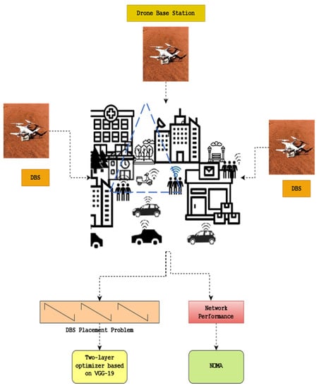
Figure 1. Architecture diagram of the proposed method.

3.1. System Model

A collection of DBSs, indicated by the symbols D = {1,…, D}, connected to various IoT devices, indicated by the symbols S = {1,…, S}. The gadgets are scattered randomly around a territory, and the DBS is hovering over them. The DBS’s floating altitude prevents the links that link it to the ground devices from being accurately characterized using the standard channel models. The given AtG model is employed in determining the LoS chance of an AtG link between the DBS and the S gadget.

$$PA\left(h_d,d{e}_{d,s}\right)=\frac{1}{1+\alpha \exp \left[-\beta \left(\arctan \left(\frac{h_d}{d{e}_{d,s}}\right)-\alpha \right)\right]}$$

(1)

here the environment-based variables are $\alpha$ and $\beta$. Here $d{e}_{d,s}=\sqrt{{(x_d-x_s)}^2+{(y_d-y_s)}^2},$ where ($x_d$, $y_d$) and ($x_s$, $y_s$) are the horizontal positions of the DBS and the devices, correspondingly, and correspondingly, represents the parallel distance among the k-th DBS and the s-th device. The $h_d$ indicates the height of the DBS. The pathloss can therefore be estimated by taking both LoS and non-LoS (NLoS) probability into account.

The IoT devices consist of multiple DBSs linked between the devices, as shown in Figure 1. Initially, it works with a system model and forms the problem.

$$PAL\left(h_d,d{e}_s\right)=20\log \left(\sqrt{h_d^2+d{e}_{d,s}^2}\right)+AP\left(h_d,d{e}_{d,s}\right)+B$$

(2)

where fc is the carrier signal (in Hz), c is the speed of light, LoS and NLoS are the mean extra losses depending on the propagation environment, and A = $\eta LoS$ and $B=20\log \left(\frac{4\pi f_c}{c}\right)$.

3.2. Two-Layer Optimizer Based on Pre-Trained VGG-19

In this work, the two-layer optimizer is used for optimizing the DBS placement issues. It is based on the VGG-19 network. As shown in Figure 2, it essentially comprises two layers: global search and local search. The Q-learning system automatically chooses between local and global search based on the action taken. The following describes the two-layer optimizer’s main phases.

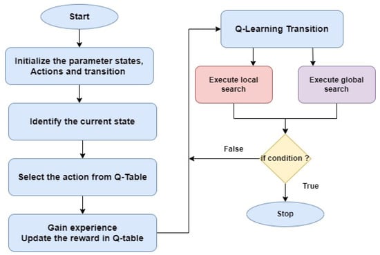
Figure 2. Working flow of the two-layer optimizer.

The two-layer optimizer has four phases, including initialization, transition, searching execution, and terminate condition.

3.2.1. Initialization

The two-stage optimizer’s micro population, which consists of three particles, is initialized during this stage. Based on the DBS problem’s search space, a random initial location is assigned to each particle XP. Each particle also has a velocity value VE that is randomly initialized and whose value falls within the same region as XP.

3.2.2. Transition

A Q-learning algorithm is incorporated at this stage to manage the transition from global search to local search, and vice versa. As stated in [2], when the completed search procedures were successful in improving search performances, the Q-table will be modified with a reward of +1; otherwise, a punishment of −1 is applied.

3.2.3. Searching Execution

In this stage, the search process is carried out between local and global searches. The following equations will be used to update and evolve the micro population of the two-stage optimizer.

$$X{P}_i^{t+1}=X{P}_i^t+V{E}_i^{t+1}$$

(3)

$$V{E}_i^{t+1}=w\ast V{E}_i^t+c_1\ast r_1\left(pBes{t}_i-X{P}_i^t\right)+c_2\ast r_2\left(gBes{t}_i-X{P}_i^t\right)$$

(4)

where VEi denotes particle velocities, w denotes inertia, and $X{P}_i^{t+1}$ denotes time. i represents the new location of the currently active particle i. The social and cognitive acceleration coefficients, c₁ and c₂, are the corresponding variables. The random variables in the range of variables r₁ and r₂ are (0, 1). The micro swarm’s $pBes{t}_i$ and $gBes{t}_i$ values represent their respective best positions attained locally and globally, respectively. The procedures of the global and local searches are similar, but whenever the optimizer runs a local search, just a random subset of the evolving particle’s bins is modified.

3.2.4. Terminating Condition

The maximum allotted iterations must be verified at this stage. If it is met, the two-stage optimizer stops and the best portion of the data obtained by the micro population is released.

The two-layer optimizer based on pre-trained VGG19 is explained below.

A research group from Oxford University created the VGG-19 pre-trained network. With the help of a dataset made up of millions of photos called the ImageNet challenge, VGG-19 was trained. In essence, there are 25 layers that are cascaded. An image with a size of 224 × 224 pixels was intended to be submitted to the input layer. The input image is then sent to three cascading convolutional layers, each of which has 64 filters with a size of 3 pixels. The nonlinearity of the VGG-19 is enhanced by applying a ReLU activation function after each convolutional step.

$$relu\left(x\right)=\max \left(x,0\right)$$

(5)

The result of the relu(x) function is then transferred to the max-pooling layer, wherein x is the number of the pixel. The two-layer optimizer based on the pre-trained VGG-19 network is shown in Figure 3.

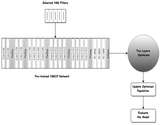
Figure 3. Two-layer optimizer based on the VGG19 network.

3.3. Improving Device Coverage and Minimizing the Pathloss Using Non-Orthogonal Multiple Access (NOMA)

In order to improve device coverage, this work uses multi-carrier NOMA with SWIPT. It schedules the radio and power resources in the DBS system. It also minimizes the path loss between multiple access of IoT devices.

In the downlink SWIPT-enabled MC-NOMA system under consideration, a base station (BS) and K users are superposed on N sub-carriers using pattern division multiple access (PDMA) technology. One single antenna is supposed to be installed on the transmitter and every receiver. Let us use the notation K for all user indices and N for all sub-carrier indices to distinguish them from one another. The overall bandwidth B is equally split into N subcarriers, and each subchannel’s bandwidth is indicated by Bc = B/N. According to the orthogonal frequency division, it is presumed that there is no interference among various subchannels.

The design concepts of PDMA equalize diversity at the reception side while un-equalizing it at the transmitter side. It is more convenient to refer to the mapping of the broadcast signal to a set of subcarriers as an N*K characteristic pattern matrix, or $Q_{PDMA}ϵN^{N\ast K}$. The $Q_{PDMA}{q}_{n,k}=1$ in the n-th row and k-th column indicates that the signal sent to the k-th devices is superposed on the n-th subcarrier (REn), in contrast to q_n,k = 0, which signals the opposite.

$$Q_{PDM{A}^{\left(4,6\right)}=\begin{array}{ccc}1& 0& 0\\ 0& 1& 0\\ 0& 0& 1\end{array}}$$

(6)

The transmission power allotted to the DEk on REn is designated as P_n,k. Consequently, the signal that DEk received via REn can be represented as

$$y_{n,k}=h_{n,k}\left(q_{n,k}\sqrt{P_{n,k},x_{n,k}}+{\displaystyle \sum }_{\begin{array}{c}j\in K\\ j\notin k\end{array}}{q}_{n,j}\sqrt{P_{n,j},x_{n,j}}\right)+z_{n,k}$$

(7)

where $h_{n,k}=g_{n,k}{d}_k^{\beta }$ denotes the small-scale fading and follows a Rayleigh distribution with unit variance and dk represents the channel coefficients from the DBS to DEk via REn. x_n,k (x_n,j) is the information symbol transferred from the BS to DEk (URj) through subcarrier REn with unit energy $\mathbb{E}|\left|x_{n,k}{|}^2,\mathbb{E}\right||x_{n,j}{|}^2$, and $z_{n,k}~CN\left(0,{\sigma }_n^2\right)$ is the additive white Gaussian noise (AWGN) on REn. The dk signifies the large-scale fading. For ease of notation, the channel coefficient is normalised as ${\tilde{h}}_{n,k}=|h_{n.k}{|}^2/{\sigma }_n^2$, which is then defined as the channel-to-noise ratio (CNR).

In view of this, the signal-to-interference plus noise (SINR) of DEk on REn can be expressed as

$${\gamma }_{n.k}=\frac{{\tilde{h}}_{n,k}{q}_{n,k}{P}_{n,k}}{1+I_{n,k}}$$

(8)

In actuality, the breakdown of the SIC procedure will result in outage if the SINR does not satisfy the minimum SINR threshold. We need to meet the following needs to prevent this outage:

$${\gamma }_{n,k}\ge \overline{\gamma },{\forall }_n\in N,{\forall }_k\in {\mathcal{N}}_n$$

(9)

In this circumstance, the DEk on REn available data rate can be expressed as

$$R_{n,k}=B_{c}lo{g}_2\left(1+{\gamma }_{n,k}\right)$$

(10)

The data rate of a device grows as its corresponding signal power rises, according to Shannon’s formula, if the network frequency and noise remain constant. The path loss that the wireless channel experiences determines the received power at a ground device and can be estimated as

$$P{O}_s^{t^{·}}=P{O}_k^t-PAL\left(h_d,d_s\right)-PON$$

(11)

where PON is the strength of the additive white Gaussian noise and $P{O}_k^t$ is the transmission power of the k-th DBS (AWGN). For all of the devices situated in a specific area, the AWGN power will effectively remain the same. As a result, the effect of noise on choosing the ideal D-RRH site will be minimal. To maintain flexibility, we consider PON = 0.

Given a constant transmission power $P{O}_k^t$, the received power can be increased by decreasing the distance-dependent pathloss between DBS and the devices. To reduce the average pathloss of the devices, we optimize the positioning of the DBS in this area. The optimization problem is defined as follows, considering that each device is linked to the closest DBS:

$$minimize\frac{{{\displaystyle \sum }}_{D=1}^D{{\displaystyle \sum }}_{S=1}^{S}PAL\left(h_d,d{e}_s\right)}{S}$$

(12)

4. Experimental Result

We conducted in-depth Monte Carlo simulations to assess the execution of all the above methods, and the finalized results have been generated by combining 1000 trials [1]. The suburban, urban, dense urban, and high-rise urban environments are the four propagation settings that are considered. In Table 1, the propagation parameters for each environment are shown.

Table 1. Factors for propagation in various contexts.

Contexts	$\mathit{\alpha }$	$\mathit{\beta }$	${\mathit{\eta }}_{\mathit{L}\mathit{o}\mathit{S}}$	${\mathit{\eta }}_{\mathit{N}\mathit{L}\mathit{o}\mathit{S}}$
Urban	9.72	0.15	1	20
Suburban	4.58	0.42	0.1	21
Dense Urban	12.07	0.11	1.5	23
High-Rise Urban	27.12	0.07	2.1	32

The proposed method uses three different scenarios with single DBS and multiple DBS. The simulation environment for Scenario 1 is given in Table 2.

Table 2. Simulation parameters for Scenario 1.

Simulation Parameter	Values
Area	1 Km2
Total number of devices used	10, 20, 30, 40, 50
Search agents	5, 25, 50, 75, 100
Total number of generations used	10, 50, 100, 200, 500
Carrier frequency	2.0 Ghz
Environments used	Urban, Suburban, Dense Urban, High-Rise Urban

For evaluating the two-way optimizer with NO-MA methods, we examine three scenarios. If a single DBS is floating above the gadgets in the first scenario, we assess the degree to which the method minimizes average path loss while accounting for variables like the quantity of gadgets, the amount of candidate solutions, the number of generations, and the propagating environment. In the second and third scenarios, we assume that a sizable number of DBS are orbiting a range of gadgets dispersed across a large area. We assess the two-way optimizer with NOMA algorithms in the second scenario to minimize the average path loss for different numbers of DBS and, in the third instance, to maximize the coverage for other DBS.

4.1. Scenario 1: Average Pathloss Using a Single DBS

There are 10, 20, 30, 40, and 50 equally distributed grounded devices in this scenario, which involves a single DBS suspending a group of gadgets over a 1 km² area. The population of search agents and the maximal production for every method are fixed at 10, 50, 100, 200, and 500, respectively. The simulation settings for the first scenario are listed in brief in Table 2.

The proposed method TW-NOMA is compared to existing methods such as CS, GWO, and PSO.

When 20 devices are deployed in an urban setting, and there are a maximum of 100 generations; Figure 4 displays the average pathloss owing to the number of search agents—specific features of CS, GWO, and PSO represent the most fantastic display. CS, GWO, and PSO contain nearly no difference in performance, regardless of the number of search personnel. On the other hand, the TW-NOMA and PSO techniques perform differently depending on the number of search agents. The performance of TW-NOMA improves with more search agents.

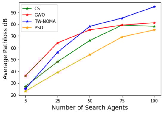
Figure 4. Average pathloss with search agents for Scenario 1.

The total path loss is displayed in Figure 5 as a percentage of the maximum cycles, with a total of 25 searching agents and 20 gadgets, respectively, in an urban environment. The method performs similarly after 100, 200, and 500 iterations, according to the findings. The method performs worse if there are only 10 or 50 iterations, though. As additional generations are used to match the goal more closely, this is to be assumed. The overall quality of TW-NOMA is identical; however, CS and GWO performed the least well and the second worst, accordingly.

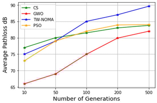
Figure 5. Average pathloss with number of generations for Scenario 1.

4.2. Scenario 2: Average Pathloss Based on Multiple DBSs

In this case, many DBSs are used to provide connectivity as we assess the likelihood of coverage over many devices spread out over a larger area. If a device’s observed path loss is less than a certain threshold, it is regarded as being out of service is shown in Figure 6. The region is 5 km², there are 100 devices, and there are between 1 and 10 DBSs. Moreover, 90, 100, 110, and 120 dB are specified as the threshold values. Additionally, each method has a population of 25 search agents and a maximum generation size of 100. Table 3 provides a summary of the model parameters for the second scenario.

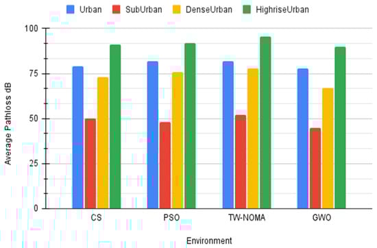
Figure 6. Average pathloss with various environments for Scenario 1.

Table 3. Simulation parameters used for Scenario 2.

Simulation Parameter	Values
Area	5 Km2
Total number of devices used	100
Search agents	25
Total number of generations used	100
Carrier frequency	2.0 Ghz
Environments used	Urban, Suburban, Dense Urban, High-Rise Urban

Figure 7a–d depicts the average pathloss as a function of the number of DBSs in different contexts. In every instance, the average pathloss decreases as the number of DBSs rises. This is to be expected because additional DBSs allow for closer deployment to the devices, which lowers pathloss. The findings show that TW-NOMA performs the best generally, whereas GWO performs worse overall. In all other circumstances, CS and PSO perform similarly. The suburban and high-rise urban environments, which were also inferred from the first scenario, have had the highest and lowest average pathlosses, respectively.

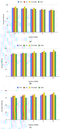
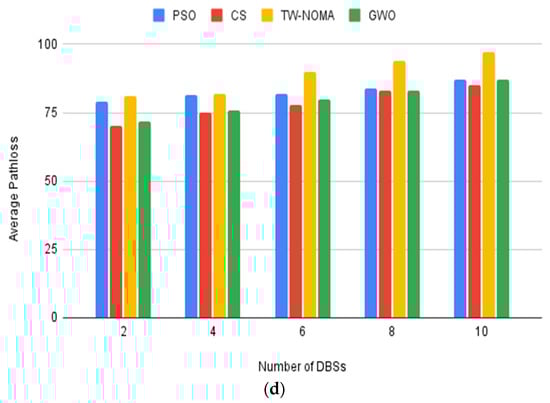
Figure 7. (a) Average pathloss for the urban environment; (b) Average pathloss for the suburban environment; (c) Average pathloss for the dense urban environment; (d) Average pathloss for the high-rise urban environment.

4.3. Scenario 3: Probability Coverage Using Multiple DBSs

In this case, many DBSs are used to offer connections as we assess the likelihood of coverage over many devices spread out over a larger area. If a device’s observed pathloss is less than a certain threshold, it is regarded as being under coverage. The area is 5 km², there are 100 devices, and there are between 1 and 10 DBSs. Moreover, 90, 100, 110, and 120 dB are specified as the threshold values. Additionally, each method has a population of 25 search agents and a maximum generation size of 100. Table 4 provides a summary of the model parameters for the third scenario.

Table 4. Simulation parameters used for Scenario 3.

Simulation Parameter	Values
Area	5 Km2
Total number of devices used	100
Search agents	25
Thresholds	90, 100, 110, 120 dB
Number of generations	100
Carrier frequency	2.0 Ghz
Environments used	Urban, Suburban, Dense Urban, High-Rise Urban

Figure 8, Figure 9, Figure 10 and Figure 11 show the coverage probability owing to the number of DBSs for different criteria. An increase in coverage as the number of DBSs increases is as expected because more devices can be covered by the DBSs when they are dispersed over a larger region. Lower threshold results correspond to reduced coverage probabilities in terms of the threshold. This is to be expected because devices closer to DBSs will have pathloss that is lower than the threshold. Overall, more DBSs are required to preserve a good coverage probability when the threshold is set at 90 dB.

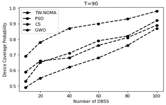
Figure 8. Coverage probability for the urban environment using a threshold of T = 90.

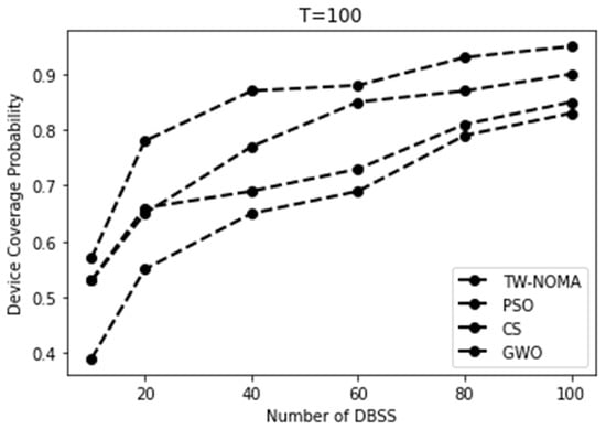
Figure 9. Coverage probability for the sub-urban environment using a threshold of T = 100.

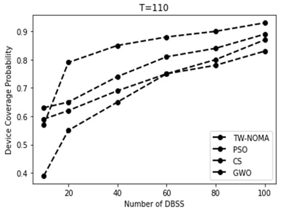
Figure 10. Coverage probability for the dense urban environment using a threshold of T = 110.

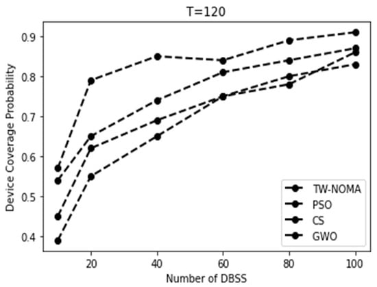
Figure 11. Coverage probability for the high-rise urban environment using a threshold T = 120.

The proposed method also evaluates the accuracy level of the network performance of DBSs using the number of devices. The proposed method achieves better performance compared with other methods. Figure 12 shows the experimental results of accuracy.

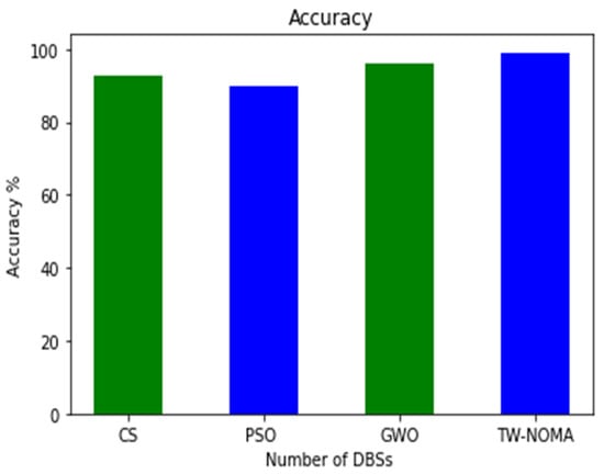
Figure 12. Accuracy of various optimizers compared to the proposed model.

5. Conclusions

We explored the effectiveness of swarm intelligence approaches for optimizing the DBS deployment, which was inspired by the development of NG-IoT and the constraints associated with enormous connectivity. Based on a pre-trained VGG-19 model, the suggested technique employs a two-layer optimizer to circumvent these problems. The non-orthogonal multiple access (NOMA) protocol enhances network performance. Initially, it uses a population of micro-swarms in a powerful two-layer optimizer. The process then automatically creates a shallow model that is not too complex using a few VGG-19 convolutional filters. Finally, NOMA assigns radio and power resources to devices, which improves network performance. The proposed TW-NOMA method improves network coverage while minimizing pathloss between devices. These methods were specifically assessed and contrasted to identify the best DBS sites while employing a variety of criteria, including the number of search agents, the number of maximal generations, the propagating environment, the number of devices, and the area size.

Future research could explore how swarm intelligence and NOMA could be used to optimize other wireless communication systems, such as cellular networks, Wi-Fi hotspots, or ad hoc networks.

References

- Pliatsios, D.; Goudos, S.K.; Lagkas, T.; Argyriou, V.; Boulogeorgos, A.A.A.; Sarigiannidis, P. Drone-base-station for next-generation internet-of-things: A comparison of swarm intelligence approaches. IEEE Open J. Antennas Propag. 2021, 3, 32–47. [Google Scholar] [CrossRef]
- Luo, J.; Tang, J.; So, D.K.; Chen, G.; Cumanan, K.; Chambers, J.A. A deep learning-based approach to power minimization in multi-carrier NOMA with SWIPT. IEEE Access 2019, 7, 17450–17460. [Google Scholar] [CrossRef]
- Kelli, V.; Sarigiannidis, P.; Argyriou, V.; Lagkas, T.; Vitsas, V. A cyber resilience framework for NG-IoT healthcare using machine learning and blockchain. In Proceedings of the ICC 2021—IEEE International Conference on Communications, Montreal, QC, Canada, 14–23 June 2021; pp. 1–6. [Google Scholar]
- Siniosoglou, I.; Sarigiannidis, P.; Argyriou, V.; Lagkas, T.; Goudos, S.K.; Poveda, M. Federated intrusion detection in NG-IoT healthcare systems: An adversarial approach. In Proceedings of the ICC 2021—IEEE International Conference on Communications, Montreal, QC, Canada, 14–23 June 2021; pp. 1–6. [Google Scholar]
- Chen, C.W. Internet of video things: Next-generation IoT with visual sensors. IEEE Internet Things J. 2020, 7, 6676–6685. [Google Scholar] [CrossRef]
- Beliatis, M.J.; Jensen, K.; Ellegaard, L.; Aagaard, A.; Presser, M. Next generation industrial IoT digitalization for traceability in metal manufacturing industry: A case study of industry 4.0. Electronics 2021, 10, 628. [Google Scholar] [CrossRef]
- Bajracharya, R.; Shrestha, R.; Ali, R.; Musaddiq, A.; Kim, S.W. LWA in 5G: State-of-the-art architecture, opportunities, and research challenges. IEEE Commun. Mag. 2018, 56, 134–141. [Google Scholar] [CrossRef]
- Zhang, K.; Zhu, Y.; Maharjan, S.; Zhang, Y. Edge intelligence and blockchain empowered 5G beyond for the industrial Internet of Things. IEEE Netw. 2019, 33, 12–19. [Google Scholar] [CrossRef]
- Mozaffari, M.; Kasgari, A.T.Z.; Saad, W.; Bennis, M.; Debbah, M. Beyond 5G with UAVs: Foundations of a 3D wireless cellular network. IEEE Trans. Wirel. Commun. 2019, 18, 357–372. [Google Scholar] [CrossRef]
- Naqvi, S.A.R.; Hassan, S.A.; Pervaiz, H.; Ni, Q. Drone-aided communication as a key enabler for 5G and resilient public safety networks. IEEE Commun. Mag. 2018, 56, 36–42. [Google Scholar] [CrossRef]
- Sharma, N.; Magarini, M.; Jayakody, D.N.K.; Sharma, V.; Li, J. On-demand ultra-dense cloud drone networks: Opportunities, challenges and benefits. IEEE Commun. Mag. 2018, 56, 85–91. [Google Scholar] [CrossRef]
- Fan, R.; Bocus, M.J.; Zhu, Y.; Jiao, J.; Wang, L.; Ma, F.; Cheng, S.; Liu, M. Road crack detection using deep convolutional neural network and adaptive thresholding. In Proceedings of the 2019 IEEE Intelligent Vehicles Symposium (IV), Paris, France, 9–12 June 2019; pp. 474–479. [Google Scholar]
- Li, S.; Zhao, X. Image-based concrete crack detection using convolutional neural network and exhaustive search technique. Adv. Civ. Eng. 2019, 2019, 6520620. [Google Scholar] [CrossRef]
- Yusof, N.A.M.; Ibrahim, A.; Noor, M.H.M.; Tahir, N.M.; Yusof, N.M.; Abidin, N.Z.; Osman, M.K. Deep convolution neural network for crack detection on asphalt pavement. J. Phys. Conf. Ser. 2019, 1349, 012020. [Google Scholar] [CrossRef]
- Arya, D.; Maeda, H.; Ghosh, S.K.; Toshniwal, D.; Mraz, A.; Kashiyama, T.; Sekimoto, Y. Deep learning-based road damage detection and classification for multiple countries. Autom. Construct. 2021, 132, 103935. [Google Scholar] [CrossRef]
- Shim, S.; Kim, J.; Lee, S.W.; Cho, G.C. Road surface damage detection based on hierarchical architecture using lightweight auto-encoder network. Autom. Construct. 2021, 130, 103833. [Google Scholar] [CrossRef]
- Wei, C.; Li, S.; Wu, K.; Zhang, Z.; Wang, Y. Damage inspection for road markings based on images with hierarchical semantic segmentation strategy and dynamic homography estimation. Autom. Construct. 2021, 131, 103876. [Google Scholar] [CrossRef]
- Ali, R.; Kang, D.; Suh, G.; Cha, Y.J. Real-time multiple damage mapping using autonomous UAV and deep faster region-based neural networks for GPS-denied structures. Autom. Construct. 2021, 130, 103831. [Google Scholar] [CrossRef]
- Nguyen, N.H.T.; Perry, S.; Bone, D.; Le, H.T.; Nguyen, T.T. Two-stage convolutional neural network for road crack detection and segmentation. Expert Syst. Appl. 2021, 186, 115718. [Google Scholar] [CrossRef]
- Khan, M.N.; Ahmed, M.M. Weather and surface condition detection based on road-side webcams: Application of pre-trained convolutional neural network. Int. J. Transp. Sci. Technol. 2021, 11, 468–483. [Google Scholar] [CrossRef]
- Goudos, S.K.; Athanasiadou, G. Application of an ensemble method to UAV power modeling for cellular communications. IEEE Antennas Wirel. Propag. Lett. 2019, 18, 2340–2344. [Google Scholar] [CrossRef]
- Boursianis, A.D. Multiband patch antenna design using nature-inspired optimization method. IEEE Open J. Antennas Propag. 2021, 2, 151–162. [Google Scholar] [CrossRef]
- Niccolai, A.; Beccaria, M.; Zich, R.E.; Massaccesi, A.; Pirinoli, P. Social network optimization based procedure for beam-scanning reflect array antenna design. IEEE Open J. Antennas Propag. 2020, 1, 500–512. [Google Scholar] [CrossRef]
- Luo, W.; Jin, H.; Li, H.; Duan, K. Radar main-lobe jamming suppression based on adaptive opposite fireworks algorithm. IEEE Open J. Antennas Propag. 2021, 2, 138–150. [Google Scholar] [CrossRef]
- Golbon-Haghighi, M.H.; Mirmozafari, M.; Saeidi-Manesh, H.; Zhang, G. Design of a cylindrical crossed dipole phased array antennafor weather surveillance radars. IEEE Open J. Antennas Propag. 2021, 2, 402–411. [Google Scholar] [CrossRef]
- Chen, J. Absorption and diffusion enabled ultrathin broadband Meta material absorber designed by deep neural network and PSO. IEEE Antennas Wirel. Propag. Lett. 2021, 20, 1993–1997. [Google Scholar] [CrossRef]
- Catak, E.; Catak, F.O.; Moldsvor, A. Adversarial machine learning security problems for 6G: mmWave beam prediction use-case. In Proceedings of the 2021 IEEE International Black Sea Conference on Communications and Networking (BlackSeaCom), Bucharest, Romania, 24–28 May 2021; pp. 1–6. [Google Scholar]
- Zhao, J.; Gao, F.; Jia, W.; Yuan, W.; Jin, W. Integrated Sensing and Communications for UAV Communications with Jittering Effect. IEEE Wirel. Commun. Lett. 2023. [Google Scholar] [CrossRef]
- Jiang, Y.; Liu, S.; Li, M.; Zhao, N.; Wu, M. A new adaptive co-site broadband interference cancellation method with auxiliary channel. Digit. Commun. Netw. 2022, in press. [Google Scholar] [CrossRef]
- Jiang, Y.; Li, X. Broadband cancellation method in an adaptive co-site interference cancellation system. Int. J. Electron. 2022, 5, 854–874. [Google Scholar] [CrossRef]
- Wang, L.; Liu, G.; Xue, J.; Wong, K. Channel Prediction Using Ordinary Differential Equations for MIMO systems. IEEE Trans. Veh. Technol. 2022, 72, 2111–2119. [Google Scholar] [CrossRef]
- Liu, D.; Cao, Z.; Jiang, H.; Zhou, S.; Xiao, Z.; Zeng, F. Concurrent Low-Power Listening: A New Design Paradigm for Duty-Cycling Communication. ACM Trans. Sen. Netw. 2022, 19, 1. [Google Scholar] [CrossRef]
- Jiang, H.; Wang, M.; Zhao, P.; Xiao, Z.; Dustdar, S. A Utility-Aware General Framework with Quantifiable Privacy Preservation for Destination Prediction in LBSs. IEEE/ACM Trans. Netw. 2021, 29, 2228–2241. [Google Scholar] [CrossRef]
- Zhao, Z.; Xu, G.; Zhang, N.; Zhang, Q. Performance analysis of the hybrid satellite-terrestrial relay network with opportunistic scheduling over generalized fading channels. IEEE Trans. Veh. Technol. 2022, 71, 2914–2924. [Google Scholar] [CrossRef]
- Cao, K.; Wang, B.; Ding, H.; Lv, L.; Dong, R.; Cheng, T.; Gong, F. Improving Physical Layer Security of Uplink NOMA via Energy Harvesting Jammers. IEEE Trans. Inf. Forensics Secur. 2021, 16, 786–799. [Google Scholar] [CrossRef]
- Cao, K.; Wang, B.; Ding, H.; Lv, L.; Tian, J.; Hu, H.; Gong, F. Achieving Reliable and Secure Communications in Wireless-Powered NOMA Systems. IEEE Trans. Veh. Technol. 2021, 70, 1978–1983. [Google Scholar] [CrossRef]
- Guo, F.; Zhou, W.; Lu, Q.; Zhang, C. Path extension similarity link prediction method based on matrix algebra in directed networks. Comput. Commun. 2022, 187, 83–92. [Google Scholar] [CrossRef]
- Li, R.; Yu, N.; Wang, X.; Liu, Y.; Cai, Z.; Wang, E. Model-Based Synthetic Geoelectric Sampling for Magnetotelluric Inversion with Deep Neural Networks. IEEE Trans. Geosci. Remote Sens. 2022, 60, 1–14. [Google Scholar] [CrossRef]
- Zhou, G.; Bao, X.; Ye, S.; Wang, H.; Yan, H. Selection of Optimal Building Facade Texture Images From UAV-Based Multiple Oblique Image Flows. IEEE Trans. Geosci. Remote Sens. 2021, 59, 1534–1552. [Google Scholar] [CrossRef]
- Du, Y.; Qin, B.; Zhao, C.; Zhu, Y.; Cao, J.; Ji, Y. A Novel Spatio-Temporal Synchronization Method of Roadside Asynchronous MMW Radar-Camera for Sensor Fusion. IEEE Trans. Intell. Transp. Syst. 2022, 11, 22278–22289. [Google Scholar] [CrossRef]
- Liu, L.; Zhang, S.; Zhang, L.; Pan, G.; Yu, J. Multi-UUV Maneuvering Counter-Game for Dynamic Target Scenario Based on Fractional-Order Recurrent Neural Network. IEEE Trans. Cybern. 2022, 1–14. [Google Scholar] [CrossRef]
- Yang, Z.; Yu, X.; Dedman, S.; Rosso, M.; Zhu, J.; Yang, J.; Wang, J. UAV remote sensing applications in marine monitoring: Knowledge visualization and review. Sci. Total Environ. 2022, 838, 155939. [Google Scholar] [CrossRef]
- Zhou, G.; Li, W.; Zhou, X.; Tan, Y.; Lin, G.; Li, X.; Deng, R. An innovative echo detection system with STM32 gated and PMT adjustable gain for airborne LiDAR. Int. J. Remote Sens. 2021, 42, 9187–9211. [Google Scholar] [CrossRef]
- Zhou, G.; Long, S.; Xu, J.; Zhou, X.; Song, B.; Deng, R.; Wang, C. Comparison Analysis of Five Waveform Decomposition Algorithms for the Airborne LiDAR Echo Signal. IEEE J. Sel. Top. Appl. Earth Obs. Remote Sens. 2021, 14, 7869–7880. [Google Scholar] [CrossRef]
- Hu, J.; Wu, Y.; Li, T.; Ghosh, B.K. Consensus Control of General Linear Multiagent Systems With Antagonistic Interactions and Communication Noises. IEEE Trans. Autom. Control. 2019, 64, 2122–2127. [Google Scholar] [CrossRef]
- Zhou, W.; Wang, H.; Wan, Z. Ore Image Classification Based on Improved CNN. Comput. Electr. Eng. 2022, 99, 1. [Google Scholar] [CrossRef]
- Li, B.; Li, Q.; Zeng, Y.; Rong, Y.; Zhang, R. 3D trajectory optimization for energy-efficient UAV communication: A control design perspective. IEEE Trans. Wirel. Commun. 2021, 21, 4579–4593. [Google Scholar] [CrossRef]
- Li, B.; Zhang, M.; Rong, Y.; Han, Z. Transceiver optimization for wireless powered time-division duplex MU-MIMO systems: Non-robust and robust designs. IEEE Trans. Wirel. Commun. 2021, 21, 4594–4607. [Google Scholar] [CrossRef]
- Qin, X.; Liu, Z.; Liu, Y.; Liu, S.; Yang, B.; Yin, L.; Liu, M.; Zheng, W. User OCEAN Personality Model Construction Method Using a BP Neural Network. Electronics 2022, 11, 3022. [Google Scholar] [CrossRef]
- Lu, S.; Ban, Y.; Zhang, X.; Yang, B.; Liu, S.; Yin, L.; Zheng, W. Adaptive control of time delay teleoperation system with uncertain dynamics. Front. Neurorobot. 2022, 16, 928863. [Google Scholar] [CrossRef] [PubMed]
- Liu, M.; Gu, Q.; Yang, B.; Yin, Z.; Liu, S.; Yin, L.; Zheng, W. Kinematics Model Optimization Algorithm for Six Degrees of Freedom Parallel Platform. Appl. Sci. 2023, 13, 3082. [Google Scholar] [CrossRef]
- Tian, Y.; Yang, Z.; Yu, X.; Jia, Z.; Rosso, M.; Dedman, S.; Wang, J. Can we quantify the aquatic environmental plastic load from aquaculture? Water Res. 2022, 219, 118551. [Google Scholar] [CrossRef]
Disclaimer/Publisher’s Note: The statements, opinions and data contained in all publications are solely those of the individual author(s) and contributor(s) and not of MDPI and/or the editor(s). MDPI and/or the editor(s) disclaim responsibility for any injury to people or property resulting from any ideas, methods, instructions or products referred to in the content. |
© 2023 by the authors. Licensee MDPI, Basel, Switzerland. This article is an open access article distributed under the terms and conditions of the Creative Commons Attribution (CC BY) license (https://creativecommons.org/licenses/by/4.0/).