Abstract
This paper studies quantile regression for spatial panel data models with varying coefficients, taking the time and location effects of the impacts of the covariates into account, i.e., the implications of covariates may change over time and location. Smoothing methods are employed for approximating varying coefficients, including B-spline and local polynomial approximation. A fixed-effects quantile regression (FEQR) estimator is typically biased in the presence of the spatial lag variable. The wild bootstrap method is employed to attenuate the estimation bias. Simulations are conducted to study the performance of the proposed method and show that the proposed methods are stable and efficient. Further, the estimators based on the B-spline method perform much better than those of the local polynomial approximation method, especially for location-varying coefficients. Real data about economic development in China are also analyzed to illustrate application of the proposed procedure.
Keywords:
spatial panel data model; varying coefficient; quantile regression; wild bootstrap; bias correction MSC:
62G08; 62H11; 62-08
1. Introduction
Panel data analysis has received much attention during the last two decades due to applications in many disciplines, such as Economics, Finance, Biology, Medicine, and Social Sciences. Panel data involve two dimensions: a cross-sectional dimension and a time-series dimension. Such two-dimensional information enables researchers to extend modeling possibilities compared to time-series or cross-sectional data. However, if the data are collected with reference to location, spatial dependence may arise from underlying regional interactions. This means that the outlying magnitude of one observation may be influenced by its neighborhood. Spatial dependence violates the independent assumption used in traditional panel data analysis. This gives rise to the need for alternative estimation approaches. Thus, spatial panel data models combining the spatial auto-regressive structure with a conventional regression model have received much attention, as they enable researchers to consider the cross-section dependence from contemporaneous or lagged cross-section interactions.
Recently, the literature on spatial panel data models has been growing (see [1,2,3,4,5,6,7,8,9,10,11,12,13,14]). Spatial panel data models have been successfully applied to various fields. For example, Ref. [15] employed spatial econometric methods via a spatial weights matrix to a panel municipal water consumption dataset; Ref. [16] used the spatial panel data model to examine the factors affecting COVID-19 and to analyze the spatial relationship between confirmed cases of COVID-19; Ref. [17] evaluated the impact of purchase restrictions on housing prices based on spatial dynamic models with short panels. Ref. [18] considered panel data models with cross-sectional dependence arising from spatial autocorrelation and unobserved common factors for analyzing the spatial correlation of US house prices.
Most of these works were developed via the homogeneous slope assumption. However, the homogeneous slope assumption is often unrealistic and too strict in applications and cannot be flexible enough to capture the underlying complex dependence structure [19]. Additionally, misspecification of the data-generation mechanism by a linear model can lead to excessive modeling biases and erroneous conclusions. Thus, [20] proposed the geographically weighted regression (GWR) model, which relaxes the homogeneous slope assumption and can investigate location effects of the impacts of covariates. However, the GWR model also ignores the spatial dependence between cross-sections. Further, some researchers investigated semi-parametric varying coefficient spatial panel data models [21,22,23], which took spatial dependence into account. However, in most of these works, varying coefficients were correlated with a one-dimensional smoothing variable, ignoring the time and location effects of the regression coefficients.
Moreover, most existing estimation methods are sensitive to outliers and influential observations in the datasets. However, the outliers in the dataset may provide some useful information behind the dataset. Simply throwing them out of the dataset loses important information [24]. Thus, this paper proposes a spatial panel data model with time-varying or location-varying coefficients, which allows us to investigate how the effects of covariates vary over time and location. The varying coefficients are approximated using basis function approximations, including B-spline and local polynomial approximation. The quantile regression (QR) method is employed for estimation since it is not sensitive to outliers and influential observations. Further, the QR method relaxes the normality assumption used in traditional regression modeling and can deal with data from different error distributions.
The major contributions of this paper can be outlined as follows. (1) The spatial autoregressive panel data models and the GWR model are two major tools for analyzing spatial panel data, which ignore the heterogeneity of slope and spatial dependence, respectively. This paper combines the spatial auto-regressive structure with the GWR and temporal weighted regression (TWR) models. It proposes a spatial autoregressive panel data model with time-varying and location-varying coefficients, which can investigate the time and location effects of the impacts of the covariates and simultaneously analyze spatial correlation. (2) Most current works focus on mean regression and assume homoscedastic regression errors. However, heteroscedasticity is often seen in applications, which may cause the covariates to have different impacts at different locations of the response distribution. The QR method used in this paper can automatically capture such heteroscedasticity and provide a comprehensive picture of the relationship between the response and explanatory variables. Further, the QR method is robust and relaxes the normality assumption and thus can be adopted to deal with data characterized by different error distributions. (3) The local linear polynomial approximation method is a major tool for approximating the location-varying coefficients. This paper proposes the B-spline surface fitting method to approximate the location-varying coefficients. Monte Carlo simulations show that the B-spline surface fitting method is more stable and provides better approximations than the local linear polynomial approximation method. (4) Endogeneity brought by the spatial lag variable can cause biased estimation. One commonly used approach is to employ the instrumental variable (IV) method to attenuate endogenous bias [7,25,26,27]. However, the effectiveness of the IV-based method depends on the selection of IV. Thus, this paper circumvents the issue of IV selection and considers an alternative approach to reduce the endogenous bias, i.e., the bootstrap-based bias correction method. However, traditional bootstrap re-sampling methods may be inappropriate for spatial panel data since the spatial dependence structure changes if one region is drawn more than once. Thus, this paper employs the wild residual-based bootstrap method [28,29] for bias correction.
2. The Models
Consider the following spatial panel data model with varying coefficients:
where , , is the dependent variable for subject i at time t, is a vector of nonstochastic explanatory variables, is the -th element of the spatial weight matrix reflecting spatial dependence on among cross-sectional units, and is independent and identically distributed across i and t. Interaction effects are reflected in the spatiotemporal lag variable (and associated scalar parameter ); is a vector of varying coefficients that vary with ; is a smoothing variable; are fixed effects for the regions.
Denote ; then, the following conditional quantile relationship can be defined:
where is the conditional -quantile of given and ; is an indicator variable for the individual effect ; is an vector with the i-th element equal to 1 and the rest equal to 0; is an matrix; is the vector with all the elements being 1; .
In model (1), the following two cases can be considered:
- Case 1 (Time-varying coefficient): Let the smoothing variable be the time t. Thus, we can investigate whether and how the impacts of covariates vary over time.
- Case 2 (Location-varying coefficient): Let the smoothing variable be the location of the i-th observation, which is a two-dimensional vector consisting of latitude and longitude. Thus, we can investigate the location effects of the impacts of the covariates, i.e., the impacts of some covariates may vary over the location.
3. Estimation Procedure
This section employs the smoothing method to approximate the varying coefficient . For expositional simplicity, we focus on the case where takes a value in a compact set . Let denote a set of basis functions (e.g., spline, polynomial, wavelet, etc.). Then each can be approximated by a linear combination of the basis functions
where is the coefficient vector and is the l-th element of .
Then the following objective function can be defined:
where . The FEQR estimation of and can be obtained by
Finally, the estimation of can be obtained, which is .
Remark 1.
If the coefficient is time-varying, then the smoothing variable equals t. As an example, two different basis functions are provided for approximation:
- 1.
- The B-spline method is employed for approximation. For each , normalized B-splines of order are employed to approximate the . We consider an extended partition of by m quasi-uniform internal knots. Then the basis function is a set of B-spline basis functions. In this case, .
- 2.
- The local polynomial fitting scheme is employed for approximation. Under smoothness condition of each varying coefficient , it has -th continuous derivative for any given grid point . When is in a neighborhood of , the local polynomial approximation of takes the form:where , , , , and is the -th-order derivative of at . In this case, .
In addition, when the smoothing variable is some covariate (i.e., the impacts of covariates may vary with some other covariate ), the approximation procedure above is still applicable.
Remark 2.
If the coefficient is location-varying, then the smoothing variable is equal to the location of the i-th region, where and are, respectively, the latitude and longitude of the i-th region. Similarly, two different basis functions are provided for approximation:
- 1.
- The B-spline surface fitting method is employed for approximation. For each , normalized B-splines of order are employed to approximate the . We consider an extended partition of by m quasi-uniform internal knots and an extended partition of by n quasi-uniform internal knots. Let and , respectively, denote a set of B-spline basis functions. For each , the B-spline surface approximation can be defined as follows:where , is the spline coefficient vector. In this case, .
- 2.
- It is difficult to perform higher-order Taylor expansions on binary functions. For simplicity, the local linear approximation is employed for estimation. For any , denote by . For any given , if is in a neighborhood of , then we havewhere , . In this case, .
Remark 3.
For the objective function (4), the knots for the B-spline and the order for the local polynomial can be chosen as the minimizer to the following Schwarz-type Information Criterion [25,30,31,32]
where is the number of unknown parameters. Additionally, in the B-spline approximation, the cubic spline is used with .
4. Wild Bootstrap-Based Bias Correction
However, due to the presence of endogenous variable , the FEQR estimation is biased as in the OLS case, especially for the spatial correlation coefficient . Thus, the bootstrap method is employed for bias correction. When bootstrapping samples from a panel dataset, the bootstrap method should preserve the correlation structure of the data. As in [33], several bootstrap re-sampling methods can be employed in the panel data, such as cross-section re-sampling, temporal re-sampling, and cross-section and temporal re-sampling.
However, bootstrap re-sampling methods may be inappropriate for spatial panel data. For instance, when the coefficient is time-varying, a natural idea is to employ the cross-section sampling method in which different regions are sampled with and replaced with probability . However, the spatial dependence structure is also changed if one region is drawn more than once.
Thus, this section employs the wild residual-based bootstrap method [28,29] to obtain the bias-corrected FEQR estimation. Denote . The wild bootstrap-based bias correction procedure is described as follows:
- Calculate the residual .
- Let , where is generated from an appropriate distribution that satisfies Conditions 3–5 in [28].
- Generate the bootstrapped sample as , where and represents an identity matrix. Then the corresponding spatial lag of is .
- Repeat Steps 2–3 B times and obtain the bootstrap estimates based on the generated samples .
- Then, the bootstrap estimated bias is computed with the formulawhere is the FEQR estimator, which is defined in the Section 3, and is the bootstrap estimate based on the b-th bootstrap sample. Therefore, the bias-corrected FEQR estimate is of the form
Accordingly, the bias-corrected FEQR estimates of can be obtained in the same way as in Section 3.
5. Monte Carlo Simulations
In this section, Monte Carlo simulations are conducted to examine the finite-sample performances of the proposed estimation procedures. The Monte Carlo simulations are repeated 1000 times. The number of bootstrap replicates B is set to . We also try larger values of B (200 and 400) and found similar results. We consider several sample sizes and quantiles, where , , and .
Example 1 (Time-varying coefficient).
In this example, the data are generated as follows:
where , , , and , , and , respectively, follow the , and distribution.
Example 2 (Location-varying coefficient).
In this example, the data-generating process is given by:
where , , , and , , and are independently drawn from the , , and distribution, respectively.
In all simulated examples, , where F is the common CDF of , or . Therefore, the random errors are centered to have a zero -th quantile. Further, the spatial weight matrix is generated according to the design considered by [34]:
where is drawn from distribution.
In the experiments, three estimators are considered. The first one is the estimator in the mean regression framework, such as MLE ([35]), which requires the normality assumption. The second one is the FEQR estimator, which ignores the endogenous bias caused by the spatial lag. The third estimator is the wild bootstrap-based bias-corrected estimator (abbreviated as “FEQR-BC”) in which the random bootstrap weight is generated from the two-point distribution with probability 0.5 at 1 and . To assess the performance of finite samples, we compute the bias and root mean squared error (RMSE) for and the mean absolute deviation error (MADE) for the varying coefficients and .
The QR and MLE estimators’ performances are compared under different distributions. Additionally, the proposed FEQR-BC estimator is compared with the FEQR estimator to assess the effectiveness of the proposed bias-correction method. To see whether the B-spline method provides better approximations, especially for the location-varying coefficients, the performances of the three estimators based on the B-spline approximation method are also compared with those based on the local polynomial approximation method. The B-spline knots and the local polynomial approximation order are chosen via the SIC Criterion. The results are summarized in the following Table 1, Table 2, Table 3 and Table 4.

Table 1.
Monte Carlo results of Example 1 when . The table shows the mean of the bias and RMSE (in parentheses) for and the mean of the MADE [in brackets] for .
Table 2.
Monte Carlo results of Example 1 when . The table shows the mean of the bias and RMSE (in parentheses) for and the mean of the MADE [in brackets] for .
Table 3.
Monte Carlo results of Example 2 when . The table shows the mean of the bias and RMSE (in parentheses) for and the mean of the MADE [in brackets] for . The knots for B-spline surface fitting are .
Table 4.
Monte Carlo results of Example 2 when . The table shows the mean of the bias and RMSE (in parentheses) for and the mean of the MADE [in brackets] for . The knots for B-spline surface fitting are .
Table 1 reports the comparison results for the time-varying coefficient SAR panel data model with Gaussian errors, which shows that, in the Gaussian case, the MLE estimator of the spatial autoregressive coefficient is approximately unbiased. However, in the presence of a spatial lag variable, is biased upward for the FEQR estimator. Additionally, the FEQR-BC estimator can eliminate the bias essentially. For the time-varying coefficients and , the MADEs of the FEQR-BC estimator are smaller than those of the MLE estimator. Notably, the performance of the MLE estimator based on the local polynomial approximation becomes much worse when T is large. Likewise, when T is large, the performances of the QR estimators based on the local polynomial approximation are also slightly worse.
Table 2 collects the comparison results for the time-varying coefficient SAR panel data model in the case and shows that FEQR-BC can eliminate the bias of , especially at . Additionally, the performances of the three estimators based on the local polynomial approximation all become worse as T increases. Moreover, our proposed FEQR-BC estimator outperforms the MLE estimator, as it does not impose any finite moment assumption on the disturbance errors.
Table 3 collects the comparison results for the location-varying coefficient SAR panel data model with Gaussian errors. The results show that, in the Gaussian case, the MLE estimator of the spatial autoregressive coefficient is approximately unbiased and performs better than the FEQR and FEQR-BC estimators. Additionally, the FEQR-BC estimator has a much smaller bias than the FEQR estimator. For the location-varying coefficients and , the FEQR-BC estimator has smaller MADEs compared to the MLE estimator. Further, the three estimators based on the B-spline surface fitting scheme perform better than those of the local linear approximation method.
Table 4 presents the comparison results for the location-varying coefficient SAR panel data model in the case and shows that FEQR-BC can eliminate the bias of and is approximately unbiased. The FEQR-BC and FEQR estimators outperform the MLE estimator. Additionally, the performances of the FEQR and FEQR-BC estimators based on the local linear approximation worsen as N increases. Overall, the FEQR and FEQR-BC estimators based on the B-spline surface fitting scheme perform better than those of the local linear approximation method.
In Example 1, the confidence intervals of the varying coefficients and are also considered. The results are reported in Figure 1. The x-axis presents the time t, and the y-axis presents the estimations of the varying coefficients at quantile 0.5 and sample size (red lines) and their corresponding confidence intervals (blue lines) at significance level 0.05. Figure 1a,b gives the confidence intervals of based on the B-spline curve fitting method, and Figure 1c,d gives the confidence intervals of based on the local polynomial fitting method. All these show our estimation procedure works very well.
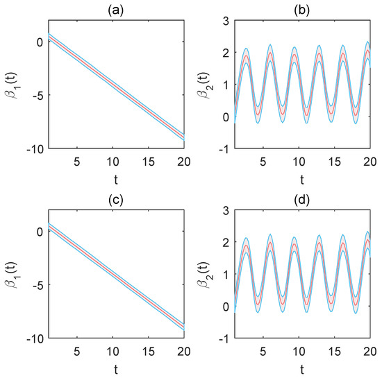
Figure 1.
Confidence intervals of and in Example 1 at and with Gaussian errors. (a,b) The varying coefficients are approximated via the B-spline basis. (c,d) The varying coefficients are approximated via the local polynomial fitting scheme. The areas represent 95% point-wise confidence intervals.
Figure 2 shows that the estimated surface based on the B-spline surface fitting method is close to the true surface. The estimated surface based on local linear approximation is a plane. Thus, the B-spline surface fitting method is superior to the local linear approximation method.
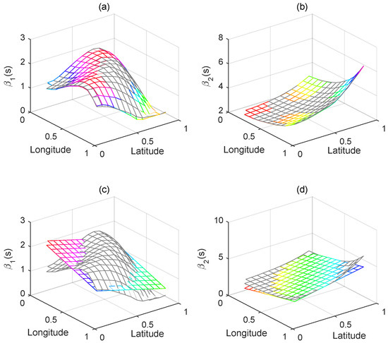
Figure 2.
The estimated and (multicolored surface) superimposed with the true and (grey surface) in Example 2 at and with Gaussian errors. (a,b) The varying coefficients are approximated via the B-spline surface fitting method. (c,d) The varying coefficients are approximated via local linear approximation.
6. Illustration
Economic development is an important research area in economics. The data used in this paper were collected from 31 provinces in China from 2005–2019 and can be obtained from the EPSDATA Databases (https://www.epsnet.com.cn/index.html#/Index, accessed on 12 March 2023). The dependent variable is the economic development level. Our analysis aims to model the effects of the industrial structure (IS), urbanization (Urban), openness (Open), higher education (Edu), and infrastructure (Infra) on different quantiles of the economic development level (GDP). The detailed variable definitions are presented in Table 5.
Table 5.
Variable definitions and descriptions.
6.1. Time-Varying Effects of the Covariates
Firstly, we try to find which covariates have time-varying effects on economic development and which covariates do not. We consider a set of quantiles with . At each quantile , the SIC criterion is applied for model selection. The results are summarized in Table 6. The obtained result shows the coefficients of Edu () and Infra () are constant, and the covariates IS (), Urban (), and Openness () have time-varying effects on the economic development. Additionally, the following QR model is considered:
where , is the -th element of , and is the spatial weight matrix generated by the longitude and latitude of the 31 regions [36]. We employ the B-spline curve fitting scheme to approximate the varying coefficients , , and .
Table 6.
SIC values and corresponding models. Only the first five smallest SIC values in descending order are listed, where represents all the covariates that have time-varying effects, ∅ represents all the constant coefficients, and stands for , ⋯, and indicates which models have time-varying effects.
The MLE and bias-corrected FEQR estimates of , , and at quantiles are reported in the top half of Table 7. The results show that the spatial correlation coefficient is positive, which means that the economic growth rates in a neighborhood affect each other and the impact is positive. Additionally, Edu () and Infra () positively affect economic development at quantiles .
Table 7.
Estimates of , and at quantiles .
Figure 3a–c plot the surfaces of the estimated , , and . The x-axis represents the years, the y-axis represents the quantiles, and the z-axis represents the varying coefficients’ estimations. Figure 3 indicates that , , and all vary over time. The impact of industry structure (IS) is generally negative and gradually declines over time. The effect of urbanization (Urban) is positive and increases first then decreases. The impact of openness (Open) is initially negative and gradually becomes positive as time goes on.
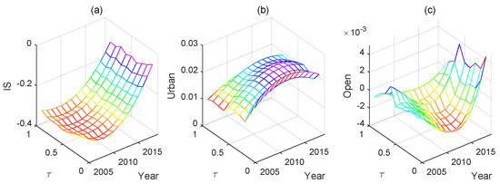
Figure 3.
The estimated surfaces of (a) , (b) , and (c) .
6.2. Location-Varying Effects of the Covariates
Following, we investigate the location effects of the impacts of the covariates and try to find which covariates have location-varying effects on the urban–rural income gap and which covariates do not. We consider a set of quantiles with . At each quantile , the SIC criterion is applied for model selection. The results are summarized in Table 8. The obtained results shows the effects of Edu () and Infra () are constant, and the coefficients of the rest of the covariates all have location-varying effects on the economic development level. The QR model is given by:
where . The B-spline surface fitting scheme is employed to approximate the varying coefficients , , and .
Table 8.
SIC values and corresponding models. Only the first five smallest SIC values in descending order are listed, where represents all the covariates that have location-varying effects, ∅ represents the coefficient of all the covariates that are constant, and stands for , ⋯, and indicates coefficients that have varying location effect.
The MLE and bias-corrected FEQR estimates of , , and at quantiles are reported in the latter part of Table 7, which shows that the spatial correlation coefficient is positive, which means that the economic development levels in a neighborhood affect each other and the impact is positive. Additionally, Edu () and Infra () positively affect economic development at quantiles .
Figure 4a–c plot the surface of the estimated , , and at quantile . The x-axis represents the latitude, the y-axis represents the longitude, and the z-axis represents the estimation of the varying coefficients. Figure 4a shows that the effect of industry structure (IS) is positive in low latitudes and gradually transforms to negative as the latitude increases. In general, the industry structure (IS) effect is more significant in Eastern China. Figure 4b indicates that the impact of openness (Open) is generally negative and gradually transforms to positive as the latitude increases. Figure 4c shows that openness (Open) generally hurts economic development and the negative impact becomes weaker as longitude and latitude increase.
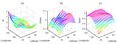
Figure 4.
The estimated surfaces of (a) , (b) , and (c) at .
7. Conclusions
This paper investigates a spatial quantile panel data model with varying coefficients. Both the time and location effects of the impacts of the covariates are taken into account, which allows us to investigate how the effects of covariates vary over time and location. The B-spline curve fitting scheme and the local polynomial approximation are employed to approximate the varying coefficient for the time-varying coefficient model. For the location-varying coefficient model, the local linear approximation is used for estimation since performing higher-order Taylor expansions on binary functions is difficult. Considering that the local linear estimator is too rough, the B-spline surface fitting method is introduced for approximation.
Moreover, the FEQR estimation is biased in the presence of the spatial lag variable. Thus, the wild bootstrap method is employed for bias correction. The proposed model relaxes the homogeneous slope assumption and can accommodate heterogeneity in the regression function and thus balances better between model flexibility and parsimony. Further, the estimation approach relaxes the normality assumption and therefore does not require any specification of the error distribution.
Important and interesting further studies can be conducted by considering three-dimensional spatiotemporal-varying coefficients. This paper applies the SIC criterion for model structure identification, i.e., identification of varying and constant coefficients. In future work, we hope to propose a penalty method to simultaneously achieve parameter estimation, variable selection, and model structure identification, which is more convenient and efficient in practical applications.
Author Contributions
Conceptualization, X.D., L.J. and M.T.; Methodology, X.D.; Investigation, X.D.; Simulation studies, X.D., S.H. and L.J.; Visualization, X.D.; Formal analysis, X.D.; Funding acquisition, L.J.; Writing—original draft preparation, X.D.; Writing—review and editing, X.D., S.H., L.J. and M.T.; Project administration, X.D.; Supervision, L.J. and M.T. All authors have read and agreed to the published version of the manuscript.
Funding
The work was funded by the National Natural Science Foundation of China (No. 11801370).
Data Availability Statement
The economic development data can be obtained from the EPSDATA Databases. https://www.epsnet.com.cn/index.html#/Index (accessed on 12 March 2023).
Conflicts of Interest
The authors declare no conflict of interest.
References
- Anselin, L.; Sheri, H. Spatial econometrics in practice, a review of software options. Reg. Sci. Urban Econ. 1992, 22, 509–536. [Google Scholar] [CrossRef]
- Anselin, L. Spatial econometrics. In A Companion to Theoretical Econometrics; Baltagi, B.H., Ed.; Blackwell Publishing Ltd.: Malden, MA, USA, 2003; pp. 310–330. [Google Scholar]
- Baltagi, B.; Song, S.H.; Koh, W. Testing panel data regression models with spatial error correlation. J. Econom. 2003, 117, 123–150. [Google Scholar] [CrossRef]
- Baltagi, B.H.; Song, S.; Jung, B.; Koh, W. Testing for serial correlation, spatial autocorrelation and random effects using panel data. J. Econom. 2007, 140, 5–51. [Google Scholar] [CrossRef]
- Baltagi, B.H.; Kao, C.; Liu, L. Asymptotic properties of estimators for the linear panel regression model with random individual effects and serially correlated errors: The case of stationary and non-stationary regressors and residuals. J. Econom. 2008, 11, 554–572. [Google Scholar] [CrossRef]
- Baltagi, B.; Egger, P.; Pfaffermayr, M. A generalized spatial panel data model with random effects. Econom. Rev. 2013, 32, 650–685. [Google Scholar] [CrossRef]
- Dai, X.; Yan, Z.; Tian, M.; Tang, M. Quantile regression for general spatial panel data models with fixed effects. J. Appl. Stat. 2020, 47, 45–60. [Google Scholar] [CrossRef]
- Elhorst, J. Paul Dynamic models in space and time. Geogr. Anal. 2001, 33, 119–140. [Google Scholar] [CrossRef]
- Elhorst, J.P. Specification and estimation of spatial panel data models. Int. Reg. Sci. Rev. 2003, 26, 244–268. [Google Scholar] [CrossRef]
- Elhorst, J.P. Unconditional maximum likelihood estimation of linear and log-linear dynamic models for spatial panels. Geogr. Anal. 2005, 37, 85–106. [Google Scholar] [CrossRef]
- Kapoor, M.; Kelejian, H.H.; Prucha, I.R. Panel data models with spatially correlated error components. J. Econom. 2007, 140, 97–130. [Google Scholar] [CrossRef]
- Lee, L.F.; Yu, J.H. Estimation of spatial autoregressive panel data models with fixed effects. J. Econom. 2010, 154, 165–185. [Google Scholar] [CrossRef]
- Yu, J.; de Jong, R.; Lee, L.F. Quasi-maximum likelihood estimators for spatial dynamic panel data with fixed effects when both n and T are large. J. Econom. 2008, 146, 118–134. [Google Scholar] [CrossRef]
- Yu, J.; Lee, L.F. Estimation of unit root spatial dynamic panel data models. Econom. Theory 2010, 26, 1332–1362. [Google Scholar] [CrossRef]
- Michael, O.; Robert, P.B. Spatial analysis of municipal water demand: A panel data approach. Appl. Econ. Lett. 2018, 25, 1157–1160. [Google Scholar]
- Guliyev, H. Determining the spatial effects of covid-19 using the spatial panel data model. Spat. Stat. 2020, 38, 100443. [Google Scholar] [CrossRef] [PubMed]
- Huang, N.; Yang, Z. Spatial dynamic models with short panels: Evaluating the impact of purchase restrictions on housing prices. Econ. Model. 2021, 103, 105597. [Google Scholar] [CrossRef]
- Yang, C.F. Common factors and spatial dependence: An application to US house prices. Econom. Rev. 2021, 40, 14–50. [Google Scholar] [CrossRef]
- Lee, K.; Pesaran, M.H.; Smith, R. Growth and convergence in a multi-country empirical stochastic Solow model. J. Appl. Econom. 1997, 12, 357–392. [Google Scholar] [CrossRef]
- Brunsdon, C.; Fotheringham, S.; Charlton, M. Geographically Weighted Regression. J. R. Stat. Soc. Ser. D (Stat.) 1998, 47, 431–443. [Google Scholar] [CrossRef]
- Zhang, Y.; Shen, D. Estimation of semi-parametric varying-coefficient spatial panel models with random-effects. J. Stat. Plan. Inferences 2015, 159, 64–80. [Google Scholar] [CrossRef]
- Sun, Y.; Malikov, E. Estimation and inference in functional-coefficient spatial autoregressive panel data models with fixed effects. J. Econom. 2018, 203, 359–378. [Google Scholar] [CrossRef]
- Mínguez, R.; Basile, R.; Durbán, M. An alternative semiparametric model for spatial panel data. Stat. Methods Appl. 2020, 29, 669–708. [Google Scholar] [CrossRef]
- Dai, X.; Jin, L.; Shi, A.; Shi, L. Outlier Detection and Accommodation in General Spatial Models. Stat. Methods Appl. 2016, 25, 453–475. [Google Scholar] [CrossRef]
- Dai, X.; Li, S.; Jin, L.; Tian, M. Quantile regression for partially linear varying coefficient spatial autoregressive models. Commun. Stat. Simul. Comput. 2022. [Google Scholar] [CrossRef]
- Dai, X.; Jin, L. Minimum distance quantile regression for spatial autoregressive panel data models with fixed effects. PLoS ONE 2021, 16, e0261144. [Google Scholar] [CrossRef] [PubMed]
- Xu, X.; Lee, L.F. A spatial autoregressive model with a nonlinear transformation of the dependent variable. J. Econom. 2015, 186, 209–232. [Google Scholar] [CrossRef]
- Feng, X.; He, X.; Hu, J. Wild bootstrap for quantile regression. Biometrika 2011, 98, 995–999. [Google Scholar] [CrossRef]
- Wang, L.; Keilegom, I.; Maidman, A. Wild residual bootstrap inference for penalized quantile regression with heteroscedastic errors. Biometrika 2018, 105, 859–872. [Google Scholar] [CrossRef]
- Kim, M.O. Quantile regression with varying coefficients. Ann. Stat. 2007, 35, 92–108. [Google Scholar] [CrossRef]
- Lu, Y.Q. Estimation for the Power-transformed Varying-coefficient Quantile Regression Model. Commun. Stat. Theory Methods 2013, 42, 2617–2633. [Google Scholar] [CrossRef]
- Wang, H.X.; Zhu, Z.Y.; Zhou, J.H. Quantile regression in partially linear varying coefficient models. Ann. Statist. 2009, 37, 3841–3866. [Google Scholar] [CrossRef]
- Galvao, A.F.; Montes-Rojas, G. On Bootstrap Inference for Quantile Regression Panel Data: A Monte Carlo Study. Econometrics 2015, 3, 654–666. [Google Scholar] [CrossRef]
- Sun, Y.; Yan, H.J.; Zhang, W.Y.; Lu, Z.D. A Semiparametric Spatial dynamic model. Ann. Stat. 2014, 42, 700–727. [Google Scholar] [CrossRef]
- Elhorst, J.P. Spatial Panal Data Models. In Handbook of Applied Spatial Analysis; Fischer, M.M., Getis, A., Eds.; Springer: Berlin/Heidelberg, Germany; New York, NY, USA, 2010; pp. 377–407. [Google Scholar]
- LeSage, J.P. The Theory and Practice of Spatial Econometrics; University of Toledo: Toledo, OH, USA, 1999. [Google Scholar]


Disclaimer/Publisher’s Note: The statements, opinions and data contained in all publications are solely those of the individual author(s) and contributor(s) and not of MDPI and/or the editor(s). MDPI and/or the editor(s) disclaim responsibility for any injury to people or property resulting from any ideas, methods, instructions or products referred to in the content. |
© 2023 by the authors. Licensee MDPI, Basel, Switzerland. This article is an open access article distributed under the terms and conditions of the Creative Commons Attribution (CC BY) license (https://creativecommons.org/licenses/by/4.0/).