Wave Scattering through Step Down Cascading Junctions

Abstract

In this paper, we present the scattering of plane waves through two junctions with step-down cascading discontinuities. The solutions in the form of trapped modes corresponding to discrete eigen values are also presented. We illustrate the matching of continuity of pressure and velocity at the edges, conservation of energy, convergence/error of reflection, and reflection and transmission of the incident wave that go through the wider region. We discuss the reflection and transmission amplitudes by varying dimensions of wave-guide structure against wave number. We plot the surface and contour plots along with absolute potential solutions at different frequencies where extrema of field amplitudes occur. We also derive the results of extra ordinary acoustic transmission (EAT) for existing models. We apply the Mode Matching Method (MMM) to tackle the problem. Our model would be beneficial to structure the old and new models containing cavities and junctions. However, these structure models cannot retrieve our proposed geometrical model. The results will be helpful to model the practical exhaust system in noise reduction theory.

1. Introduction

Wave-guide through cascaded-up or cascaded-down discontinuities plays a significant role in mechanical engineering for the designing of networks and integrated circuits at optical and exhaust models for numerous devices to minimize sound and improve their performance; therefore, wave scattering through cascade discontinuities in junctions is especially important. We have practiced MMM in our cascaded-down junction problem. The geometry is such that the two infinite parallel rods are twisted at two horizontal points $-l_2$ and $-l_1$ providing two vertical barriers that are points of discontinuities.

MMM is a useful method for boundary-value problems, especially for geometries consisting of two or more separate regions. It is based on matching the solutions in terms of eigen functions expansions at the boundaries of the different regions, as discussed in chapter 2 of ref. [1]. In ref. [2] MMM is applied to three different resonators, using symmetry and without symmetry. The conclusion was drawn that if there is no symmetry, then extraordinary acoustic transmission cannot be obtained generally and symmetry plays a critical role in extraordinary transmission. In ref. [3], the Mode Matching Method is applied for the analysis of cascaded discontinuities in a rectangular wave guide for computing the transmission characteristics and voltage standing wave ratio (VSWR) of cascaded H-Plane discontinuity. They have also compared MMM with other numerical methods. Refs. [4,5] have provided the solution in the form of trapped modes in a cavity duct wave-guide containing outer cavities. In ref. [6], diffraction of a sound wave is analyzed in a semi-infinite cylinder with a cavity that contains partial lining. Wiener-Hopf (WH) equations are obtained for solutions. MMM and Fourier transformations are applied to obtain WH-equations. In ref. [7], wave scattering is analyzed in a semi-infinite rigid tube that is inserted into a large, lined tube of infinite length containing absorbent material. WH technique is applied. A rigorous Model Analysis (MA) is offered for the H-plane wave-guide T-junction loaded with a post structure. The analysis is presented on the classical resonator mode-matching scheme and introduces the concept of “extended eigen-mode functions” has been introduced. This concept can be applied to the computation of several complex canonical guided-wave problems along with MA [8]. Ref. [9] has constituted a three spaced wave-guide by symmetrically situating a duct inside an infinite duct, and MMM has been applied for soft and hard boundary conditions. The sound radiation in a planar trifurcated lined duct is tackled via MMM [10,11]. The scattering matrix approach and MMM are used for analyzing rectangular wave-guide H-plane junctions for electromagnetic research [12,13] and in a resonator circuit, including micro-wave circuits [14]. MMM for analyzing cascaded discontinuities is important in network design and noise reduction as the scientists are struggling to manufacture high-quality silencers to increase the lifetime of the mechanisms of several devices; therefore, we have worked on this problem with this context in mind. We show the effects of jump down discontinuities on field amplitudes in terms of the intensity of waves, destructive and constructive interferences. We have also shown how different predicted models can be generated from our considered geometry, which would be useful to model more practical exhaust models.

The outline of our work is as follows. In Section 2, we have considered the cascaded-down wave-guide for parallel plates having two vertical junctions. We have presented the schematic diagram along with the boundary conditions. In Section 3, we have divided our problem into three different regions and given general solutions. In Section 4, we have formulated an infinite system of equations using MMM, exploiting the continuity of pressure and velocity across the regions. In Section 5, we formulate the graphical results using MATLAB coding and draw the conclusions from the graphical results for existing and non-existing ducts. Section 6 is a summary of the research.

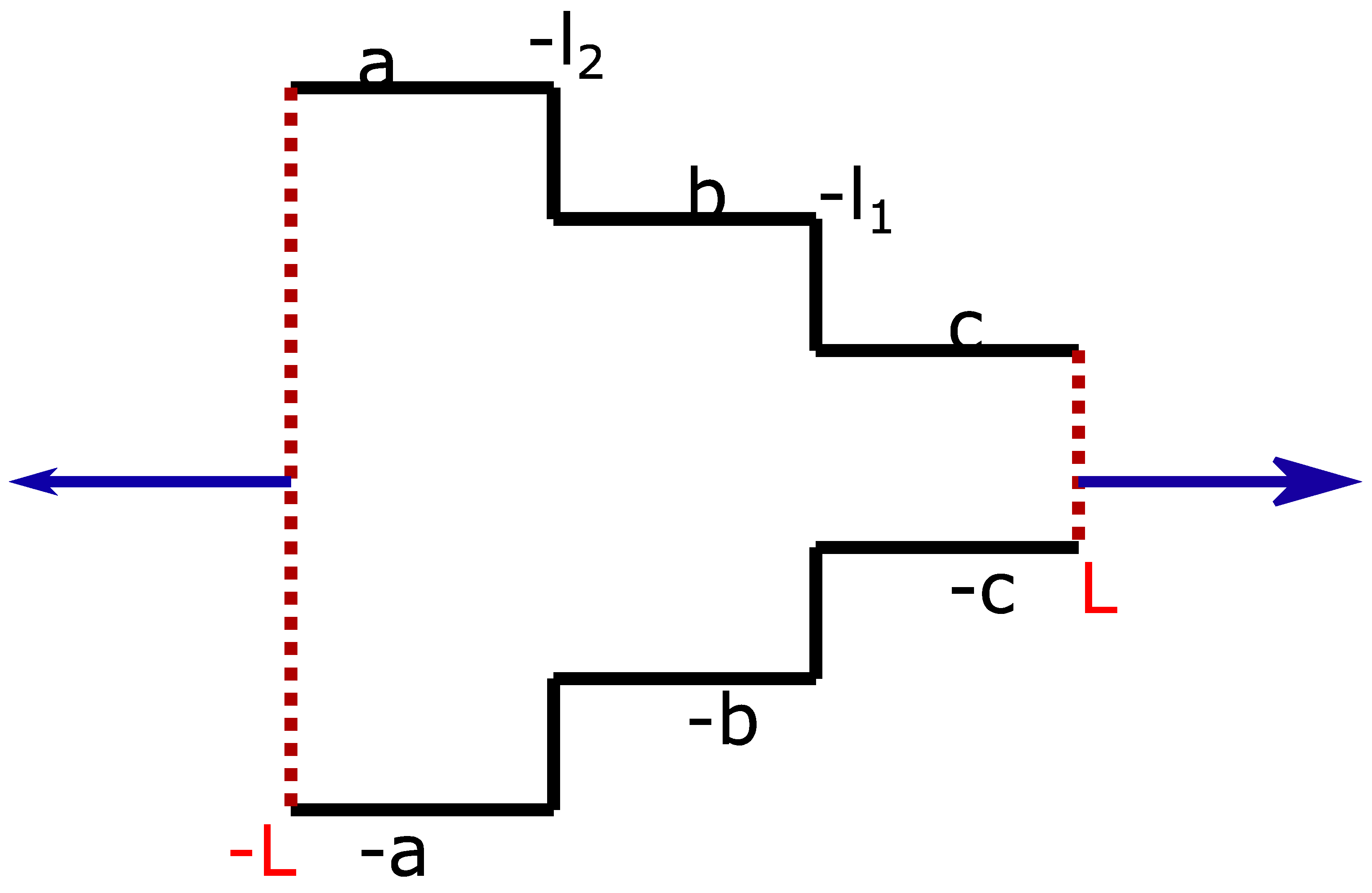
2. Geometry of Cascaded-Down Junctions

We initiate our work by taking the general of two-dimensional wave equation i.e., $\frac{{\partial }^2\Phi }{\partial x^2}+\frac{{\partial }^2\Phi }{\partial y^2}=\frac{1}{c_2}\frac{{\partial }^2\Phi }{\partial t^2}$. We familiarize scalar potential function $\Phi (x,y,t)=Re\left[\varphi (x,y)e^{-i\omega t}\right]$ which provides us two dimensional Helmholtz equation, ${\nabla }^2\varphi (x,y)+k^2\varphi (x,y)=0$ and k is defined as $k={\displaystyle \frac{\omega }{v}}$ where $\omega$ is angular frequency, v is speed of sound, and k shows wave number. ${\nabla }^2$ is the Laplacian operator. We define pressure by $p=-{\rho }_0{\displaystyle \frac{\partial \Phi }{\partial t}}$ and the velocity vector by $\mathbf{u}=grad(\Phi )$ and ${\rho }_0$ represents the density of equilibrium state. The geometry of two cascaded down junctions is as displayed in Figure 1.

We will compute the results from leading Helmholtz Equation (1) subject to the following hard boundary conditions:

$${\nabla }^2\varphi (x,y)+k^2\varphi (x,y)=0$$

(1)

• ${\varphi }_y=0,y=\pm a,-\infty <x<-l_2$
• ${\varphi }_y=0,y=\pm b,-l_2<x<-l_1$
• ${\varphi }_y=0,y=\pm c,-l_1<x<\infty$
• ${\varphi }_x=0,x=-l_2,-a<y<-b,b<y<a$
• ${\varphi }_x=0,x=-l_1,-b<y<-c,c<y<b$
  In addition, radiation conditions would also be applied. We divide this infinite duct into three regions as discussed below.

3. Solution of Regions Separately

3.1. Region 1: $(-\infty <x\le -l_2,-a\le y\le a)$

The above discussion and geometry clarifies that we have two hard boundary conditions at verticals in this region, i.e., ${\varphi }_y(x,a)=0$ and ${\varphi }_y(x,-a)=0$. We apply separation of variables and attain the solution as Equation (2). From this result, we will develop Mode Matching Technique after computing the solutions of Region 2 and Region 3.

$${\varphi }_1(x,y)=\sum _{n=0}^{\infty }{A}_n{e}^{-i{\widehat{\alpha }}_n(x+l_2)}{\psi }_n(y)+e^{i\widehat{{\alpha }_0}(x+l_2)}{\psi }_0(y)$$

(2)

where ${\alpha }_n=\frac{n\pi }{2a}$, and ${\widehat{\alpha }}_n=\sqrt{k^2-{\alpha }_n^2}$. The coefficients $A_n$ represent reflected field amplitudes and $e^{i\widehat{{\alpha }_0}(x+l_2)}{\psi }_0(y)$ represents the incident wave which propagates from left to right.

$${\psi }_n(y)=\left\{\begin{array}{cc}\sqrt{\frac{1}{a}}cos{\alpha }_n(y-a),\hfill & n\ne 0,\\ \sqrt{\frac{1}{2a}},\hfill & n=0,\end{array}\right.$$

which are orthonormal i.e., ${\int }_{-a}^a{\psi }_m(y){\psi }_n(y)dy={\delta }_{mn}$, where

$${\delta }_{mn}=\left\{\begin{array}{cc}0,\hfill & m\ne n,\hfill \\ 1,\hfill & m=n.\hfill \end{array}\right.(\ast )$$

3.2. Region 2: $(-l_2\le x\le -l_1,-b\le y\le b)$

We notice from geometry that horizontal limits are finite and hard boundary conditions at verticals are ${\varphi }_y(x,b)=0$ and ${\varphi }_y(x,-b)=0$. In Region 2 solution is defined as Equation (3).

$${\varphi }_2(x,y)=\sum _{n=0}^{\infty }(C_n{e}^{i{\widehat{\beta }}_n(x+l_2)}+D_n{e}^{-i{\widehat{\beta }}_n(x+l_1)}){\xi }_n(y)$$

(3)

$C_n$ and $D_n$ correspond to the coefficients of wave propagating to the right and left respectively. Where ${\beta }_n=\frac{n\pi }{2b}$ and ${\widehat{\beta }}_n=\sqrt{k^2-{\beta }_n^2}$. The vertical eigen functions are computed as.

$${\xi }_n(y)=\left\{\begin{array}{cc}\sqrt{\frac{1}{b}}cos{\beta }_n(y-b),\hfill & n\ne 0,\hfill \\ \sqrt{\frac{1}{2b}}\hfill & n=0,\hfill \end{array}\right.$$

which are orthonormal as ${\int }_{-b}^b{\xi }_m(y){\xi }_n(y)dy={\delta }_{mn}$.

3.3. Region 3: $(-l_1\le x<\infty ,-c\le y\le c)$

Associated boundary conditions at verticals are ${\varphi }_y(x,\pm c)=0$ and general solution in this region is computed as in Equation (4).

$${\varphi }_3(x,y)=\sum _{n=0}^{\infty }(B_n{e}^{i{\widehat{\gamma }}_n(x+l_1)}){\eta }_n(y)$$

(4)

where as ${\gamma }_n=\frac{n\pi }{2c}$ and ${\widehat{\gamma }}_n=\sqrt{k^2-{\gamma }_n^2}$. Here the coefficients $B_n$ represent the transmitted field amplitudes and eigen functions are

$${\eta }_n(y)=\left\{\begin{array}{cc}\sqrt{\frac{1}{c}}cos{\gamma }_n(y-c),\hfill & n\ne 0,\hfill \\ \sqrt{\frac{1}{2c}},\hfill & n=0,\hfill \end{array}\right.$$

which are orthonormal. The radiation conditions are also applied in region, 1 and 3. Note that $a\ne 0,b\ne 0$ and $c\ne 0$. In Figure 2, the column on the left hand side shows real, imaginary, and absolute surface plots of the potential functions, and the right column shows contour plots, respectively, for $a=3,b=2,c=1,k=1$. The potential functions correspond to as $-5\le x\le -2$, $-3\le y\le 3$ for region I, $-2\le x\le -1$, $-2\le y\le 2$ for region II and $-1\le x\le 5$, $-1\le y\le 1$ for region III. The surface plots relate to the two continuous variables x and y, while the contour plots relate to the 2-dimensional view. In real parts intensity of wave is maximum in the middle near $x=-2,-1$, $x=0$ and $x=5$ and it reduces on either side of it. In imaginary parts intensity is less near $x=-2,-1$ in the middle and it increases on either side. While it is large near $x=0,5$ in middle along $x$-axis and it reduces on either side. In absolute terms, intensity is large at $y=0$ and it reduces on either side near $x=-2,-1$, $x=0$ and $x=5$.

4. Formulation of System of Equations

In this section, we derive a system of equations which arise from the mode matching technique.

4.1. Continuity of Pressures

Continuity of pressure across $x=-l_2$ gives

$$\sum _{n=0}^{\infty }{A}_n{\psi }_n(y)+{\psi }_0(y)=\sum _{n=0}^{\infty }(C_n+D_n{e}^{-i{\widehat{\beta }}_n(l_1-l_2}){\xi }_n(y)$$

(5)

taking inner product with ${\xi }_m(y)$ and integrating over $[-b,b]$ using orthonormality conditions we get

$$\sum _{n=0}^{\infty }{A}_n{l}_{mn}+l_{m0}=C_m+D_m{e}^{-i{\widehat{\beta }}_m(l_1-l_2})m=0,1,2,\dots$$

(6)

and $l_{mn}={\int }_{-b}^b{\psi }_n(y){\xi }_m(y)dy$ are calculated as below.

$$l_{mn}=\left\{\begin{array}{cc}0\hfill & n=0,m\ne 0\hfill \\ \sqrt{\frac{1}{2ab}}\frac{1}{{\alpha }_n}[sin{\alpha }_n(b-a)+sin{\alpha }_n(a+b)]\hfill & m=0,n\ne 0\hfill \\ \frac{1}{\sqrt{16ab}{\beta }_m}[sin{\beta }_m(b-a)+sin{\beta }_m(3a+b)+4b{\beta }_{m}cos{\beta }_m(b-a)]\hfill & {\alpha }_n={\beta }_m\hfill \\ \frac{1}{\sqrt{ab}}[{\alpha }_{n}sin{\alpha }_n(b-a)+{\alpha }_{n}sin{\alpha }_n(a+b)cos{\beta }_m(2b)]\frac{1}{({\alpha }_n^2-{\beta }_m^2)}\hfill & othercases\hfill \end{array}\right.$$

The continuity of pressure across $x=-l_1$ gives

$$\sum _{n=0}^{\infty }[C_n{e}^{i{\widehat{\beta }}_n(-l_1+l_2)}+D_n]{\xi }_n(y)=\sum _{n=0}^{\infty }{B}_n{\eta }_n(y)$$

(7)

taking inner product with ${\eta }_m(y)$ and integrating over $[-c,c]$ we get

$$\sum _{n=0}^{\infty }[C_n{e}^{i{\widehat{\beta }}_n(l_2-l_1)}+D_n]p_{mn}=B_{m}m=0,1,2,\dots$$

(8)

and $p_{mn}$ are calculated as below:

$$p_{mn}=\left\{\begin{array}{cc}\sqrt{\frac{c}{b}}\hfill & m=0,n=0\hfill \\ 0\hfill & n=0,m\ne 0\hfill \\ \sqrt{\frac{1}{2bc}}\frac{1}{{\beta }_n}[sin{\beta }_n(c-b)+sin{\beta }_n(b+c)]\hfill & m=0,n\ne 0\hfill \\ \frac{1}{\sqrt{16bc}{\gamma }_m}[sin{\gamma }_m(c-b)+sin{\gamma }_m(3c+b)+4c{\gamma }_{m}cos{\gamma }_m(c-b)]\hfill & {\beta }_n={\gamma }_m\hfill \\ \frac{1}{\sqrt{bc}}[{\beta }_{n}sin{\beta }_n(c-b)+{\beta }_{n}sin{\beta }_n(b+c)cos{\gamma }_m(2c)]\frac{1}{({\beta }_n^2-{\gamma }_m^2)}\hfill & othercases\hfill \end{array}\right.$$

4.2. Continuity of the Velocities of the Potential

The continuity of Velocity Potential across $x=-l_2$ gives

$$-\sum _{n=0}^{\infty }{A}_{n}i\widehat{{\alpha }_n}{\psi }_{n}y+{\psi }_0(y)i\widehat{{\alpha }_0}=\left\{\begin{array}{cc}0\hfill & -a\le y\le -b\hfill \\ \sum _{n=0}^{\infty }i{\widehat{\beta }}_n(C_n-D_n{e}^{-i{\widehat{\beta }}_n(-l_2+l_1)}){\xi }_n(y)\hfill & -b\le y\le c\hfill \\ 0\hfill & -c\le y\le c\hfill \end{array}\right.$$

Multiplying by ${\psi }_m(y)$ and integrating over $[-a,a]$ we obtain

$$i{A}_m\widehat{{\alpha }_m}+i\widehat{{\alpha }_0}{\delta }_{0m}=i\widehat{{\beta }_n}\sum _{n=0}^{\infty }(C_n-D_n{e}^{-i{\widehat{\beta }}_n(-l_2+l_1)})l_{nm}m=0,1,2,\dots$$

(9)

The continuity of velocity potential across $x=-l_1$, gives

$$i\widehat{{\beta }_n}\sum _{n=0}^{\infty }[C_n{e}^{i\widehat{{\beta }_n}(-l_1+l_2)}-D_n]{\xi }_n(y)=\left\{\begin{array}{cc}0\hfill & -b\le y\le -c\hfill \\ \sum _{n=0}^{\infty }i\widehat{{\gamma }_n}{B}_n{\eta }_n(y)\hfill & -c\le y\le c\hfill \\ 0\hfill & c\le y\le b\hfill \end{array}\right.$$

Multiplying by ${\xi }_m(y)$ and integrating over $[-b,b]$ we obtain

$$[C_m{e}^{-i{\widehat{\beta }}_m(-l_1+l_2)}i\widehat{{\beta }_m}-D_{m}i\widehat{{\beta }_m}]=\sum _{n=0}^{\infty }{B}_{n}i\widehat{{\gamma }_n}{p}_{nm}m=0,1,2,\dots$$

(10)

We truncate the infinite system of equations to a finite number of modes for numerical solution. We take M modes for $x<-l_2$ and N modes for $x<-l_1$ and obtain the following system.

$$\sum _{n=0}^M{A}_n{l}_{mn}+l_{m0}=C_m+D_m{e}^{-i{\widehat{\beta }}_m(l_1-l_2)}m=0,1,2,\dots ,N.$$

(11)

$$i{A}_m\widehat{{\alpha }_m}+i\widehat{{\alpha }_0}{\delta }_{0m}=i\widehat{{\beta }_n}\sum _{n=0}^N(C_n-D_n{e}^{-i{\widehat{\beta }}_n(-l_2+l_1)})l_{nm}m=0,1,2,\dots ,M.$$

(12)

$$\sum _{n=0}^N[C_n{e}^{i{\widehat{\beta }}_n(l_2-l_1)}+D_n]p_{mn}=B_{m}m=0,1,2,\dots ,M.$$

(13)

$$[C_m{e}^{-i{\widehat{\beta }}_m(-l_1+l_2)}i\widehat{{\beta }_m}-D_{m}i\widehat{{\beta }_m}]=\sum _{n=0}^M{B}_{n}i\widehat{{\gamma }_n}{p}_{nm}m=0,1,2,\dots ,N.$$

(14)

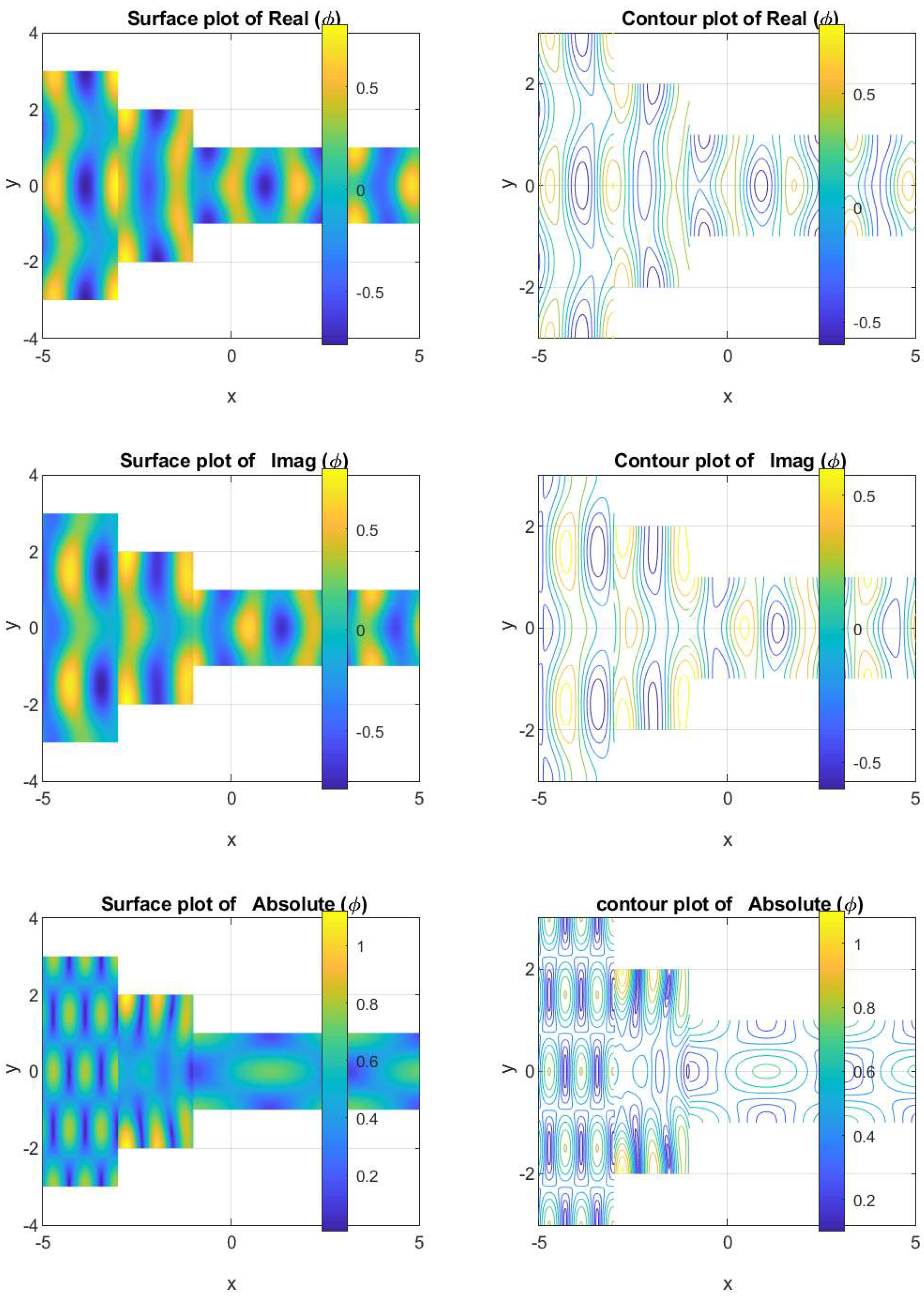
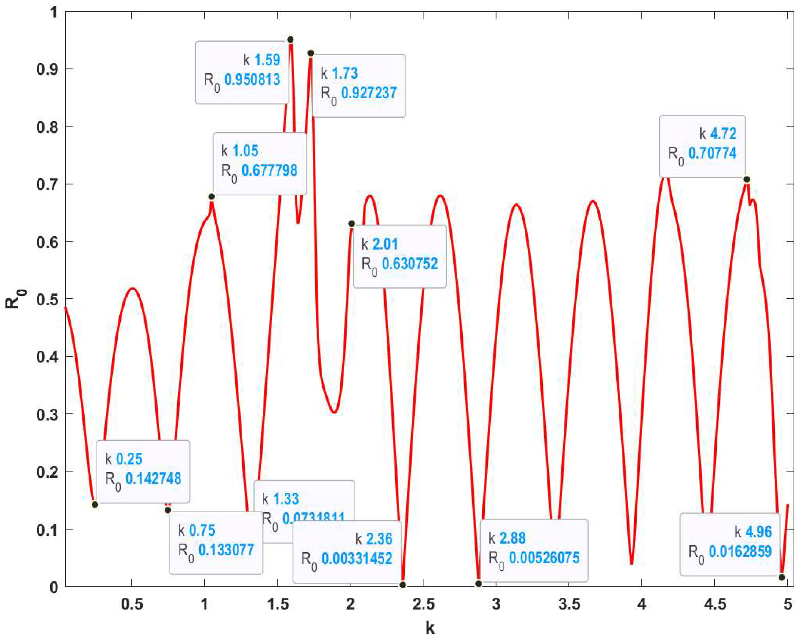
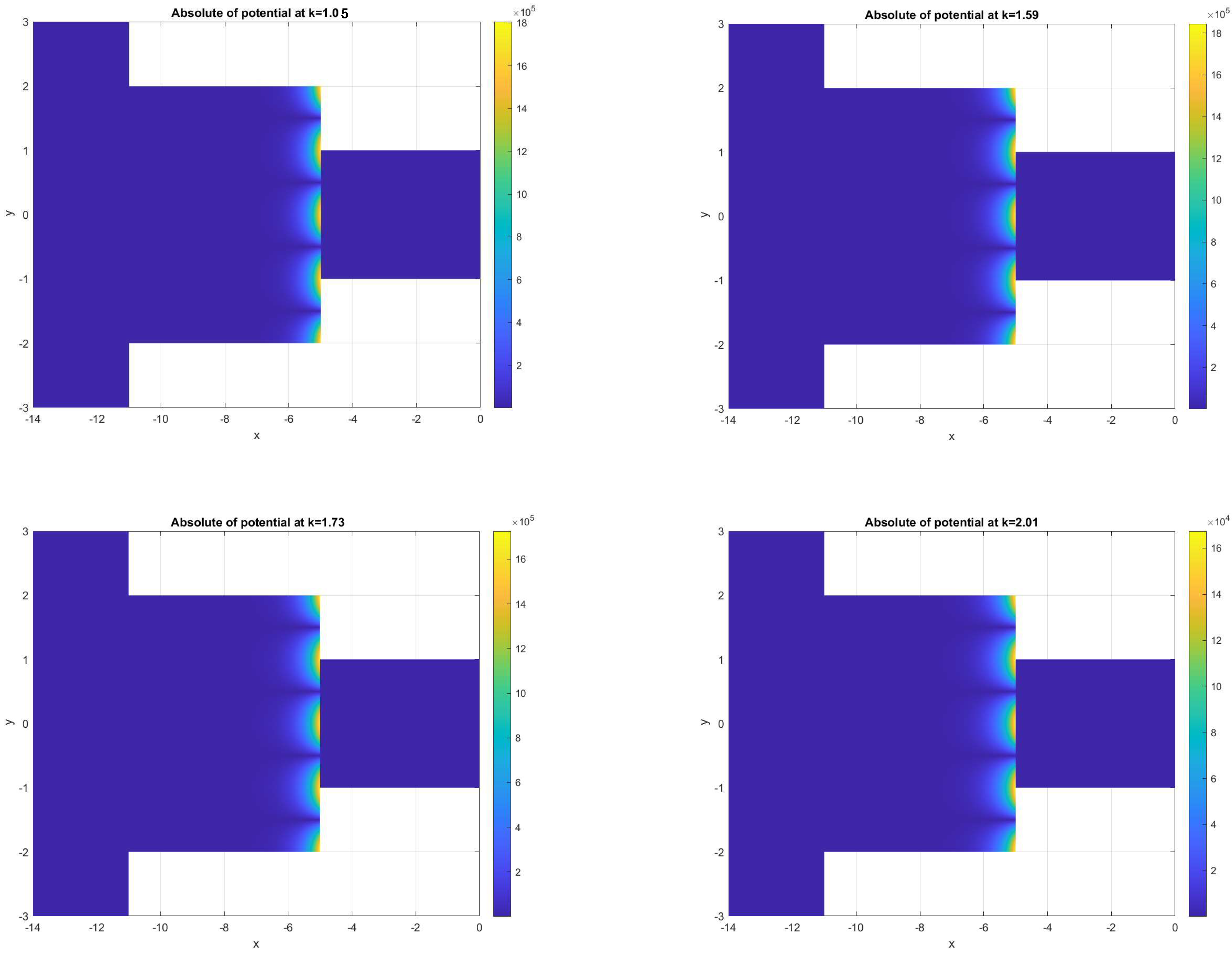
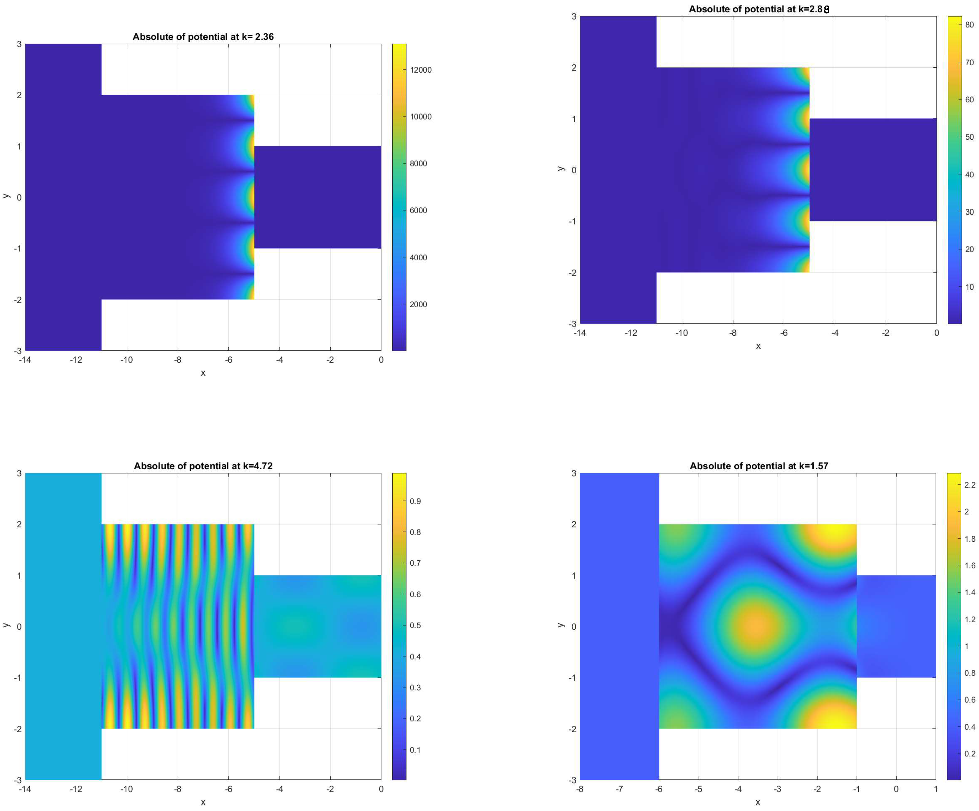
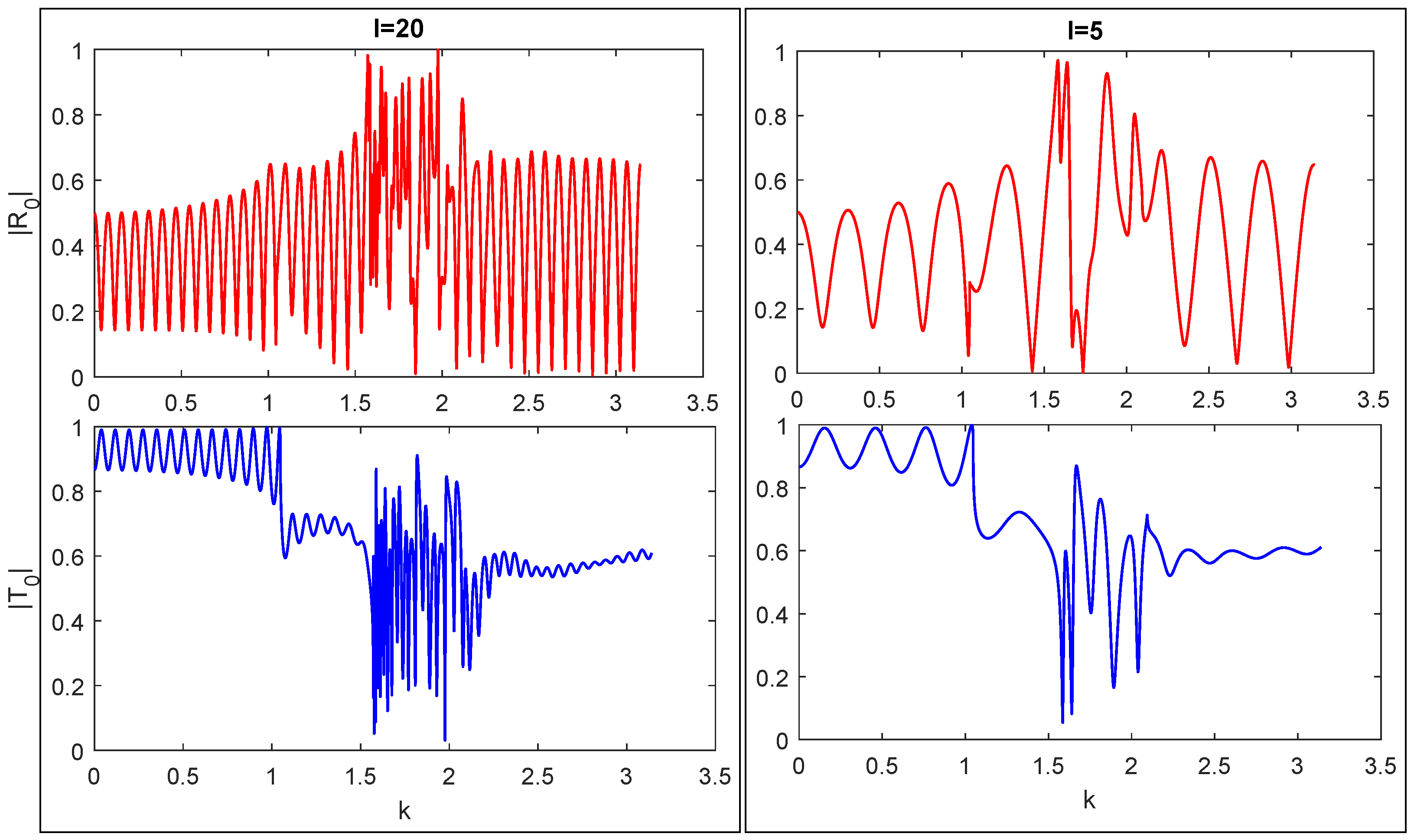
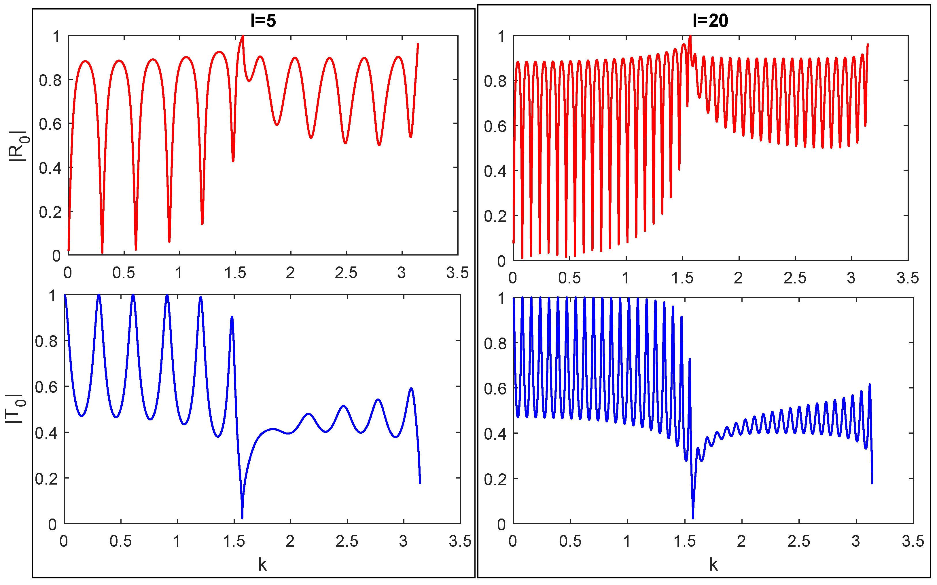
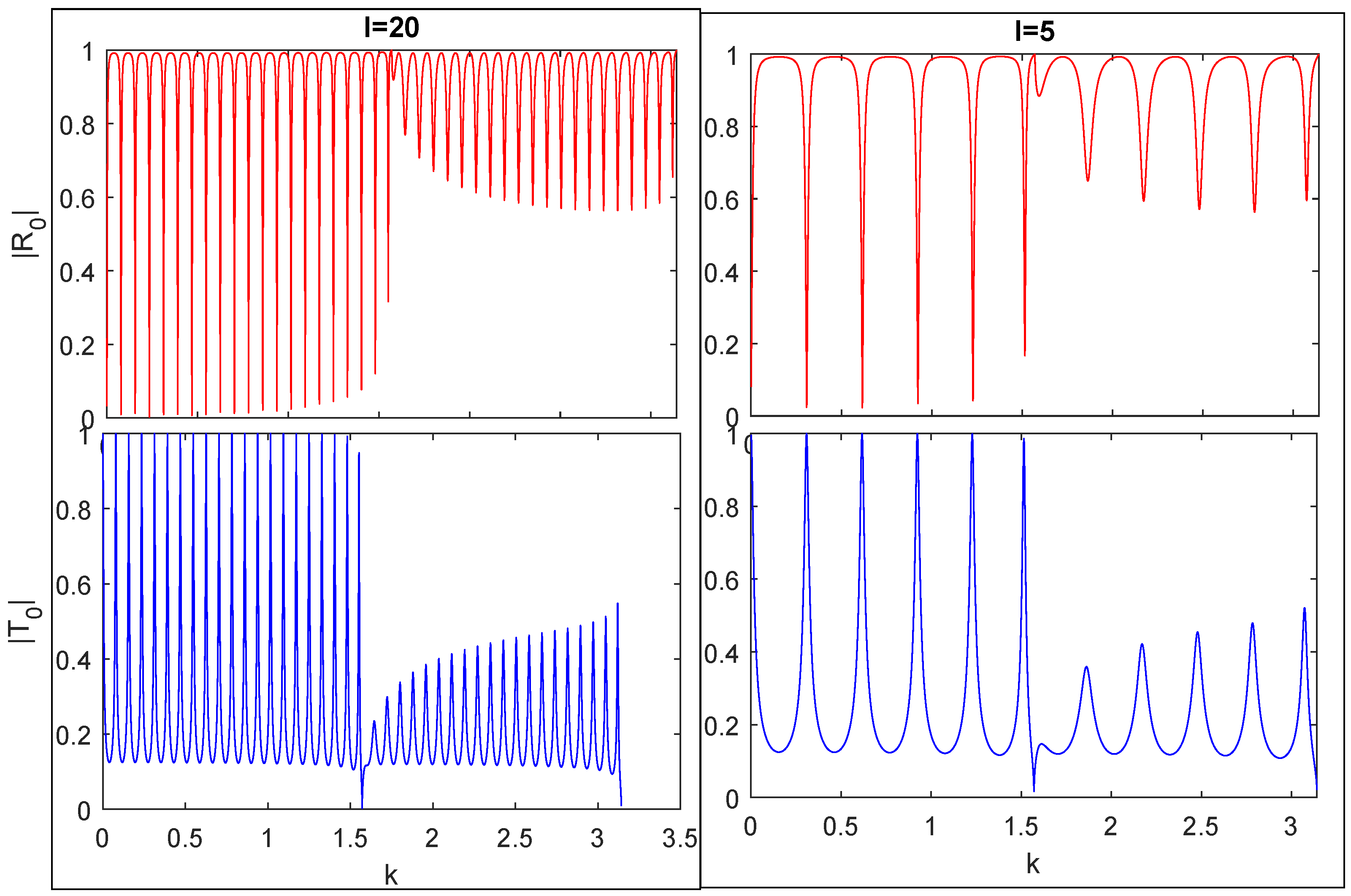
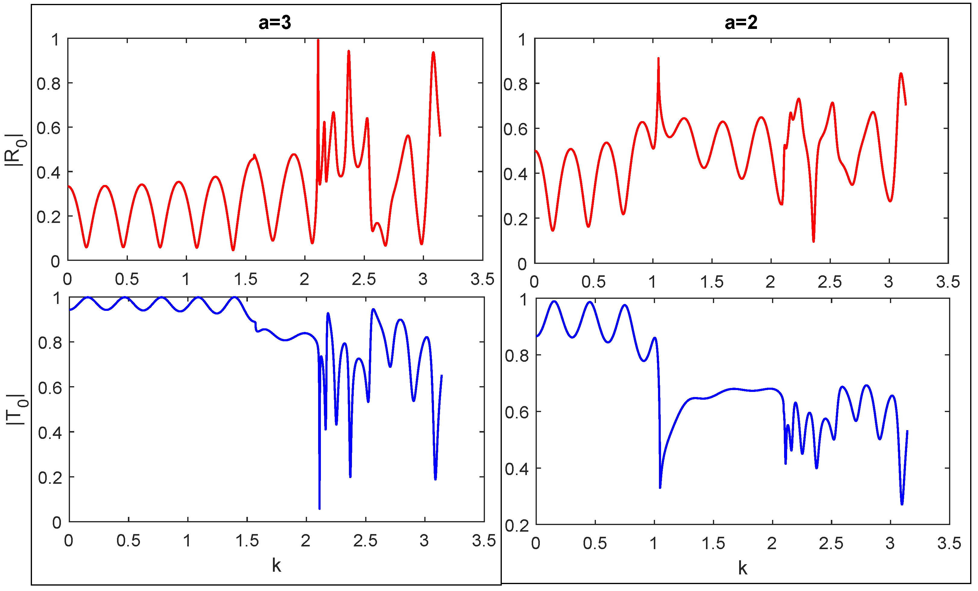
5. Graphical Results and Discussion

We have computed graphical results of matching at continuities, convergence/error, reflection, and transmission using MATLAB. We have introduced length l in some figures as $l=|l_2-l_1|$.

Figure 3 indicates continuity of velocity and pressure across two vertical interchanges $-l_2$ and $-l_1$. The top two graphs in Figure 3 are the matching of pressures across $-l_2$ and $-l_1$. We can observe that there is a perfect match as there is a tie in $({\varphi }_1,{\varphi }_2)$ versus the $|b|\le 2$ and $({\varphi }_2,{\varphi }_3)$ versus the $|c|\le 1$. The bottom two graphs of Figure 3 represent the matching for $({\varphi }_1^{{}^{\prime }},{\varphi }_2^{{}^{\prime }})$ versus $|b|\le 2$ and $({\varphi }_2^{{}^{\prime }},{\varphi }_3^{{}^{\prime }})$ versus $|c|\le 1$. Now we have calculated far-field reflection $R_0$ and transmission $T_0$. First of all, we see that either reflection and transmission converges, diverges, or oscillates by increasing the number of modes, as shown in the following Figure 4. The absolute value of the reflection coefficient $|R_0|$ versus the truncation number M and the absolute error are shown in Figure 4 where $l=4,a=1.5,b=1,c=0.5$ and $k=\pi /4$. In Figure 4B, we can see that the absolute error in the reflection coefficient turns in to zero. In Figure 4A, the absolute value $R_0$ becomes straight after $M\ge 20$, so we truncate the system of equations to twenty. Furthermore, we will examine wave scattering by computing the far-field reflection and transmission versus variation of k as in the following figures.

In Figure 5, we have computed the far-field reflection k against the wave number, which varies from 0 to 5. We can observe cut on/off frequencies at sharp edges, as indicated in figure. We will compute the potentials at the sharp edges to check whether we can obtain trapped modes or reflection-less modes.

In Figure 6, we computed the potential function $\varphi (x,y)$ at those values of k where the sharp edges of reflection coefficients can be seen in Figure 5. We have seen the trapped modes at discrete sets of eigen values.

In Figure 7, we have computed reflection and transmission for $a=3,b=2,c=1$ and $l=20,5$, $l=|l_2-l_1|$ here $|b-a|=|c-b|$ i.e., two junctions are of the same height. We notice more oscillations for $l=20$ as compared with $l=5$ of the given Figure 1.

One can also see that the reflection is minimum at some frequencies and the corresponding transmission is maximum up to $k\le \pi /3.$ Now we will see how the geometry of Figure 1 can be used for various types of ducts with cavities, as discussed in following Figure 8, Figure 9, Figure 10 and Figure 11 and so on.

As a special case, we take $a=c$ and $b<a$, results are plotted in Figure 8 and Figure 9. We have computed reflection and transmission for $a=2=c$, $b=0.5$ and $l=5,20$ in Figure 8 and for $a=2=c$, $b=0.125$ and $l=5,20$ in Figure 9. Furthermore, our cascaded duct of Figure 1 reduces to a duct with an inner cavity that is symmetric about both x-axis and y-axis. Our computed results in the above two figures closely match the results of ref. [2].

In Figure 10, we have taken values $a=0.5=c,b=2$ and $l=20,5$ then our two-junction, cascaded-down problem has just become a duct with an outer cavity. Our graphs represent the behavior of Extraordinary Acoustic Transmission (EAT) up to $k=\pi /2$ due to symmetries along both x-axis and y-axis (${\beta }_{2n}=\frac{n\pi }{b}$).

Figure 11 represents reflection and transmission by varying the width ‘a’ from $a=3$ to $a=2$ while the widths $b=1.5,c=1$ and the length $l=5$ are fixed. We see that the reflection amplitude is less for $a=3$ than for $a=2$, which agrees with the physical situation.

6. Conservation of Energy

We establish the energy conservation by Green’s second identity, i.e.,

$${\int \int \int }_{\Omega }(\varphi {\nabla }^2{\varphi }^{\ast }-{\varphi }^{\ast }{\nabla }^2\varphi )dv={\oint }_{\partial \Omega }({\varphi }^{\ast }\frac{\partial \varphi }{\partial n}-\varphi \frac{\partial {\varphi }^{\ast }}{\partial n})ds$$

(15)

${\varphi }^{\ast }$ is the complex conjugate of $\varphi$. Where $\varphi$ and ${\varphi }^{\ast }$ are continuous second order differentiable and n is outward normal to the surface, both $\varphi$ and ${\varphi }^{\ast }$ are the solutions of $({\nabla }^2+k^2)\varphi =0$ throughout the region, then the integrand with triple integral on L.H.S. of Equation (15) disappears identically, so the Equation (15) just remains as

$${\oint }_{\partial \Omega }({\varphi }^{\ast }\frac{\partial \varphi }{\partial n}-\varphi \frac{\partial {\varphi }^{\ast }}{\partial n})ds=0$$

(16)

In order to apply Green’s second identity. We need a closed region as $-\infty <x<\infty$ so we will take it as $-L<x<L$ as shown in Figure 12. Due to hard boundaries we have just two outward normals, as indicated by the arrows in Figure 11 that are along negative x direction and positive x direction.

Then Equation (15) becomes as follows.

$${\int }_{y=-a}^a(|-{\varphi }^{\ast }\frac{\partial {\varphi }_1}{\partial x}+\varphi \frac{\partial {\varphi }_1^{\ast }}{\partial x}{|}_{x=-L})dy+{\int }_{y=-c}^c(|{\varphi }^{\ast }\frac{\partial {\varphi }_3}{\partial x}-\varphi \frac{\partial {\varphi }_3^{\ast }}{\partial x}{|}_{z=L})dy=0$$

(17)

After substituting the required values and simplifying the equation of conservation energy balance, we get

$$\sum _{n=0}^{\infty }|A_n^2|Re(\widehat{{\alpha }_n})e^{iIm\widehat{{\alpha }_n}(-L+l_2)}-Re(\widehat{{\alpha }_0})e^{iIm\widehat{{\alpha }_0}(-L+l_2)}+\sum _{n=0}^{\infty }|B_n^2|e^{iIm\widehat{{\gamma }_n}(L+l_1)}Re\left[\widehat{n}\right]=0$$

(18)

In order to verify the equation we fix (18) as follows in (19).

$$\sum _{n=0}^N|A_n^2|Re(\widehat{{\alpha }_n})e^{iIm\widehat{{\alpha }_n}(-L+l_2)}-Re(\widehat{{\alpha }_0})e^{iIm\widehat{{\alpha }_0}(-L+l_2)}+\sum _{n=0}^N|B_n^2|e^{iIm\widehat{{\gamma }_n}(L+l_1)}Re\left[\widehat{{\alpha }_n}\right]=0$$

(19)

putting $N=0$ in (19) we get

$$|A_0^2|+|B_0^2|=1$$

(20)

Since ${\alpha }_n=n\pi /2a$, and $\widehat{{\alpha }_0}=\sqrt{k^2-{\alpha }_0^2}$ are purely real so its imaginary part becomes zero similarly ${\gamma }_n=n\pi /2c$, and $\widehat{{\gamma }_0}=\sqrt{k^2-{\gamma }_n^0}$ are purely real so its imaginary part becomes zero and Equation (20) gives:

$$|R_0^2|+|T_0^2|=1.$$

(21)

7. Summary

A detailed discussion for cascading-down junctions for the wave-guide problem is presented by applying Mode Matching Technique. Our geometrical model with two discontinuities is very important because it will be helpful for studying other diverse types of ducts and junction problems. We have computed the results regarding reflection and transmission of wave-guide structure by computing each case separately (Figure 5, Figure 7, Figure 8, Figure 9, Figure 10 and Figure 11). We have computed the solution at a discrete set of eigen values (Figure 5). We have observed that the modes can be trapped in cascading junctions. We have presented surface and contour plots (Figure 2), which help to predict dispersion, absorption, and probability density of a wave function. This can be revealed in the graphs of reflection and transmission. That is, for minimum transmission, reflection is large, and the probability of wave trapped in region 2. For dispersion, the reflection is minimum and the transmission is maximum. We have noticed constructive and destructive interferences at cut on/off frequencies (Figure 6), which would be beneficial to attenuate the unwanted noise. The results in (Figure 8) are matched with the work on extraordinary acoustic transmission [2]. The conservation law of the energy balance equation also holds. Our problem is the generalized case, as it would be helpful in designing further non-existing models that have applications in the field of noise-reduction for various kinds of silencing devices.

References

1. Linton, C.M.; McIver, P. Handbook of Mathematical Techniques for Wave/Structure Interactions; CRC Press LLC.: Boca Raton, FL, USA, 2001. [Google Scholar]
2. Meylan, M.H.; Ul Hassan, M.; Bashir, A. Extraordinary acoustic transmission, symmetry, blaschke products and resonators. Wave Motion 2017, 74, 105–123. [Google Scholar] [CrossRef]
3. Latha, C.; Payel, M. Mode matching method for the analysis of cascaded discontinuities in a rectangular Wave guide. Procedia Comput. Sci. 2016, 93, 251–258. [Google Scholar] [CrossRef]
4. Ma, C.; Niu, P.; An, X. The estimation of trapped modes in a cavity–duct wave-guide based on the coupling of acoustic and flow fields. Appl. Sci. 2023, 13, 1489. [Google Scholar] [CrossRef]
5. Dai, X. Total reflection of two guided waves for embedded trapped modes. AIAA 2020, 53, 131–139. [Google Scholar] [CrossRef]
6. Burhan, T. Sound wave diffraction by a cavity with partial lining. Math. Sci. Appl. 2020, 8, 123–133. [Google Scholar]
7. Rawlins, A.D. A bifurcated circular wave-guide problem. IMA J. Appl. Math. 1995, 54, 59–81. [Google Scholar] [CrossRef]
8. Wu, K.L.; Wang, H. A rigorous modal analysis of H-plane wave guide T-junction loaded with a partial-height post for wide-band applications. IEEE Trans. Microw. Theory Tech. 2001, 49, 893–901. [Google Scholar] [CrossRef]
9. Ul Hassan, M. Wave scattering by soft-hard three spaced wave guide. Appl. Math. Model. 2014, 39, 4528–4537. [Google Scholar] [CrossRef]
10. Nawaz, T.; Afzal, M.; Nawaz, R. The scattering analysis of trifurcated waveguide involving structural discontinuities. Adv. Mech. Eng. 2019, 11, 1–10. [Google Scholar] [CrossRef]
11. Ul-Hassan, M.; Rawlins, A.D. Sound radiation in a planar trifurcated-lined duct. Wave Motion 1998, 29, 157–174. [Google Scholar] [CrossRef]
12. Dusséaux, R.; Chambelin, P.; Faure, C. Analysis of rectangular wave guide h-plane junctions in nonorthogonal coordinate system. PIER 2000, 28, 205–229. [Google Scholar] [CrossRef]
13. Jiang, Z.; Shen, Z.; Shan, X. Mode matching analysis of wave-guide T-Junction loaded with an H-Plane dielectric slab. PIER 2002, 36, 319–335. [Google Scholar] [CrossRef]
14. Kuehn, E. A mode matching method for solving field problems in wave guide and resonator circuits. Int. J. Electron. Commun. 1973, 27, 511–518. [Google Scholar]
Figure 1. Geometry of cascaded-down discontinuous junctions.
Mathematics 11 02027 g001
Figure 2. Solutions of cascading junction where surface and contour plots of Potential function ϕ are computed by fixing the horizontal limits from < x < to [ 5 , 5 ] .
Mathematics 11 02027 g002
Figure 3. Matching for continuity of pressure and velocity across two junctions l 2 and l 1 .
Mathematics 11 02027 g003
Figure 4. The convergence of reflection coefficient R 0 as a function of M. Sub-figure (A) shows the absolute value of the reflection coefficient and sub-figure (B) shows the absolute error. The parameters are l = 4 , a = 1.5 , b = 1 , c = 0.5 and k = π / 4 .
Mathematics 11 02027 g004
Figure 5. The reflection against the wave number k for a = 3 , b = 2 , c = 1 , l = 5 .
Mathematics 11 02027 g005
Figure 6. Absolute values of potentials by fixing horizontal limits.
Mathematics 11 02027 g006aMathematics 11 02027 g006b
Figure 7. The field amplitudes against wave number for a = 3 , b = 2 , c = 1 and l = 20 , 5 .
Mathematics 11 02027 g007
Figure 8. The field amplitudes against wave number for a = 2 = c , b = 0.5 , l = 5 , 20 .
Mathematics 11 02027 g008
Figure 9. The field amplitudes against wave number for a = 2 = c , b = 0.125 , l = 20 , 5 .
Mathematics 11 02027 g009
Figure 10. The field amplitudes against wave number for a = 0.5 = c , b = 2 , l = 20 , 5 .
Mathematics 11 02027 g010
Figure 11. The field amplitudes against wave number for a = 2 , 3 , b = 1.5 , c = 1 , l = 5 .
Mathematics 11 02027 g011
Figure 12. Geometry for conservation of energy and arrows indicate outward normals.
Mathematics 11 02027 g012
Disclaimer/Publisher’s Note: The statements, opinions and data contained in all publications are solely those of the individual author(s) and contributor(s) and not of MDPI and/or the editor(s). MDPI and/or the editor(s) disclaim responsibility for any injury to people or property resulting from any ideas, methods, instructions or products referred to in the content.