Abstract
The Pantograph equation is a fundamental mathematical model in the field of delay differential equations. A special case of the Pantograph equation is well known as the Ambartsumian delay equation which has a particular application in Astrophysics. In this paper, the Laplace transform is successfully applied to solve the Pantograph delay equation. The solution is obtained in a closed series form in terms of exponential functions. This closed form reduces to the corresponding solution in the relevant literature for the Ambartsumian delay equation as a special case. In addition, the convergence of the obtained series is proved theoretically and validated graphically. Furthermore, the accuracy of the numerical results are estimated through several computations of the residual errors. It is shown that such residuals tend to zero, even in a huge domain. The obtained results reveal that the Laplace transform is a powerful approach to solve linear delay differential equations, including the Pantograph model.
MSC:
34k06
1. Introduction
The use of ordinary differential equations (ODEs) and partial differential equations (PDEs) is essential in modeling engineering and physical phenomena. However, the standard forms of ODEs/PDEs are not always effective in modeling the scientific problems with a memory effect. Such phenomena can be better described by means of delay differential equations (DDEs). There are many standard methods to solve linear ODEs of first or higher orders with constant/variable coefficients, e.g., the separation of variables method, variation in parameters method, reduction in order method, and others. Unfortunately, such methods can not be applied in a straightforward manner to solve DDEs for the existence of the delay terms. Actually, each DDE has its own approach to solve.
For linear ODEs, the Laplace transform (LT) is an effective/fundamental method for a solution. In addition, the LT usually leads to exact solutions for mathematical models governed by linear ODEs/PDEs. Regarding the LT, it was widely applied to deal with a considerable amount of engineering/physical problems. For example, Ebaid et al. [1] solved the three-dimensions falling body problem while Aljohani et al. [2] solved the chlorine transport model by means of the LT. Moreover, several classes of 2nd-order boundary value problems were solved by Ebaid et al. [3,4] and Ali et al. [5] using the LT. Moreover, the LT was found to be effective for treating numerous models in fluids in exact forms, see, for example, Refs. [6,7,8,9].
In addition to the LT, there are other effective methods to analyze the ODEs/DEs, such as the Adomian decomposition method (ADM) (see Refs. [10,11,12,13,14,15,16,17,18,19,20,21,22,23,24,25,26,27,28]), the homotopy perturbation method (HPM) (see Refs. [29,30,31,32,33,34,35,36,37,38,39,40,41,42,43]), the homotopy analysis method (HAM) (see Refs. [44,45,46,47,48,49,50,51,52]), and the differential transform method (DTM) (see Refs. [53,54,55,56,57]). These methods are effective when the approximate solution is the target. However, the exact solution is rarely obtainable by the just mentioned methods. Furthermore, the HPM and HAM force us to implement auxiliary parameters and they also need to put the equation being solved in an effective canonical form; this leads to a divergent solution if such a canonical form is not appropriate. However, the LT has its own advantage over the above methods. This is simply because the LT usually leads to the exact solution for linear ODEs/PDEs.
The objective of this paper is to extend the application of the LT to analyze one of the fundamental DDEs, called the Pantograph delay differential equation (PDDE), given by [24]
where are real constants such that and . Equation (1) is subjected to the initial condition (IC)
where is a real constant. It will be shown in this paper that the LT is an effective tool to solve the PDDE. The solution will be determined in a closed convergent series form. In addition, the exact solutions of some special cases will be evaluated at particular values of the involved parameters, a, b, and c. On the other hand, the existing results in the literature are to be recovered as special cases of the present analysis. Before launching to the main purpose of this paper, let us introduce the following basic lemma and theorem which are essential in this study.
Lemma 1.
For , the LT of the delay term is
where is the LT of .
Proof.
From the definition of the LT,
we have
Let (), then
which completes the proof. □
The following theorem is well-known as the Heaviside’s expansion formula which permits to calculate the inverse LT of the quotient of two polynomials.
Theorem 1
([58]). If and are two polynomials in s such that the degree of is less than the degree of and has n distinct zeros , then the inverse LT of is
2. Application of the LT-ADM
In this section, the LT is applied to solve the PDDE given by Equations (1) and (2). Accordingly, a closed-form solution will be obtained using a simple and straightforward approach. The suggested approach is based on combining the LT and the ADM following clear and simple steps.
2.1. The Transformed Equation
A first step for applying the ADM is to put Equation (9) in the canonical form:
The ADM assumes the solution in the form
Substituting (11) into (10), we obtain
From (12), we have recurrence scheme
For , we have
and for , we obtain
Similarly, the case leads to
In view of the above results, a unified formula for the general component can be expressed as
Therefore, the solution to Equation (9) is
The inverse LT of the expression on the right-hand side of Equation (18) is the subject of the next section. This leads to the solution in a closed series form in terms of exponential functions.
2.2. The Closed-Form Solution of the PDDE
Applying the inverse LT on both sides of Equation (18) gives
It is clear from (20) that the polynomial has distinct roots (, say), . Such roots are given by . Applying Theorem 1, we obtain
i.e,
Inserting (23) into (21), then reads
Consequently, the solution of the PDDE is given by the closed form (24). The convergence of the series solution (24) will be analyzed in a subsequent section. In addition, this closed form reduces to the corresponding solution in the literature at particular values of the parameters a, b, and c. This issue is addressed in the next section.
3. Special Cases
3.1. Ambartsumian Delay Equation
The Ambartsumian equation is of particular interest in Astrophysics. It is used for studying the surface brightness of the Milky Way. The standard Ambartsumian model is governed by the DDE (see Refs. [21,22]):
3.2. Exact Solution at
3.3. Exact Solution at
In this case, one can find from Equation (20) that and . It can be shown that such expressions of and lead to the same exact periodic solution reported in Ref. [59]. The derivation of such periodic solution is ignored here just to avoid repetition.
4. Theoretical Results
This approximation can be rewritten as
where
Here, we show that the components enjoy certain properties at , given in the following theorem.
Theorem 2.
At , the components satisfy the properties and .
Proof.
At and for , we have from Equation (32) that
To calculate , we use Formula (20) for which gives
which implies and . For , we have from Equation (32) that
The quantities and can be evaluated as follows:
Employing (36) in (35), we obtain
Moreover, for , we have from Equation (32) that
Similarly, the magnitudes , , and are determined from Formula (20) as
and hence
From (40), we obtain
Inserting this result into Equation (38) yields as required. In fact, one can prove by induction that . □
The above theorem is essential for proving that the n-term approximate solution (30) satisfies the IC (2), i.e., . This point is addressed in the following theorem.
Theorem 3.
, the approximation given by Equation (30) satisfies the IC (2).
Proof.
For , we have from Equations (31) and (32) at that
where by Theorem 2. For , we find
where (Theorem 2), and this completes the proof. □
5. Convergence Analysis
Theorem 4.
For , the series (24) converges if and .
Proof.
From Equations (24) and (32), we have
and so
In order to facilitate our proof, we rewrite in the form
or
The following quantities can be determined from the definition of in (47):
Thus, Equation (45) becomes
Moreover, we have
where the quantum calculus notation is used when , see Refs. [60,61]. Let
then
Hence,
It should be noted that the quantities , , and are bounded as if , where for and . Accordingly, the first term on the right-hand side of Equation (53) vanishes when , while the second term vanishes if ; this agrees with Ref. [62] and completes the proof. □
6. Results and Validation
This section explores and validates the accuracy of the present approach. In the first part, we focus on showing the convergence of the obtained approximate solution. Such a target is achieved through several plots of a sequence of the approximations , . The considered values of the proportional delay parameter c and the involved constants a and b meet the conditions of the convergence theorem. For declaration, the values are chosen so that they satisfy the requirements and .
In this regard, the approximations , , , and are depicted in Figure 1, Figure 2, Figure 3, Figure 4, Figure 5, Figure 6, Figure 7 and Figure 8 at different values of the constants a and b and the proportional delay parameter c. It can be observed that the convergence of these approximations is verified, even for a few terms of the current series solution. In addition, it is shown in these figures that the approximations converge rapidly to a specific function, and the nature of such a function depends mainly on the signs of a, b, and c. Moreover, the behavior of the follows the exponential functions which increase or decrease according to the signs of the included parameters.
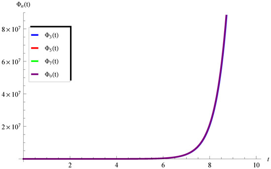
Figure 1.
Plots of the approximations for at , , and .
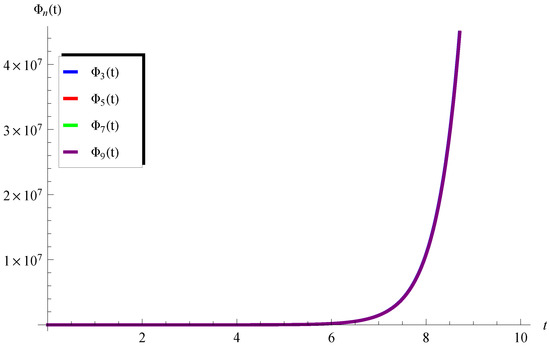
Figure 2.
Plots of the approximations for at , , and .
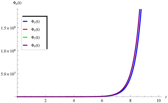
Figure 3.
Plots of the approximations for at , , and .
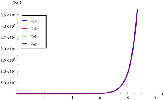
Figure 4.
Plots of the approximations for at , , and .
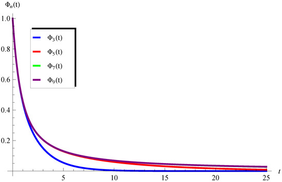
Figure 5.
Plots of the approximations for at , , and .
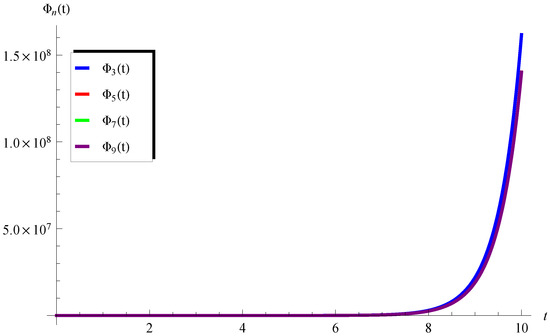
Figure 6.
Plots of the approximations for at , , and .
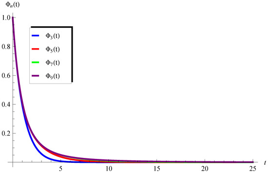
Figure 7.
Plots of the approximations for at , , and .
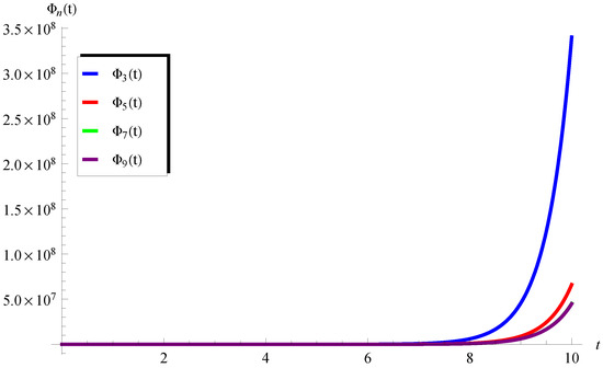
Figure 8.
Plots of the approximations for at , , and .
In the second part of this discussion, we focus on the error analysis. The numerical calculations are performed to estimate the residual errors defined by
For this purpose, the numerical calculations of the residuals , for , are extracted and displayed through Figure 9. The results show an acceptable error and the advantage of the proposed approach is clear, even in a huge domain. This conclusion is confirmed in Figure 10; however, the accuracy enjoys a better performance than the corresponding accuracy in Figure 9. The reason behind that is the increase in the number of terms, where is plotted in Figure 10 at . Of course, one can increase the number of terms as needed to achieve the desired accuracy. In view of the above discussion, one may trust the effectiveness and the efficiency of the LT to treat the PDDE.
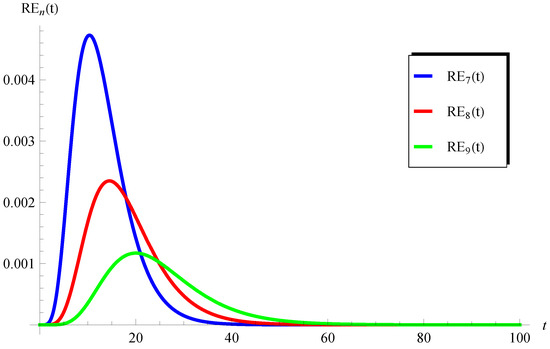
Figure 9.
Variation in the residual for at , , and .
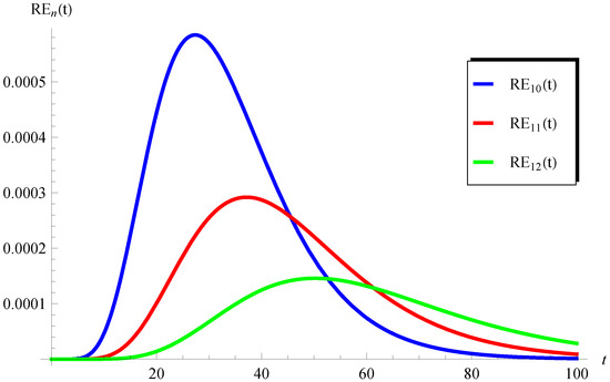
Figure 10.
Variation in the residual for at , , and .
7. Conclusions
In this paper, the PDDE was solved by means of a hybrid approach. The suggested technique was mainly based on combining the LT and the ADM. The analytic approximations were successfully conducted and theoretically proved for convergence. The results in the literature were recovered as special cases of our analysis. The performed numerical calculations confirmed the theoretical theorem of convergence. Furthermore, the calculated residuals reveal the accuracy of the obtained results and also confirm the effectiveness/efficiency of our approach to solve the PDDE. The capability of the present analysis to solve extended versions of the PDDE may deserve further future works.
Author Contributions
Methodology, H.K.A.-J.; Validation, R.A. and H.K.A.-J.; Formal analysis, R.A. and H.K.A.-J.; Investigation, R.A. and H.K.A.-J.; Resources, R.A.; Writing—review & editing, H.K.A.-J. All authors have read and agreed to the published version of the manuscript.
Funding
This research received no external funding.
Conflicts of Interest
The authors declare no conflict of interest.
References
- Ebaid, A.; Alharbi, W.; Aljoufi, M.D.; El-Zahar, E.R. The Exact Solution of the Falling Body Problem in Three-Dimensions: Comparative Study. Mathematics 2020, 8, 1726. [Google Scholar] [CrossRef]
- Aljohani, A.F.; Ebaid, A.; Algehyne, E.A.; Mahrous, Y.M.; Agarwal, P.; Areshi, M.; Al-Jeaid, H.K. On solving the chlorine transport model via Laplace transform. Sci. Rep. 2022, 12, 12154. [Google Scholar] [CrossRef] [PubMed]
- Ebaid, A.; Alali, E.; Saleh, H. The exact solution of a class of boundary value problems with polynomial coefficients and its applications on nanofluids. J. Assoc. Arab. Univ. Basi Appl. Sci. 2017, 24, 156–159. [Google Scholar] [CrossRef]
- Ebaid, A.; Wazwaz, A.M.; Alali, E.; Masaedeh, B. Hypergeometric series solution to a class of second-order boundary value problems via Laplace transform with applications to nanofuids. Commun. Theor. Phys. 2017, 67, 231. [Google Scholar] [CrossRef]
- Ali, H.S.; Alali, E.; Ebaid, A.; Alharbi, F.M. Analytic Solution of a Class of Singular Second-Order Boundary Value Problems with Applications. Mathematics 2019, 7, 172. [Google Scholar] [CrossRef]
- Khaled, S.M.; Ebaid, A.; Al Mutairi, F. The Exact Endoscopic Effect on the Peristaltic Flow of a Nanofluid. J. Appl. Math. 2014, 2014, 367526. [Google Scholar] [CrossRef]
- Ebaid, A.; Al Sharif, M. Application of Laplace transform for the exact effect of a magnetic field on heat transfer of carbon nanotubes suspended nanofluids. Z. Nat. A 2015, 70, 471–475. [Google Scholar] [CrossRef]
- Saleh, H.; Alali, E.; Ebaid, A. Medical applications for the flow of carbon-nanotubes suspended nanofluids in the presence of convective condition using Laplace transform. J. Assoc. Arab. Univ. Basic. Appl. Sci. 2017, 24, 206–212. [Google Scholar] [CrossRef]
- Khaled, S. The exact effects of radiation and joule heating on magnetohydrodynamic Marangoni convection over a flat surface. Therm. Sci. 2018, 22, 63–72. [Google Scholar] [CrossRef]
- Adomian, G. Solving Frontier Problems of Physics: The Decomposition Method; Kluwer Academic Publishers: Boston, MA, USA, 1994. [Google Scholar]
- Wazwaz, A.-M. Adomian decomposition method for a reliable treatment of the Bratu-type equations. Appl. Math. Comput. 2005, 166, 652–663. [Google Scholar] [CrossRef]
- Dehghan, M.; Salehi, R. Solution of a nonlinear time-delay model in biology via semi-analytical approaches. Comput. Phys. Commun. 2010, 181, 1255–1265. [Google Scholar] [CrossRef]
- Ebaid, A. Approximate analytical solution of a nonlinear boundary value problem and its application in fluid mechanics. Z. Nat. A 2011, 66, 423–426. [Google Scholar] [CrossRef]
- Duan, J.-S.; Rach, R. A new modification of the Adomian decomposition method for solving boundary value problems for higher order nonlinear differential equations. Appl. Math. Comput. 2011, 218, 4090–4118. [Google Scholar] [CrossRef]
- Ebaid, A. A new analytical and numerical treatment for singular two-point boundary value problems via the Adomian decomposition method. J. Comput. Appl. Math. 2011, 235, 1914–1924. [Google Scholar] [CrossRef]
- Aly, E.H.; Ebaid, A.; Rach, R. Advances in the Adomian decomposition method for solving two-point nonlinear boundary value problems with Neumann boundary conditions. Comput. Math. Appl. 2012, 63, 1056–1065. [Google Scholar] [CrossRef]
- Chun, C.; Ebaid, A.; Lee, M.; Aly, E.H. An approach for solving singular two point boundary value problems: Analytical and numerical treatment. Anziam J. 2012, 53, 21–43. [Google Scholar] [CrossRef]
- Ebaid, A.; Aljoufi, M.D.; Wazwaz, A.-M. An advanced study on the solution of nanofluid flow problems via Adomian’s method. Appl. Math. Lett. 2015, 46, 117–122. [Google Scholar] [CrossRef]
- Bhalekar, S.; Patade, J. An analytical solution of fishers equation using decomposition Method. Am. J. Comput. Appl. Math. 2016, 6, 123–127. [Google Scholar]
- Alshaery, A.; Ebaid, A. Accurate analytical periodic solution of the elliptical Kepler equation using the Adomian decomposition method. Acta Astronaut. 2017, 140, 27–33. [Google Scholar] [CrossRef]
- Bakodah, H.O.; Ebaid, A. Exact solution of Ambartsumian delay differential equation and comparison with Daftardar-Gejji and Jafari approximate method. Mathematics 2018, 6, 331. [Google Scholar] [CrossRef]
- Ebaid, A.; Al-Enazi, A.; Albalawi, B.Z.; Aljoufi, M.D. Accurate approximate solution of Ambartsumian delay differential equation via decomposition method. Math. Comput. Appl. 2019, 24, 7. [Google Scholar] [CrossRef]
- Li, W.; Pang, Y. Application of Adomian decomposition method to nonlinear systems. Adv. Differ. Equ. 2020, 2020, 67. [Google Scholar] [CrossRef]
- Alenazy, A.H.S.; Ebaid, A.; Algehyne, E.A.; Al-Jeaid, H.K. Advanced Study on the Delay Differential Equation y′(t) = ay(t) + by(ct). Mathematics 2022, 10, 4302. [Google Scholar] [CrossRef]
- Al-Mazmumy, M.; Alsulami, A.A. Solution of Laguerre’s Differential Equations via Modified Adomian Decomposition Method. J. Appl. Math. Phys. 2023, 11, 85–100. [Google Scholar] [CrossRef]
- Abbaoui, K.; Cherruault, Y. Convergence of Adomian’s method applied to nonlinear equations. Math. Comput. Model. 1994, 20, 69–73. [Google Scholar] [CrossRef]
- Cherruault, Y.; Adomian, G. Decomposition Methods: A new proof of convergence. Math. Comput. Model. 1993, 18, 103–106. [Google Scholar] [CrossRef]
- Hosseini, M.M.; Nasabzadeh, H. On the Convergence of Adomian Decomposition Method. Appl. Math. Comput. 2006, 182, 536–543. [Google Scholar] [CrossRef]
- He, J.-H. Homotopy perturbation technique. Comput. Methods Appl. Mech. Eng. 1999, 178, 257–262. [Google Scholar] [CrossRef]
- He, J.-H. Homotopy perturbation method: A new nonlinear analytical technique. Appl. Math. Comput. 2003, 135, 73–79. [Google Scholar] [CrossRef]
- Ganji, A.; Sadighi, A. Application of He’s homotopy-perturbation method to nonlinear coupled systems of reaction-diffusion equations. Int. J. Nonlinear Sci. Numer. Simul. 2006, 7, 411–418. [Google Scholar] [CrossRef]
- Biazar, J.; Ghazvini, H. Convergence of the homotopy perturbation method for partial differential equations. Nonlinear Anal. Real. World Appl. 2009, 10, 2633–2640. [Google Scholar] [CrossRef]
- Turkyilmazoglu, M. Convergence of the homotopy perturbation method. Int. J. Nonlinear Sci. Numer. Simul. 2011, 12, 9–14. [Google Scholar] [CrossRef]
- Khuri, S.A.; Sayfy, A. A Laplace variational iteration strategy for the solution of differential equations. Appl. Math. Lett. 2012, 25, 2298–2305. [Google Scholar] [CrossRef]
- Ebaid, A. Remarks on the homotopy perturbation method for the peristaltic flow of Jeffrey fluid with nano-particles in an asymmetric channel. Comput. Math. Appl. 2014, 68, 77–85. [Google Scholar] [CrossRef]
- Ayati, Z.; Biazar, J. On the convergence of Homotopy perturbation method. J. Egypt. Math. Soc. 2015, 23, 424–428. [Google Scholar] [CrossRef]
- Bayat, M.; Pakar, I.; Bayat, M. Approximate analytical solution of nonlinear systems using homotopy perturbation method. Proc. Inst. Mech. Eng. Part. E J. Process. Mech. Eng. 2014, 230, 10–17. [Google Scholar] [CrossRef]
- Pasha, S.A.; Nawaz, Y.; Arif, M.S. The modified homotopy perturbation method with an auxiliary term for the nonlinear oscillator with discontinuity. J. Low. Freq. Noise Vib. Act. Control 2019, 38, 1363–1373. [Google Scholar] [CrossRef]
- Nadeem, M.; Li, F. He–Laplace method for nonlinear vibration systems and nonlinear wave equations. J. Low. Freq. Noise. Vib. Act. Control 2019, 38, 1060–1074. [Google Scholar] [CrossRef]
- Ebaid, A.; Aljohani, A.F.; Aly, E.H. Homotopy perturbation method for peristaltic motion of gold-blood nanofluid with heat source. Int. J. Numer. Methods Heat. Fluid. Flow. 2019, 30, 3121–3138. [Google Scholar] [CrossRef]
- Ahmad, S.; Ullah, A.; Akgül, A.; De la Sen, M. A Novel Homotopy Perturbation Method with Applications to Nonlinear Fractional Order KdV and Burger Equation with Exponential-Decay Kernel. J. Funct. Spaces 2021, 2021, 8770488. [Google Scholar] [CrossRef]
- He, J.-H.; El-Dib, Y.O.; Mady, A.A. Homotopy Perturbation Method for the Fractal Toda Oscillator. Fractal Fract. 2021, 5, 93. [Google Scholar] [CrossRef]
- Agbata, B.C.; Shior, M.M.; Olorunnishola, O.A.; Ezugorie, I.G.; Obeng-Denteh, W. Analysis of homotopy perturbation method (HPM) and its application for solving infectious disease models. Int. J. Math. Stat. Stud. 2021, 9, 27–38. [Google Scholar]
- Liao, S.J. The Proposed Homotopy Analysis Technique for the Solution of Nonlinear Problems. Ph.D. Thesis, Shanghai Jiao Tong University, Shanghai, China, 1992. [Google Scholar]
- Liao, S. Beyond Perturbation: Introduction to the Homotopy Analysis Method; CRC Press: Boca Raton, FL, USA, 2003. [Google Scholar]
- Liao, S.J. On the homotopy analysis method for nonlinear problems. Appl. Math. Comput. 2004, 147, 499–513. [Google Scholar] [CrossRef]
- Khan, H.; Liao, S.-J.; Mohapatra, R.; Vajravelu, K. An analytical solution for a nonlinear time-delay model in biology. Commun. Nonlinear Sci. Numer. Simul. 2009, 14, 3141–3148. [Google Scholar] [CrossRef]
- Allan, F.M. Derivation of the Adomian decomposition method using the homotopy analysis method. Appl. Math. Comput. 2007, 190, 6–14. [Google Scholar] [CrossRef]
- Abbasbandy, S. Homotopy analysis method for the Kawahara equation. Nonlinear Anal. Real. World Appl. 2010, 11, 307–312. [Google Scholar] [CrossRef]
- Arora, R.; Sharma, H. Application of HAM to seventh order KdV equations. Int. J. Syst. Assur. Eng. Manag. 2018, 9, 131–138. [Google Scholar] [CrossRef]
- Maana, N.; Barde, A. Analytical technique for neutral delay differential equations with proportional and constant delays. J. Math. Comput. Sci. 2020, 20, 334–348. [Google Scholar] [CrossRef]
- Chauhan, A.; Arora, R. Application of homotopy analysis method (HAM) to the non-linear KdV equations. Commun. Math. 2023, 31, 205–220. [Google Scholar] [CrossRef]
- Khan, N.A.; Ara, A.; Yildirim, A.; Yiki, E. Approximate solution of Helmholtz equation by differential transform method. World Appl. Sci. J. 2010, 10, 1490–1492. [Google Scholar]
- Ebaid, A. Approximate periodic solutions for the non-linear relativistic harmonic oscillator via differential transformation method. Commun. Nonlinear Sci. Numer. Simul. 2010, 15, 1921–1927. [Google Scholar] [CrossRef]
- Ebaid, A.E. A reliable aftertreatment for improving the differential transformation method and its application to nonlinear oscillators with fractional nonlinearities. Commun. Nonlinear Sci. Numer. Simul. 2011, 16, 528–536. [Google Scholar] [CrossRef]
- Liu, Y.; Sun, K. Solving power system differential algebraic equations using differential transformation. IEEE Trans. Power Syst. 2020, 35, 2289–2299. [Google Scholar] [CrossRef]
- Benhammouda, B. The differential transform method as an effective tool to solve implicit Hessenberg index-3 differential-algebraic equations. J. Math. 2023, 13, 3620870. [Google Scholar] [CrossRef]
- Spiegel, M.R. Spiegel, Laplace Transforms; McGraw-Hill. Inc.: New York, NY, USA, 1965. [Google Scholar]
- Ebaid, A.; Al-Jeaid, H.K. On the exact solution of the functional differential equation y′(t) = ay(t) + by(−t). Adv. Differ. Equ. Control Process. 2022, 26, 39–49. [Google Scholar] [CrossRef]
- Kac, V.G.; Cheung, P. Quantum Calculus; Springer: New York, NY, USA, 2002. [Google Scholar]
- Albidah, A.B.; Kanaan, N.E.; Ebaid, A.; Al-Jeaid, J.K. Exact and numerical analysis of the pantograph delay differential equation via the homotopy perturbation method. Mathematics 2023, 11, 944. [Google Scholar] [CrossRef]
- El-Zahar, E.R.; Ebaid, A. Analytical and numerical simulations of a delay Model: The Pantograph delay equation. Axioms 2022, 11, 741. [Google Scholar] [CrossRef]


Disclaimer/Publisher’s Note: The statements, opinions and data contained in all publications are solely those of the individual author(s) and contributor(s) and not of MDPI and/or the editor(s). MDPI and/or the editor(s) disclaim responsibility for any injury to people or property resulting from any ideas, methods, instructions or products referred to in the content. |
© 2023 by the authors. Licensee MDPI, Basel, Switzerland. This article is an open access article distributed under the terms and conditions of the Creative Commons Attribution (CC BY) license (https://creativecommons.org/licenses/by/4.0/).