Novel Parametric Families of with and without Memory Iterative Methods for Multiple Roots of Nonlinear Equations

Abstract

The methods that use memory using accelerating parameters for computing multiple roots are almost non-existent in the literature. Furthermore, the only paper available in this direction showed an increase in the order of convergence of 0.5 from the without memory to the with memory extension. In this paper, we introduce a new fifth-order without memory method, which we subsequently extend to two higher-order with memory methods using a self-accelerating parameter. The proposed with memory methods extension demonstrate a significant improvement in the order of convergence from 5 to 7, making this the first paper to achieve at least a 2-order improvement. In addition to this improvement, our paper is also the first to use Hermite interpolating polynomials to approximate the accelerating parameter in the proposed with memory methods for multiple roots. We also provide rigorous theoretical proofs of convergence theorems to establish the order of the proposed methods. Finally, we demonstrate the potential impact of the proposed methods through numerical experimentation on a diverse range of problems. Overall, we believe that our proposed methods have significant potential for various applications in science and engineering.

1. Introduction

The quest for efficient and accurate methods for finding the roots of nonlinear equations is a continuous endeavour in the field of numerical computation. One of the primary objectives in this pursuit is to develop methods that are both efficient and have a simple structure. Iterative methods are favoured for finding the roots of nonlinear equations because they can be easily implemented using computer software and provide results up to a desired accuracy, despite not always yielding exact roots. As a result, they are practical and versatile tools for solving nonlinear equations of the form:

$$\begin{array}{c}\hfill \Omega \left(s_n\right)=0,\end{array}$$

(1)

where $\Omega :D\subseteq \mathbb{C}\to \mathbb{C}$ is a function defined in an open interval D having multiple roots $\xi$ with multiplicity $m>1$. These equations are often encountered in various fields of science, engineering, and mathematics, and their solutions are important for understanding complex systems and phenomena. The modified Newton–Raphson method is a widely known iterative method for finding multiple roots of (1), and it is given by

$$\begin{array}{c}\hfill s_{n+1}=s_n-m\frac{\Omega \left(s_n\right)}{{\Omega }^{\prime }\left(s_n\right)},n=0,1,2,\dots .\end{array}$$

(2)

Equation (2) has a quadratic order of convergence for $m\ge 1$. While there exist numerous with and without memory iterative methods for computing simple roots [1,2,3,4,5,6], the task of developing efficient methods for finding multiple roots remains challenging. Despite the availability of several without memory iterative methods for multiple roots (see [7,8,9,10] and the references therein), there is a paucity of methods that utilise multiple points with memory and accelerating parameters for computing multiple roots.

The authors in [11] recently extended existing optimal-order without memory methods [12,13] for multiple roots to include memory using an accelerating parameter. The with memory extension of the optimal fourth-order method is given below:

$$\begin{array}{cc}\hfill y_n=& s_n-m\frac{\Omega \left(s_n\right)}{{\Omega }^{\prime }\left(s_n\right)+{\alpha }_n\Omega \left(s_n\right)},\hfill \\ \hfill s_{n+1}=& y_n-m{u}_{n}W\left(u_n\right)\frac{\Omega \left(s_n\right)}{{\Omega }^{\prime }\left(s_n\right)+2{\alpha }_n\Omega \left(s_n\right)},\hfill \end{array}$$

(3)

where $u_n={\left(\frac{\Omega \left(y_n\right)}{\Omega \left(s_n\right)}\right)}^{\frac{1}{m}}$. This method (3) has the error equations given by

$$\begin{array}{cc}\hfill e_{n,y}& =\frac{({\alpha }_n+c_1)}{m}{e}_n^2+O\left(e_n^3\right),\hfill \end{array}$$

(4)

$$\begin{array}{cc}\hfill e_{n+1}& =-({\alpha }_n+c_1)\frac{A}{2m^3}{e}_n^4+O\left(e_n^5\right),\hfill \end{array}$$

(5)

where $c_i$=$\frac{m!}{(m+i)!}\frac{{\Omega }^{(m+i)}\left(\xi \right)}{{\Omega }^{\left(m\right)}\left(\xi \right)},i=1,2,\dots$, $e_n=s_n-\xi$ is the error at the $n^{th}$ iteration, $A={\alpha }_n^2(W^{″}\left(0\right)-4)+2{\alpha }_n{c}_1(W^{″}\left(0\right)-7)+(W^{″}\left(0\right)-9-m)c_1^2+2m{c}_2$. The accelerating parameter ${\alpha }_n$ is calculated as follows:

$$\begin{array}{c}\hfill {\alpha }_n=-c_1=-\frac{1}{m+1}\frac{N_2^{(m+1)}\left(s_n\right)}{{\Omega }^{\left(m\right)}\left(s_n\right)},\end{array}$$

(6)

where $N_2^{(m+1)}\left(s_n\right)$ is calculated using a Newton interpolating polynomial.

However, the R-order of convergence of these methods increases from 2 to 2.4142, 4 to 4.2361, and 4 to 4.5616 only, which is a modest improvement. As far as we know, this is the first and only paper that to discuss the with memory iterative method for finding multiple roots using an accelerating parameter.

Motivated by the approach using the self-accelerating technique, we plan to develop new higher-order with memory iterative methods for finding multiple roots of nonlinear equations using an accelerating parameter.

This paper presents new parametric families of two-point with and without memory iterative methods for finding multiple roots of nonlinear equations. The family of without memory methods employs the weight function technique with a real parameter to achieve the fifth order of convergence, while the extended family of with memory methods utilises an accelerating parameter to achieve a two-order improvement in the convergence order. The with memory methods demonstrate an increase in convergence orders from 5 to 7 and 7.2749. To ensure efficiency, we approximated the accelerating parameter using Hermite interpolating polynomials.

The manuscript is structured as follows. Section 2 outlines the development of methods utilising both weight function techniques and the accelerating parameter, with particular attention paid to analysing the order of convergence of the new methods through theorems and lemmas. In Section 3, we present the results of numerical tests comparing the proposed methods with other known methods. Finally, Section 4 provides concluding remarks on the study.

2. Construction of New Iterative Schemes and Their Convergence Analysis

In this section, we present the new parametric families of two-point with and without memory methods for finding multiple roots having multiplicity $m>1$ in two separate subsections.

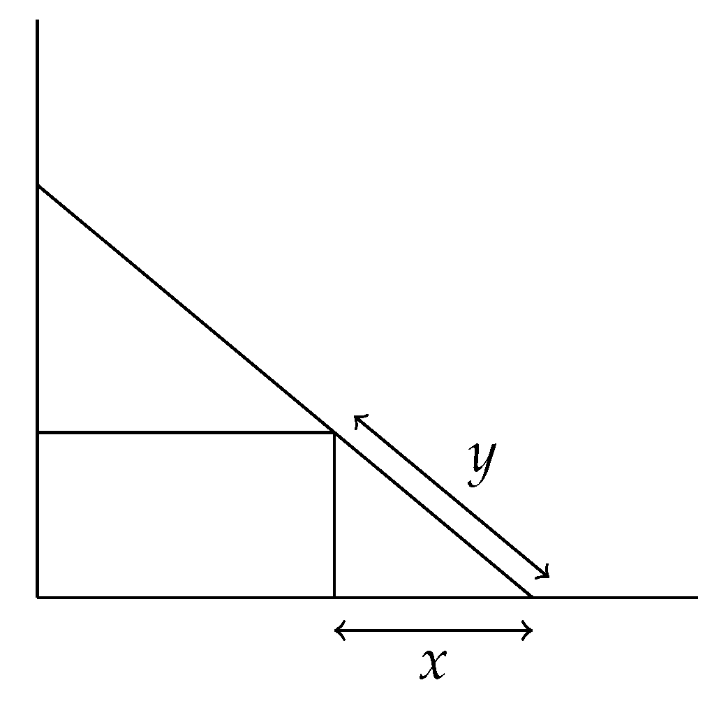
2.1. Parametric Family of Two-Point without Memory Methods and Its Convergence Analysis

Here, we introduce a new fifth-order parametric family of two-point without memory methods for finding multiple roots with multiplicity $m>1$. The newly proposed parametric family of without memory methods is defined as follows, which we denote as PFM:

$$\begin{array}{cc}\hfill y_n& =s_n-m\frac{\Omega \left(s_n\right)}{{\Omega }^{\prime }\left(s_n\right)+\alpha \Omega \left(s_n\right)},\alpha \in \mathbb{R}-\left\{0\right\}\hfill \\ \hfill s_{n+1}& =y_n-mW\left(t_n\right)\frac{\Omega \left(y_n\right)}{{\Omega }^{\prime }\left(y_n\right)+\alpha \Omega \left(y_n\right)},\hfill \end{array}$$

(7)

where $W:\mathbb{C}\to \mathbb{C}$ is an analytic function in the neighbourhood of 0 with $t_n={\left(\frac{{\Omega }^{\prime }\left(y_n\right)}{{\Omega }^{\prime }\left(s_n\right)}\right)}^{\frac{1}{m-1}}$. This new family (7) requires two functions and two first derivative evaluations at each iteration.

Theorem 1.

Let $s=\xi$ be a multiple zero with multiplicity $m>1$ of a function $\Omega :\mathbb{C}\to \mathbb{C}$ in the region enclosing ξ. Then, the new parametric family of methods (PFM) defined by (7) has the fifth order of convergence if the following conditions are fulfilled:

$$W\left(0\right)=1;W^{\prime }\left(0\right)=0;W^{″}\left(0\right)=2;\left|W^{\left(3\right)}\left(0\right)\right|<\infty .$$

(8)

This satisfies the following error equation:

$$\begin{array}{cc}\hfill e_{n+1}=& \frac{{(\alpha +c_1)}^2}{6(m-1)m^4}((1-m)(12m{c}_2+{\alpha }^2(-6+W^{\left(3\right)}\left(0\right)))+2\alpha c_1(m(12-W^{\left(3\right)}\left(0\right))\hfill \\ \hfill & +W^{\left(3\right)}\left(0\right))+c_1^2(6+6m^2-m(-12+W^{\left(3\right)}\left(0\right)+W^{\left(3\right)}\left(0\right))))e_n^5+O\left(e_n^6\right),\hfill \end{array}$$

(9)

where $e_n=s_n-\xi$ is the error at the $n^{th}$ iteration.

Proof of Theorem 1.

Let $s=\xi$ be the multiple roots of $\Omega \left(s\right)=0$ with multiplicity $m>1$ such that $e_n=s_n-\xi$ is the error at the $n^{th}$ iteration. We expand $\Omega \left(s_n\right)$ and ${\Omega }^{\prime }\left(s_n\right)$ in powers of $e_n$ by Taylor’s series expansion as follows:

$$\begin{array}{cc}\hfill \Omega \left(s_n\right)=& \frac{{\Omega }^{\left(m\right)}\left(\xi \right)}{m!}{e}_n^m(1+c_1{e}_n+c_2{e}_n^2+c_3{e}_n^3+c_4{e}_n^4+c_5{e}_n^5+O\left(e_n^6\right)),\hfill \end{array}$$

(10)

$$\begin{array}{cc}\hfill \mathrm{and}{\Omega }^{\prime }\left(s_n\right)=& \frac{{\Omega }^{\left(m\right)}\left(\xi \right)}{m!}{e}_n^{m-1}(m+(m+1)c_1{e}_n+(m+2)c_2{e}_n^2+(m+3)c_3{e}_n^3\hfill \\ \hfill & +(m+4)c_4{e}_n^4+(m+5)c_5{e}_n^5+O\left(e_n^6\right)),\hfill \end{array}$$

(11)

where $c_i=\frac{m!}{(m+i)!}\frac{{\Omega }^{(m+i)}\left(\xi \right)}{{\Omega }^{\left(m\right)}\left(\xi \right)},i=1,2,3,\dots .$ Using the above Equations (10) and (11) in the first step of Equation (7), we obtain

$$\begin{array}{cc}\hfill y_n-\xi =& \frac{\alpha +c_1}{m}{e}_n^2-\frac{1}{m^2}\left({\alpha }^2+2\alpha c_1+(1+m)c_1^2-2m{c}_2\right)e_n^3+\sum _{i=0}^1{S}_i{e}_n^{i+4}+O\left(e_n^6\right),\hfill \end{array}$$

(12)

where $S_i,i=0,1$ are given in terms of $\alpha ,m,c_1,c_2,c_3,c_4$, i.e., $S_0=\frac{1}{m^3}\left({\alpha }^3+(3+2m)\alpha c_1^2+{(1+m)}^2{c}_1^3-4m\alpha c_2+c_1(3{\alpha }^2-m(4+3m)c_2)+3m^2{c}_3\right),S_1=-\frac{1}{m^4}({\alpha }^4+2(2+3m+m^2)\alpha c_1^3+{(1+m)}^3{c}_1^4-6m{\alpha }^2{c}_2+2m^2(2+m)c_2^2-c_1^2(-3(2+m){\alpha }^2+2m(3+5m+2m^2)c_2)+6m^2\alpha c_3+2c_1(2{\alpha }^3-3m(2+m)\alpha c_2+m^2(3+2m)c_3)-4m^3{c}_4)$.

Then, using Equation (12), $\Omega \left(y_n\right)$ and ${\Omega }^{\prime }\left(y_n\right)$ can be obtained as follows:

$$\begin{array}{cc}\hfill \Omega \left(y_n\right)=& \frac{{\Omega }^{\left(m\right)}\left(\xi \right)}{m!}{e}_n^{2m}{\left(\frac{\alpha +c_1}{m}\right)}^m[1-\frac{1}{\alpha +c_1}\left({\alpha }^2+2\alpha c_1+(1+m)c_1^2-2m{c}_2\right)e_n\hfill \\ \hfill & +\sum _{i=0}^3{K}_i{e}_n^{i+2}+O\left(e_n^6\right)],\hfill \end{array}$$

(13)

where $K_i,i=0,1,2,3$ are given in terms of $\alpha ,m,c_1,c_2,c_3,c_4$, i.e.,

$K_0=\frac{1}{2m{(\alpha +c_1)}^2}(2c_1{(\alpha +c_1)}^3+(-1+m){({\alpha }^2+2\alpha c_1+(1+m)c_1^2-2m{c}_2)}^2+2(\alpha +c_1)({\alpha }^3+(3+2m)\alpha c_1^2+{(1+m)}^2{c}_1^3-4m\alpha c_2+c_1(3{\alpha }^2-m(4+3m)c_2)+3m^2{c}_3))$, etc.

In a similar manner, ${\Omega }^{\prime }\left(y_n\right)$ can be written as follows:

$$\begin{array}{cc}\hfill {\Omega }^{\prime }\left(y_n\right)=& \frac{{\Omega }^{\left(m\right)}\left(\xi \right)}{(m-1)!}{\left(\frac{\alpha +c_1}{m}\right)}^{m-1}{e}_n^{2(m-1)}[1-\frac{(m-1)}{m(\alpha +c_1)}({\alpha }^2+2\alpha c_1+(1+m)c_1^2-2m{c}_2)e_n\hfill \\ \hfill & +\sum _{i=0}^3{M}_i{e}_n^{i+2}+O\left(e_n^6\right)],\hfill \end{array}$$

(14)

where $M_i,i=0,1,2,3$ are given in terms of $\alpha ,m,c_1,c_2,c_3,c_4$.

Applying Equations (11) and (14), we obtain

$$\begin{array}{cc}\hfill t_n={\left(\frac{{\Omega }^{\prime }\left(y_n\right)}{{\Omega }^{\prime }\left(s_n\right)}\right)}^{\frac{1}{m-1}}=& \frac{\alpha +c_1}{m}{e}_n+\frac{1}{(m-1)m^2}((\alpha -3m\alpha )c_1-m(1+m)c_1^2\hfill \\ \hfill & +(m-1)(-{\alpha }^2+2m{c}_2))e_n^2+\sum _{i=0}^2{N}_i{e}_n^{i+3}+O\left(e_n^6\right),\hfill \end{array}$$

(15)

where $N_i,i=0,1,2$ are given in terms of $\alpha ,m,c_1,c_2,c_3,c_4$.

Expanding the weight function $W\left(t_n\right)$ in the neighbourhood of origin by Taylor’s series expansion up to second-order terms gives

$$\begin{array}{c}\hfill W\left(t_n\right)\approx W\left(0\right)+t_n{W}^{\prime }\left(0\right)+\frac{t_n^2}{2!}{W}^{″}\left(0\right).\end{array}$$

(16)

Now, substituting the expressions (12)–(16) in the last step of Equation (7), the error equation is obtained as follows:

$$\begin{array}{cc}\hfill e_{n+1}=& \frac{1}{m}(1-W\left(0\right))(\alpha +c_1)e_n^2+\frac{1}{m^2}(2m(1-W\left(0\right))c_2+{\alpha }^2(-1+W\left(0\right)\hfill \\ \hfill & -W^{\prime }\left(0\right))+2\alpha c_1(-1+W\left(0\right)-W^{\prime }\left(0\right))+c_1^2(-1+m(-1+W\left(0\right))\hfill \\ \hfill & +W\left(0\right)-W^{\prime }\left(0\right)))e_n^3+\dots +O\left(e_n^6\right).\hfill \end{array}$$

(17)

Now, putting the conditions $W\left(0\right)=1$, $W^{\prime }\left(0\right)=0$, and $W^{″}\left(0\right)=2$ in (17), the error equation becomes

$$\begin{array}{cc}\hfill e_{n+1}=& \frac{{(\alpha +c_1)}^2}{6(m-1)m^4}((1-m)(12m{c}_2+{\alpha }^2(-6+W^{\left(3\right)}\left(0\right)))+2\alpha c_1(m(12-W^{\left(3\right)}\left(0\right))\hfill \\ \hfill & +W^{\left(3\right)}\left(0\right))+c_1^2(6+6m^2-m(-12+W^{\left(3\right)}\left(0\right)+W^{\left(3\right)}\left(0\right))))e_n^5+O\left(e_n^6\right).\hfill \end{array}$$

From the above error equation, we can conclude that the newly proposed family of iterative methods (PFM) is of fifth order. This completes the proof. □

Some Particular Cases of the Weight Function, $W\left(t_n\right)$:

Based on the conditions on $W\left(t_n\right)$ as shown in Theorem 1, we can generate numerous methods of the family (7). However, we restricted this to the following simple forms:

Case 1. Let $W\left(t_n\right)$ be a polynomial function of degree two of the form:

$$\begin{array}{c}\hfill W\left(t_n\right)=a_0+a_1{t}_n+a_2{t}_n^2.\end{array}$$

Then, using the conditions (8) of Theorem 1, we obtain $a_0=a_2=1$ and $a_1=0$. Thus, $W\left(t_n\right)$ becomes

$$\begin{array}{c}\hfill W\left(t_n\right)=1+t_n^2.\end{array}$$

(18)

Case 2. Consider $W\left(t_n\right)$ as a rational function of the form:

$$\begin{array}{c}\hfill W\left(t_n\right)=\frac{1+a_0{t}_n}{1+a_1{t}_n+a_2{t}_n^2}.\end{array}$$

Then, using the conditions (8) of Theorem 1, we obtain $a_0=a_1=\lambda$ and $a_2=-1$. Thus, $W\left(t_n\right)$ becomes

$$\begin{array}{c}\hfill W\left(t_n\right)=\frac{1+\lambda t_n}{1+\lambda t_n-t_n^2},\lambda \in \mathbb{R}.\end{array}$$

(19)

Case 3. Let $W\left(t_n\right)$ be another rational function of the form:

$$\begin{array}{c}\hfill W\left(t_n\right)=\frac{1+a_0{t}_n^2}{1+a_1{t}_n^2}.\end{array}$$

Then, using the conditions (8) of Theorem 1, we obtain $a_0=2$ and $a_1=1$. Thus, $W\left(t_n\right)$ becomes

$$\begin{array}{c}\hfill W\left(t_n\right)=\frac{1+2t_n^2}{1+t_n^2}.\end{array}$$

(20)

Case 4. Let $W\left(t_n\right)$ be a function of the form:

$$\begin{array}{c}\hfill W\left(t_n\right)=(1-t_n)e^{a_0{t}_n}+a_1{t}_n^2.\end{array}$$

Then, using the conditions (8) of Theorem 1, we obtain $a_0=1$ and $a_1=\frac{3}{2}$. Thus, $W\left(t_n\right)$ becomes

$$\begin{array}{c}\hfill W\left(t_n\right)=(1-t_n)e^{t_n}+\frac{3}{2}{t}_n^2.\end{array}$$

(21)

2.2. Parametric Families of Two-Point with Memory Methods and Their Convergence Analysis

Here, we propose new parametric families of two-point with memory methods, which are an extension of the new fifth-order parametric family of without memory methods (PFM) (7).

By analysing the error Equation (9) of Theorem 1, we found that the convergence order of PFM (7) can be increased from 5 to 7 if we set $\alpha =-c_1$, where $c_1=\frac{m!}{(m+1)!}\frac{{\Omega }^{(m+1)}\left(\xi \right)}{{\Omega }^{\left(m\right)}\left(\xi \right)}$, $m>1$. However, since the exact values of ${\Omega }^{(m+1)}\left(\xi \right)$ and ${\Omega }^{\left(m\right)}\left(\xi \right)$ are not available, we used some approximations and replaced $\alpha$ by ${\alpha }_n$, where ${\alpha }_n$ is an accelerating parameter computed using available information from the current and previous iterations to satisfy the following condition:

$$\begin{array}{c}\hfill \underset{n\to \infty }{lim}{\alpha }_n=-\frac{m!}{(m+1)!}\frac{{\Omega }^{(m+1)}\left(\xi \right)}{{\Omega }^{\left(m\right)}\left(\xi \right)}.\end{array}$$

(22)

To be precise, we employed Hermite interpolating polynomial for the computation of ${\alpha }_n$ as follows:

FORM 1. We computed ${\alpha }_n$ as follows:

$$\begin{array}{c}\hfill {\alpha }_n=-\frac{{\mathbb{H}}_3^{(m+1)}\left(s_n\right)}{(m+1){\Omega }^{\left(m\right)}\left(s_n\right)},\end{array}$$

(23)

where

$$\begin{array}{cc}\hfill {\mathbb{H}}_3\left(s\right)=& \Omega \left(s_n\right)+\Omega [s_n,s_n](s-s_n)+\Omega [s_n,s_n,s_n]{(s-s_n)}^2+\cdots +\Omega [\underset{m+1}{\underbrace{s_n,s_n,s_n,\dots ,s_n}},y_{n-1}]\times \hfill \\ \hfill & {(s-s_n)}^{m+1}+\Omega [\underset{m+1}{\underbrace{s_n,s_n,s_n,\dots ,s_n}},y_{n-1},y_{n-1}]{(s-s_n)}^{m+1}(s-y_{n-1})\hfill \\ \hfill & +\Omega [\underset{m+1}{\underbrace{s_n,s_n,s_n,\dots ,s_n}},y_{n-1},y_{n-1},s_{n-1}]{(s-s_n)}^{m+1}{(s-y_{n-1})}^2\hfill \end{array}$$

and

$$\begin{array}{cc}\hfill {\mathbb{H}}_3^{(m+1)}\left(s_n\right)=& \Omega [\underset{m+1}{\underbrace{s_n,s_n,s_n,\dots ,s_n}},y_{n-1}](m+1)!+\Omega [\underset{m+1}{\underbrace{s_n,s_n,s_n,\dots ,s_n}},y_{n-1},y_{n-1}](m+1)!\times \hfill \\ \hfill & (s_n-y_{n-1})+\Omega [\underset{m+1}{\underbrace{s_n,s_n,s_n,\dots ,s_n}},y_{n-1},y_{n-1},s_{n-1}](m+1)!{(s_n-y_{n-1})}^2.\hfill \end{array}$$

Remark 1.

The Hermite interpolating polynomial ${\mathbb{H}}_k\left(s\right),k=3,4$ satisfies the condition ${\mathbb{H}}_k^{{}^{\prime }}\left(s_n\right)={\Omega }^{\prime }\left(s_n\right),k=3,4$.

Now, substituting ${\alpha }_n$ from (23) in Equation (7), we obtain the following parametric family of with memory methods, which we denote as PFWM1:

$$\begin{array}{cc}\hfill y_n& =s_n-m\frac{\Omega \left(s_n\right)}{{\Omega }^{\prime }\left(s_n\right)+{\alpha }_n\Omega \left(s_n\right)},{\alpha }_n=-\frac{{\mathbb{H}}_3^{(m+1)}\left(s_n\right)}{(m+1){\Omega }^{\left(m\right)}\left(s_n\right)},\hfill \\ \hfill s_{n+1}& =y_n-mW\left(t_n\right)\frac{\Omega \left(y_n\right)}{{\Omega }^{\prime }\left(y_n\right)+{\alpha }_n\Omega \left(y_n\right)}.\hfill \end{array}$$

(24)

FORM 2. We computed ${\alpha }_n$ as follows:

$$\begin{array}{c}\hfill {\alpha }_n=-\frac{{\mathbb{H}}_4^{(m+1)}\left(s_n\right)}{(m+1){\Omega }^{\left(m\right)}\left(s_n\right)},\end{array}$$

(25)

where

$$\begin{array}{cc}\hfill {\mathbb{H}}_4\left(s\right)=& \Omega \left(s_n\right)+\Omega [s_n,s_n](s-s_n)+\Omega [s_n,s_n,s_n]{(s-s_n)}^2+\cdots +\hfill \\ \hfill & \Omega [\underset{m+1}{\underbrace{s_n,s_n,s_n,\dots ,s_n}},y_{n-1}]{(s-s_n)}^{m+1}+\Omega [\underset{m+1}{\underbrace{s_n,s_n,s_n,\dots ,s_n}},y_{n-1},y_{n-1}]{(s-s_n)}^{m+1}\times \hfill \\ \hfill & (s-y_{n-1})+\Omega [\underset{m+1}{\underbrace{s_n,s_n,s_n,\dots ,s_n}},y_{n-1},y_{n-1},s_{n-1}]{(s-s_n)}^{m+1}{(s-y_{n-1})}^2\hfill \\ \hfill & +\Omega [\underset{m+1}{\underbrace{s_n,s_n,s_n,\dots ,s_n}},y_{n-1},y_{n-1},s_{n-1},s_{n-1}]{(s-s_n)}^{m+1}{(s-y_{n-1})}^2(s-s_{n-1})\hfill \end{array}$$

and

$$\begin{array}{cc}\hfill {\mathbb{H}}_4^{(m+1)}\left(s_n\right)=& \Omega [\underset{m+1}{\underbrace{s_n,s_n,s_n,\dots ,s_n}},y_{n-1}](m+1)!+\Omega [\underset{m+1}{\underbrace{s_n,s_n,s_n,\dots ,s_n}},y_{n-1},y_{n-1}](m+1)!\times \hfill \\ \hfill & (s_n-y_{n-1})+\Omega [\underset{m+1}{\underbrace{s_n,s_n,s_n,\dots ,s_n}},y_{n-1},y_{n-1},s_{n-1}](m+1)!{(s_n-y_{n-1})}^2\hfill \\ \hfill & +\Omega [\underset{m+1}{\underbrace{s_n,s_n,s_n,\dots ,s_n}},y_{n-1},y_{n-1},s_{n-1},s_{n-1}](m+1)!{(s_n-y_{n-1})}^2(s_n-s_{n-1}).\hfill \end{array}$$

Now, substituting ${\alpha }_n$ from (25) in Equation (7), we obtain the following parametric family of with memory methods, which we denote as PFWM2:

$$\begin{array}{cc}\hfill y_n& =s_n-m\frac{\Omega \left(s_n\right)}{{\Omega }^{\prime }\left(s_n\right)+{\alpha }_n\Omega \left(s_n\right)},{\alpha }_n=-\frac{{\mathbb{H}}_4^{(m+1)}\left(s_n\right)}{(m+1){\Omega }^{\left(m\right)}\left(s_n\right)},\hfill \\ \hfill s_{n+1}& =y_n-mW\left(t_n\right)\frac{\Omega \left(y_n\right)}{{\Omega }^{\prime }\left(y_n\right)+{\alpha }_n\Omega \left(y_n\right)}.\hfill \end{array}$$

(26)

Thus, PFWM1 and PFWM2 preserve the efficiency properties of the corresponding without memory methods (PFM) and result in the increase of the convergence order of the with memory methods from 5 to at least 7, resulting in at least a 2-order improvement.

Lemma 1.

If ${\alpha }_n=-\frac{{\mathbb{H}}_3^{(m+1)}\left(s_n\right)}{(m+1){\Omega }^{\left(m\right)}\left(s_n\right)},n=1,2,3,\dots$, then the given estimation:

$${\alpha }_n+c_1\sim c_4{e}_{n-1,y}^2{e}_{n-1}$$

(27)

holds, where $e_n=s_n-\xi$, $e_{n,y}=y_n-\xi$, and $c_4$ is an asymptotic constant.

Proof of Lemma 1.

The error of Hermite interpolation can be expressed as follows:

$$\Omega \left(s\right)-{\mathbb{H}}_3\left(s\right)=\frac{{\Omega }^{(m+4)}\left(\delta \right)}{(m+4)!}{(s-s_n)}^{(m+1)}{(s-y_{n-1})}^2(s-s_{n-1}).$$

(28)

Now, after differentiating (28) $(m+1)$ times at the point $s=s_n$ and rearranging, we obtain the expression:

$${\mathbb{H}}_3^{(m+1)}\left(s_n\right)={\Omega }^{(m+1)}\left(s_n\right)-\frac{{\Omega }^{(m+4)}\left(\delta \right)}{(m+4)!}(m+1)!{(s_n-y_{n-1})}^2(s_n-s_{n-1}).$$

(29)

Now, for the multiple roots $\xi$, we have the following Taylor series of function $\Omega$ at the point $s_n$:

$$\Omega \left(s_n\right)=\frac{{\Omega }^{\left(m\right)}\left(\xi \right)}{m!}\left(e_n^m+c_1{e}_n^{m+1}+c_2{e}_n^{m+2}+c_3{e}_n^{m+3}+O\left(e_n^{m+4}\right)\right).$$

(30)

Then, after differentiating $(m+1)$ times, we have

$${\Omega }^{(m+1)}\left(s_n\right)=\frac{{\Omega }^{\left(m\right)}\left(\xi \right)}{m!}\left((m+1)!c_1+(m+2)!c_2{e}_n+O\left(e_n^2\right)\right).$$

(31)

Similarly,

$${\Omega }^{(m+4)}\left(\delta \right)=\frac{{\Omega }^{\left(m\right)}\left(\xi \right)}{m!}\left((m+4)!c_4+(m+5)!c_5{e}_{\delta }+O\left(e_{\delta }^2\right)\right),$$

(32)

where $e_{\delta }=\delta -\xi$. Thus, using Equations (31) and (32) in (29) and excluding the terms of $e_n$ and $e_{\delta }$, we can obtain

$$\begin{array}{cc}\hfill {\mathbb{H}}_3^{(m+1)}\left(s_n\right)\sim & \frac{{\Omega }^{\left(m\right)}\left(\xi \right)}{m!}(m+1)!c_1-\frac{{\Omega }^{\left(m\right)}\left(\xi \right)}{m!}{c}_4(m+1)!{(s_n-y_{n-1})}^2(s_n-s_{n-1}).\hfill \end{array}$$

(33)

After solving this, we have

$$\begin{array}{c}\hfill {\mathbb{H}}_3^{(m+1)}\left(s_n\right)\sim {\Omega }^{\left(m\right)}\left(\xi \right)\left(m+1\right)\left(c_1-c_4{(s_n-y_{n-1})}^2(s_n-s_{n-1})\right),\end{array}$$

(34)

which implies

$$\begin{array}{c}\hfill -\frac{{\mathbb{H}}_3^{(m+1)}\left(s_n\right)}{(m+1){\Omega }^{\left(m\right)}\left(s_n\right)}\sim -\left(c_1-c_4{(s_n-y_{n-1})}^2(s_n-s_{n-1})\right)\end{array}$$

(35)

or

$$\begin{array}{c}\hfill {\alpha }_n\sim -c_1+c_4{(s_n-y_{n-1})}^2(s_n-s_{n-1}).\end{array}$$

(36)

Finally, we have

$${\alpha }_n+c_1\sim c_4{e}_{n-1,y}^2{e}_{n-1}.$$

(37)

This completes the proof for Lemma 1. □

Theorem 2.

Suppose $\Omega :\mathbb{C}\to \mathbb{C}$ is a function in the neighbourhood of the multiple roots ξ of $\Omega \left(s\right)=0$ of multiplicity $m>1$. If $s_0$ is sufficiently close to ξ, then the R-order of convergence of the iterative method (24) with the parameter ${\alpha }_n$ calculated by (23) is at least seven.

Proof of Theorem 2.

Let the iterative method (IM) generates the sequence of $\left\{s_n\right\}$, which converges to the root $\xi$ of $\Omega \left(s\right)$; by means of R-order $O_R(IM,\xi )\ge r$, we express

$$\begin{array}{cc}\hfill e_{n+1}\sim & D_{n,r}{e}_n^r\hfill \end{array}$$

(38)

and

$$\begin{array}{cc}\hfill e_n\sim & D_{n-1,r}{e}_{n-1}^r.\hfill \end{array}$$

(39)

Next, $D_{n,r}$ will tend to the asymptotic error constant $D_r$ of $IM$ by taking $n\to \infty$. Then,

$$e_{n+1}\sim D_{n,r}{\left(D_{n-1,r}{e}_{n-1}^r\right)}^r=D_{n,r}{D}_{n-1,r}^r{e}_{n-1}^{r^2}.$$

(40)

The resulting error expression of the with memory scheme (24) can be obtained using (12) and (9) and the varying parameter ${\alpha }_n$ as follows:

$$\begin{array}{c}\hfill e_{n,y}=y_n-\xi \sim \frac{{\alpha }_n+c_1}{m}{e}_n^2\end{array}$$

(41)

and

$$\begin{array}{cc}\hfill e_{n+1}=s_{n+1}-\xi \sim & \frac{1}{6(m-1)m^4}{({\alpha }_n+c_1)}^2((1-m)(12m{c}_2+{\alpha }_n^2(-6+W^{\left(3\right)}\left(0\right)))\hfill \\ \hfill & +2{\alpha }_n{c}_1(m(12-W^{\left(3\right)}\left(0\right))+W^{\left(3\right)}\left(0\right))+c_1^2(6+6m^2\hfill \\ \hfill & -m(-12+W^{\left(3\right)}\left(0\right)+W^{\left(3\right)}\left(0\right))\left)\right)e_n^5.\hfill \end{array}$$

(42)

Here, the higher-order terms in Equations (41) and (42) are excluded.

Now, let p be the R-order of convergence of the iterative sequence $\left\{y_n\right\}$. Then,

$$e_{n,y}\sim D_{n,p}{e}_n^p\sim D_{n,p}{\left(D_{n-1,r}{e}_{n-1}^r\right)}^p\sim D_{n,p}{D}_{n-1,r}^p{e}_{n-1}^{rp}$$

(43)

and

$$e_{n-1,y}\sim D_{n-1,p}{e}_{n-1}^p.$$

(44)

Now, by Equations (37), (41) and (44), we obtain

$$\begin{array}{cc}\hfill e_{n,y}\sim \frac{{\alpha }_n+c_1}{m}{e}_n^2& \sim \left(\frac{c_4{e}_{n-1,y}^2{e}_{n-1}}{m}\right){\left(D_{n-1,r}{e}_{n-1}^r\right)}^2\hfill \\ \hfill & \sim \left(\frac{c_4{\left(D_{n-1,p}{e}_{n-1}^p\right)}^2{e}_{n-1}}{m}\right){\left(D_{n-1,r}{e}_{n-1}^r\right)}^2\hfill \\ \hfill & \sim \frac{c_4{D}_{n-1,p}^2{D}_{n-1,r}^2}{m}{e}_{n-1}^{2p+2r+1}.\hfill \end{array}$$

(45)

Again, by (37), (42) and (44), we have

$$\begin{array}{cc}\hfill e_{n+1}& \sim \frac{1}{6(m-1)m^4}{({\alpha }_n+c_1)}^2{G}_n{e}_n^5\hfill \\ \hfill & \sim \frac{1}{6(m-1)m^4}{\left(c_4{e}_{n-1,y}^2{e}_{n-1}\right)}^2{G}_n{\left(D_{n-1,r}{e}_{n-1}^r\right)}^5\hfill \\ \hfill & \sim \frac{1}{6(m-1)m^4}{\left(c_4{\left(D_{n-1,p}{e}_{n-1}^p\right)}^2{e}_{n-1}\right)}^2{G}_n{\left(D_{n-1,r}{e}_{n-1}^r\right)}^5\hfill \\ \hfill & \sim \frac{1}{6(m-1)m^4}\left(c_4^2{D}_{n-1,p}^4{G}_n{D}_{n-1,r}^5\right)e_{n-1}^{4p+5r+2},\hfill \end{array}$$

(46)

where $G_n$ originates from (42).

Since $r>p$, by equating the exponents of $e_{n-1}$ present in the set of relations (43)–(45) and (40)–(46), we attain the resulting system of equations:

$$\begin{array}{cc}\hfill rp& =2r+2p+1,\hfill \\ \hfill r^2& =5r+4p+2.\hfill \end{array}$$

(47)

The positive solutions of the system of Equation (47) are $r=7$ and $p=3$. As a result, the R-order of convergence of the with memory iterative method (24) is at least $r=7$. □

Lemma 2.

If ${\alpha }_n=-\frac{{\mathbb{H}}_4^{(m+1)}\left(s_n\right)}{(m+1){\Omega }^{\left(m\right)}\left(s_n\right)},n=1,2,3,\dots$, then the given estimation:

$${\alpha }_n+c_1\sim c_5{e}_{n-1,y}^2{e}_{n-1}^2$$

(48)

holds, where $e_n=s_n-\xi$, $e_{n,y}=y_n-\xi$, and $c_5$ is an asymptotic constant.

Proof of Lemma 2.

The error of Hermite interpolation can be expressed as follows:

$$\Omega \left(s\right)-{\mathbb{H}}_4\left(s\right)=\frac{{\Omega }^{(m+5)}\left(\delta \right)}{(m+5)!}{(s-s_n)}^{(m+1)}{(s-y_{n-1})}^2{(s-s_{n-1})}^2.$$

(49)

Then, after differentiating (49) $(m+1)$ times at the point $s=s_n$ and rearranging, we obtain the expression below:

$${\mathbb{H}}_4^{(m+1)}\left(s_n\right)={\Omega }^{(m+1)}\left(s_n\right)-\frac{{\Omega }^{(m+5)}\left(\delta \right)}{(m+5)!}(m+1)!{(s_n-y_{n-1})}^2{(s_n-s_{n-1})}^2.$$

(50)

Now, for the multiple roots $\xi$, we have the following Taylor series of function $\Omega$ at the point $s_n$:

$$\Omega \left(s_n\right)=\frac{{\Omega }^{\left(m\right)}\left(\xi \right)}{m!}\left(e_n^m+c_1{e}_n^{m+1}+c_2{e}_n^{m+2}+c_3{e}_n^{m+3}+O\left(e_n^{m+4}\right)\right).$$

(51)

Then, after differentiating $(m+1)$ times, we have

$${\Omega }^{(m+1)}\left(s_n\right)=\frac{{\Omega }^{\left(m\right)}\left(\xi \right)}{m!}((m+1)!c_1+(m+2)!c_2{e}_n+O\left(e_n^2\right)).$$

(52)

Similarly,

$${\Omega }^{(m+5)}\left(\delta \right)=\frac{{\Omega }^{\left(m\right)}\left(\xi \right)}{m!}((m+5)!c_5+(m+6)!c_6{e}_{\delta }+O\left(e_{\delta }^2\right)),$$

(53)

where $e_{\delta }=\delta -\xi$. Thus, using Equations (52) and (53) in (50) and excluding the terms of $e_n$ and $e_{\delta }$, we can obtain

$$\begin{array}{cc}\hfill {\mathbb{H}}_4^{(m+1)}\left(s_n\right)\sim & \frac{{\Omega }^{\left(m\right)}\left(\xi \right)}{m!}(m+1)!c_1-\frac{{\Omega }^{\left(m\right)}\left(\xi \right)}{m!}{c}_5(m+1)!{(s_n-y_{n-1})}^2{(s_n-s_{n-1})}^2.\hfill \end{array}$$

(54)

After solving this, we have

$$\begin{array}{c}\hfill {\mathbb{H}}_4^{(m+1)}\left(s_n\right)\sim {\Omega }^{\left(m\right)}\left(\xi \right)\left(m+1\right)\left(c_1-c_5{(s_n-y_{n-1})}^2{(s_n-s_{n-1})}^2\right),\end{array}$$

(55)

which implies

$$\begin{array}{c}\hfill -\frac{{\mathbb{H}}_4^{(m+1)}\left(s_n\right)}{(m+1){\Omega }^{\left(m\right)}\left(s_n\right)}\sim -\left(c_1-c_5{(s_n-y_{n-1})}^2{(s_n-s_{n-1})}^2\right)\end{array}$$

(56)

or

$$\begin{array}{c}\hfill {\alpha }_n\sim -c_1+c_5{(s_n-y_{n-1})}^2{(s_n-s_{n-1})}^2.\end{array}$$

(57)

Finally, we have

$${\alpha }_n+c_1\sim c_5{e}_{n-1,y}^2{e}_{n-1}^2.$$

(58)

This completes the proof for Lemma 2. □

Theorem 3.

Suppose $\Omega :\mathbb{C}\to \mathbb{C}$ is a function in the neighbourhood of the multiple roots ξ of $\Omega \left(s\right)=0$ of multiplicity $m>1$. If $s_0$ is sufficiently close to ξ, then the R-order of convergence of the iterative method (26) with the parameter ${\alpha }_n$ calculated by (25) is at least $(7+\sqrt{57})/2\approx 7.2749$.

Proof of Theorem 3.

Let the iterative method (IM) generates the sequence of $\left\{s_n\right\}$, which converges to the root $\xi$ of $\Omega \left(s\right)$; by means of R-order $O_R(IM,\xi )\ge r$, we express

$$\begin{array}{cc}\hfill e_{n+1}\sim & D_{n,r}{e}_n^r\hfill \end{array}$$

(59)

and

$$\begin{array}{cc}\hfill e_n\sim & D_{n-1,r}{e}_{n-1}^r.\hfill \end{array}$$

(60)

Next, $D_{n,r}$ will tend to the asymptotic error constant $D_r$ of $IM$ by taking $n\to \infty$. Then,

$$e_{n+1}\sim D_{n,r}{\left(D_{n-1,r}{e}_{n-1}^r\right)}^r=D_{n,r}{D}_{n-1,r}^r{e}_{n-1}^{r^2}.$$

(61)

The resulting error expression of the with memory scheme (26) can be obtained using (12) and (9) and the varying parameter ${\alpha }_n$ as follows:

$$\begin{array}{c}\hfill e_{n,y}=y_n-\xi \sim \frac{{\alpha }_n+c_1}{m}{e}_n^2\end{array}$$

(62)

and

$$\begin{array}{cc}\hfill e_{n+1}=s_{n+1}-\xi \sim & \frac{1}{6(m-1)m^4}{({\alpha }_n+c_1)}^2((1-m)(12m{c}_2\hfill \\ \hfill & +{\alpha }_n^2(-6+W^{\left(3\right)}\left(0\right)))+2{\alpha }_n{c}_1(m(12-W^{\left(3\right)}\left(0\right))+W^{\left(3\right)}\left(0\right))\hfill \\ \hfill & +c_1^2(6+6m^2-m(-12+W^{\left(3\right)}\left(0\right)+W^{\left(3\right)}(0))))e_n^5.\hfill \end{array}$$

(63)

Here, the higher-order terms in Equations (62) and (63) are excluded.

Now, let p be the R-order convergence of the iterative sequences $\left\{y_n\right\}$. Then,

$$e_{n,y}\sim D_{n,p}{e}_n^p\sim D_{n,p}{\left(D_{n-1,r}{e}_{n-1}^r\right)}^p\sim D_{n,p}{D}_{n-1,r}^p{e}_{n-1}^{rp}$$

(64)

and

$$e_{n-1,y}\sim D_{n-1,p}{e}_{n-1}^p.$$

(65)

Then, by Equations (58), (62) and (65), we obtain

$$\begin{array}{cc}\hfill e_{n,y}\sim \frac{{\alpha }_n+c_1}{m}{e}_n^2& \sim \left(\frac{c_5{e}_{n-1,y}^2{e}_{n-1}^2}{m}\right){\left(D_{n-1,r}{e}_{n-1}^r\right)}^2\hfill \\ \hfill & \sim \left(\frac{c_5{\left(D_{n-1,p}{e}_{n-1}^p\right)}^2{e}_{n-1}^2}{m}\right){\left(D_{n-1,r}{e}_{n-1}^r\right)}^2\hfill \\ \hfill & \sim \frac{c_5{D}_{n-1,p}^2{D}_{n-1,r}^2}{m}{e}_{n-1}^{2p+2r+2}.\hfill \end{array}$$

(66)

Again, by (58), (63) and (65), we have

$$\begin{array}{cc}\hfill e_{n+1}& \sim \frac{1}{6(m-1)m^4}{({\alpha }_n+c_1)}^2{G}_n{e}_n^5\hfill \\ \hfill & \sim \frac{1}{6(m-1)m^4}{\left(c_5{e}_{n-1,y}^2{e}_{n-1}^2\right)}^2{G}_n{\left(D_{n-1,r}{e}_{n-1}^r\right)}^5\hfill \\ \hfill & \sim \frac{1}{6(m-1)m^4}{\left(c_5{\left(D_{n-1,p}{e}_{n-1}^p\right)}^2{e}_{n-1}^2\right)}^2{G}_n{\left(D_{n-1,r}{e}_{n-1}^r\right)}^5\hfill \\ \hfill & \sim \frac{1}{6(m-1)m^4}\left(c_5^2{D}_{n-1,p}^4{G}_n{D}_{n-1,r}^5\right)e_{n-1}^{4p+5r+4},\hfill \end{array}$$

(67)

where $G_n$ originates from (63).

Since $r>p$, by equating the exponents of $e_{n-1}$ present in the set of relations (64)–(66) and (61)–(67), we attain the resulting system of equations:

$$\begin{array}{cc}\hfill rp& =2r+2p+2,\hfill \\ \hfill r^2& =5r+4p+4.\hfill \end{array}$$

(68)

The positive solutions of the system of Equation (68) are $r=(7+\sqrt{57})/2$ and $p=(5+\sqrt{57})/4$. As a result, the R-order of convergence of the with memory iterative method (26) is at least $r=(7+\sqrt{57})/2\approx 7.2749$. □

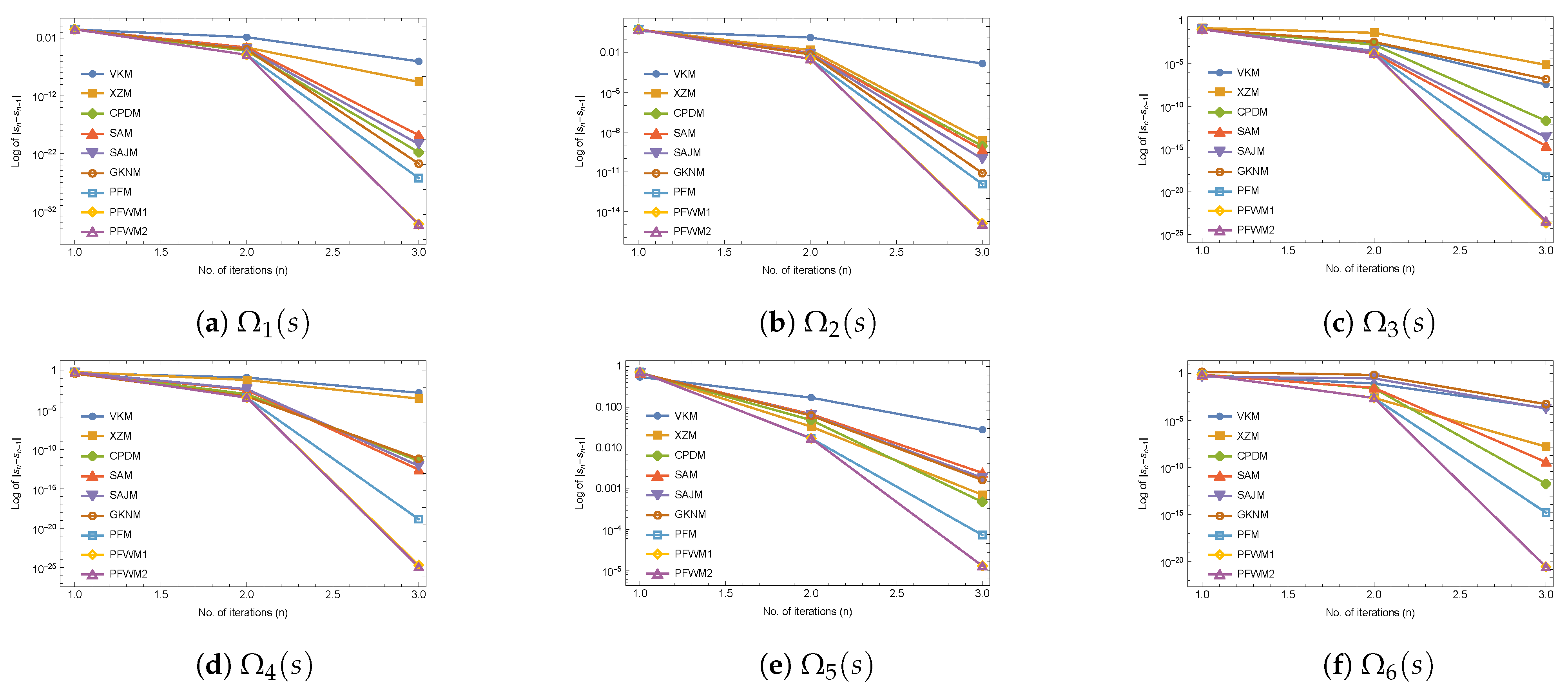
3. Numerical Results

In this section, we assess the performance and computational efficiency of the newly developed families of methods PFM, PFWM1 and PFWM2, which were discussed in Section 2. As for the weight function $W\left(t_n\right)$, we use the particular case given in Equation (18) throughout the whole computation. Additionally, we compare these methods with other similar approaches described in existing literature. The objective of this analysis is to provide a comprehensive evaluation of the proposed families of methods and to validate their theoretical results. By conducting this comparison, we aim to gain a better understanding of the effectiveness and practicality of these new methods and their potential utility for various applications.

Now, let us consider some existing methods for finding multiple roots available in literature for the comparison.

A subcase of the third-order method given by Vinay Kanwar et al. [7], which was developed in March, 2023. The method is denoted as VKM, and the expression is given below:

$$\begin{array}{c}\hfill s_{n+1}=s_n-\left(\frac{2}{2-L_f}\right)\frac{m\Omega \left(s_n\right)}{{\Omega }^{\prime }\left(s_n\right)-m\lambda \Omega \left(s_n\right)},\end{array}$$

(69)

where $\lambda =1$, $L_f=\frac{m\Omega \left(s_n\right)\left({\Omega }^{″}\left(s_n\right)+m{\lambda }^2\Omega \left(s_n\right)\right)-{\Omega }^{\prime }{\left(s_n\right)}^2(m-1)-2m\lambda \Omega \left(s_n\right){\Omega }^{\prime }\left(s_n\right)}{{\left({\Omega }^{\prime }\left(s_n\right)-m\lambda \Omega \left(s_n\right)\right)}^2}$.

A particular case of the with memory methods from Equation (3), which was developed in February 2023 [11]. The method is denoted as XZM, and it is given below:

$$\begin{array}{cc}\hfill {\alpha }_n=& -\frac{1}{m+1}\frac{N_2^{(m+1)}\left(s_n\right)}{{\Omega }^{\left(m\right)}\left(s_n\right)},\hfill \\ \hfill y_n=& s_n-m\frac{\Omega \left(s_n\right)}{{\Omega }^{\prime }\left(s_n\right)+{\alpha }_n\Omega \left(s_n\right)},\hfill \\ \hfill s_{n+1}=& y_n-m{u}_n\left(\frac{1+4u_n}{{(1+u_n)}^2}\right)\frac{\Omega \left(s_n\right)}{{\Omega }^{\prime }\left(s_n\right)+2{\alpha }_n\Omega \left(s_n\right)},\hfill \end{array}$$

(70)

where $u_n={\left(\frac{\Omega \left(y_n\right)}{\Omega \left(s_n\right)}\right)}^{\frac{1}{m}}$.

A subcase of the fifth order methods given by Chanu-Panday-Dwivedi [14], which was developed in the year 2021. The method is denoted as CPDM, and it is given below:

$$\begin{array}{cc}\hfill y_n& =s_n+m\frac{\Omega \left(s_n\right)}{{\Omega }^{\prime }\left(s_n\right)},\hfill \\ \hfill z_n& =s_n-\frac{m}{2^m}\frac{\Omega \left(y_n\right)}{{\Omega }^{\prime }\left(s_n\right)},\hfill \\ \hfill s_{n+1}& =z_n-m\left(1-\frac{2}{m}+\frac{4}{m^2}+\left(\frac{4}{m}-\frac{8}{m^2}\right)h+\left(\frac{4}{m^2}-\frac{2}{m}\right)h^2\right)\frac{\Omega \left(z_n\right)}{{\Omega }^{\prime }\left(z_n\right)},\hfill \end{array}$$

(71)

where $h=2^m\frac{\Omega \left(s_n\right)}{\Omega \left(y_n\right)}$.

A subcase of the fifth order methods given by Sharma-Arora [10], which was developed in the year 2021. The method is denoted as SAM, and it is given below:

$$\begin{array}{cc}\hfill y_n& =s_n-m\frac{\Omega \left(s_n\right)}{{\Omega }^{\prime }\left(s_n\right)},\hfill \\ \hfill s_{n+1}& =y_n-m\left(\frac{1+{\left(\frac{\Omega \left(y_n\right)}{\Omega \left(s_n\right)}\right)}^{\frac{1}{m}}+{\left(\frac{\Omega \left(y_n\right)}{\Omega \left(s_n\right)}\right)}^{\frac{2}{m}}}{1+{\left(\frac{\Omega \left(y_n\right)}{\Omega \left(s_n\right)}\right)}^{\frac{1}{m}}}\right)\frac{\Omega \left(y_n\right)}{{\Omega }^{\prime }\left(y_n\right)}.\hfill \end{array}$$

(72)

A subcase of the fifth-order methods given by Singh-Arora-Jäntschi [15], which was developed in January 2023. The method is denoted as SAJM, and it is given below:

$$\begin{array}{cc}\hfill y_n& =s_n-m\frac{\Omega \left(s_n\right)}{{\Omega }^{\prime }\left(s_n\right)},\hfill \\ \hfill s_{n+1}& =y_n-m(1+v^2)\frac{\Omega \left(y_n\right)}{{\Omega }^{\prime }\left(y_n\right)},\hfill \end{array}$$

(73)

where $v=\frac{u}{1+\lambda u}$, $u={\left(\frac{\Omega \left(y_n\right)}{\Omega \left(s_n\right)}\right)}^{\frac{1}{m}}$, $\lambda =-1$.

A subcase of the sixth-order methods given by Geum-Kim-Neta [8], which was developed in 2015. The method is denoted as GKNM, and it is given below:

$$\begin{array}{cc}\hfill y_n& =s_n-m\frac{\Omega \left(s_n\right)}{{\Omega }^{\prime }\left(s_n\right)},\hfill \\ \hfill s_{n+1}& =y_n-\left(\frac{m+a_{1}u}{{(1+b_{1}u+b_2{u}^2)}^2}\right)\left(\frac{1}{1+2(m-1)t}\right)\frac{\Omega \left(y_n\right)}{{\Omega }^{\prime }\left(y_n\right)},\hfill \end{array}$$

(74)

where $u={\left(\frac{\Omega \left(y_n\right)}{\Omega \left(s_n\right)}\right)}^{\frac{1}{m}}$, $t={\left(\frac{{\Omega }^{\prime }\left(y_n\right)}{{\Omega }^{\prime }\left(s_n\right)}\right)}^{\frac{1}{m-1}}$, $a_1=\frac{2m(4m^4-16m^3+31m^2-30m+13)}{(m-1)(4m^2-8m+7)}$, $b_1=\frac{4(2m^2-4m+3)}{(m-1)(4m^2-8m+7)}$, $b_2=-\frac{4m^2-8m+3}{4m^2-8m+7}$.

We performed all numerical tests using Mathematica 12.2, a multi-precision arithmetic programming software. To ensure consistency across all test functions, we set the initial parameter value to ${\alpha }_0=-1$ to initiate the iteration.

The test functions consisted of some academic and real-life engineering examples, each with multiple roots ($\xi$) and corresponding initial guesses ($s_0$). These functions and their associated roots and initial guesses are listed below.

Example 1.

A standard academic test function given by

$$\begin{array}{c}\hfill {\Omega }_1\left(s\right)={\left(4+3sins-2s^2\right)}^4.\end{array}$$

It has the multiple roots $\xi =2$ with multiplicity $m=4$. We used $s_0=2.2$ as the initial guess, and the results are displayed in

Table 1. Comparison results of the methods for ${\Omega }_1\left(s\right)$.

Methods	n	∣${\mathit{s}}_1-{\mathit{s}}_0$∣	∣${\mathit{s}}_2-{\mathit{s}}_1$∣	∣${\mathit{s}}_3-{\mathit{s}}_2$∣	$|\Omega ({\mathit{s}}_3\left)\right|$	COC
VKM	6	$0.33008$	$1.5207\times {10}^{-2}$	$9.7604\times {10}^{-7}$	$1.9584\times {10}^{-71}$	3.0000
XZM	6	$0.34505$	$2.3864\times {10}^{-4}$	$2.6415\times {10}^{-10}$	$1.4426\times {10}^{-194}$	1.9972
CPDM	5	$0.34522$	$6.5995\times {10}^{-5}$	$1.5798\times {10}^{-22}$	$1.1084\times {10}^{-436}$	5.0000
SAM	5	$0.34504$	$2.5032\times {10}^{-4}$	$1.5353\times {10}^{-19}$	$1.4727\times {10}^{-376}$	5.0000
SAJM	5	$0.34514$	$1.4499\times {10}^{-4}$	$4.2323\times {10}^{-21}$	$3.0144\times {10}^{-409}$	5.0000
GKNM	5	$0.34517$	$1.2267\times {10}^{-4}$	$1.7184\times {10}^{-24}$	$1.3290\times {10}^{-568}$	6.0000
PFM	5	$0.34528$	$1.3324\times {10}^{-5}$	$5.4270\times {10}^{-27}$	$6.3786\times {10}^{-530}$	5.0000
PFWM1	4	$0.34528$	$1.3324\times {10}^{-5}$	$5.3785\times {10}^{-35}$	$4.0310\times {10}^{-957}$	7.0000
PFWM2	4	$0.34528$	$1.3324\times {10}^{-5}$	$4.9818\times {10}^{-35}$	$3.2264\times {10}^{-958}$	7.0000

.

Example 2.

A standard academic test function given by

$$\begin{array}{c}\hfill {\Omega }_2\left(s\right)={\left({sin}^{2}s+s\right)}^5.\end{array}$$

It has the multiple roots $\xi =0$ with multiplicity $m=5$. We used $s_0=0.6$ as the initial guess, and the results are displayed in

Table 2. Comparison results of the methods for ${\Omega }_2\left(s\right)$.

Methods	n	∣${\mathit{s}}_1-{\mathit{s}}_0$∣	∣${\mathit{s}}_2-{\mathit{s}}_1$∣	∣${\mathit{s}}_3-{\mathit{s}}_2$∣	$|\Omega ({\mathit{s}}_3\left)\right|$	COC
VKM	7	$0.45485$	$1.4360\times {10}^{-1}$	$1.5518\times {10}^{-3}$	$2.2780\times {10}^{-44}$	3.0000
XZM	6	$0.58388$	$1.6122\times {10}^{-2}$	$2.3381\times {10}^{-9}$	$3.8284\times {10}^{-107}$	3.0017
CPDM	5	$0.59039$	$9.6112\times {10}^{-3}$	$8.7442\times {10}^{-10}$	$8.6888\times {10}^{-222}$	5.0000
SAM	5	$0.59002$	$9.9759\times {10}^{-3}$	$4.5553\times {10}^{-10}$	$9.0715\times {10}^{-231}$	5.0000
SAJM	5	$0.59138$	$8.6160\times {10}^{-3}$	$9.0956\times {10}^{-11}$	$2.9921\times {10}^{-250}$	5.0000
GKNM	6	$0.59236$	$7.6391\times {10}^{-3}$	$7.8345\times {10}^{-12}$	$1.2782\times {10}^{-325}$	6.0000
PFM	5	$0.59660$	$3.4028\times {10}^{-3}$	$1.1488\times {10}^{-12}$	$3.7027\times {10}^{-297}$	5.0000
PFWM1	5	$0.59660$	$3.4028\times {10}^{-3}$	$1.2404\times {10}^{-15}$	$1.3157\times {10}^{-510}$	7.0000
PFWM2	5	$0.59660$	$3.4028\times {10}^{-3}$	$1.0346\times {10}^{-15}$	$1.8921\times {10}^{-513}$	7.0000

.

Example 3.

A standard academic test function given by

$$\begin{array}{c}\hfill {\Omega }_3\left(s\right)={\left(e^{-s^2+s+3}-s+2\right)}^9.\end{array}$$

It has the multiple roots $\xi \approx 2.4905398276083051$ with multiplicity $m=9$. We used $s_0=2.6$ as the initial guess, and the results are displayed in

Table 3. Comparison results of the methods for ${\Omega }_3\left(s\right)$.

Methods	n	∣${\mathit{s}}_1-{\mathit{s}}_0$∣	∣${\mathit{s}}_2-{\mathit{s}}_1$∣	∣${\mathit{s}}_3-{\mathit{s}}_2$∣	$|\Omega ({\mathit{s}}_3\left)\right|$	COC
VKM	6	$0.10680$	$2.6650\times {10}^{-3}$	$3.5814\times {10}^{-8}$	$4.7372\times {10}^{-195}$	3.0000
XZM	7	$0.14985$	$4.1261\times {10}^{-2}$	$7.2813\times {10}^{-6}$	$1.8238\times {10}^{-107}$	2.9992
CPDM	5	$0.10774$	$1.7225\times {10}^{-3}$	$2.0111\times {10}^{-12}$	$9.8289\times {10}^{-504}$	5.0000
SAM	5	$0.10948$	$1.6599\times {10}^{-4}$	$2.2757\times {10}^{-15}$	$1.6903\times {10}^{-684}$	3.9991
SAJM	5	$0.10941$	$3.0955\times {10}^{-4}$	$2.4209\times {10}^{-14}$	$4.9884\times {10}^{-611}$	3.9991
GKNM	6	0.11076	$3.5248\times {10}^{-3}$	$1.5277\times {10}^{-7}$	$3.9790\times {10}^{-178}$	7.4893
PFM	5	0.10931	$1.5165\times {10}^{-4}$	$5.5816\times {10}^{-19}$	$2.6128\times {10}^{-810}$	5.0000
PFWM1	4	$0.10931$	$1.5165\times {10}^{-4}$	$2.0972\times {10}^{-24}$	$1.6827\times {10}^{-1450}$	6.9999
PFWM2	4	$0.10931$	$1.5165\times {10}^{-4}$	$3.4644\times {10}^{-24}$	$1.3666\times {10}^{-1444}$	7.0000

.

Example 4

(Manning equation for fluid dynamics [16]). The equation is given below:

$$\begin{array}{c}\hfill {\Omega }_4\left(s\right)={\left[{tan}^{-1}\left(\frac{\sqrt{5}}{2}\right)-{tan}^{-1}\left(\sqrt{s^2-1}\right)+\sqrt{6}\left({tan}^{-1}\left(\sqrt{\frac{s^2-1}{6}}\right)-{tan}^{-1}\left(\frac{1}{2}\sqrt{\frac{5}{6}}\right)\right)-\frac{11}{63}\right]}^7.\end{array}$$

(75)

It has the multiple roots $\xi \approx 1.8411294068501996$ with multiplicity $m=7$. We used $s_0=1.2$ as the initial guess, and the results are displayed in

Table 4. Comparison results of the methods for ${\Omega }_4\left(s\right)$.

Methods	n	∣${\mathit{s}}_1-{\mathit{s}}_0$∣	∣${\mathit{s}}_2-{\mathit{s}}_1$∣	∣${\mathit{s}}_3-{\mathit{s}}_2$∣	$|\Omega ({\mathit{s}}_3\left)\right|$	COC
VKM	7	$0.50271$	$1.3682\times {10}^{-1}$	$1.5989\times {10}^{-3}$	$1.1713\times {10}^{-62}$	3.0000
XZM	6	$0.70523$	$6.5936\times {10}^{-2}$	$2.8688\times {10}^{-4}$	$1.0602\times {10}^{-75}$	2.0024
CPDM	5	$0.64191$	$1.0894\times {10}^{-3}$	$3.6165\times {10}^{-17}$	$1.0565\times {10}^{-589}$	5.0000
SAM	5	$0.63813$	$3.5058\times {10}^{-3}$	$2.7647\times {10}^{-13}$	$2.2144\times {10}^{-375}$	3.9978
SAJM	5	$0.63791$	$4.6433\times {10}^{-3}$	$8.5166\times {10}^{-13}$	$1.0630\times {10}^{-361}$	3.9978
GKNM	6	$0.44125$	$5.4541\times {10}^{-4}$	$6.4964\times {10}^{-12}$	$1.5113\times {10}^{-247}$	3.0028
PFM	5	$0.64075$	$3.7793\times {10}^{-4}$	$1.4359\times {10}^{-19}$	$1.9352\times {10}^{-674}$	5.0000
PFWM1	4	$0.64075$	$3.7793\times {10}^{-4}$	$2.0608\times {10}^{-25}$	$1.1797\times {10}^{-1215}$	7.0000
PFWM2	4	$0.64075$	$3.7793\times {10}^{-4}$	$1.2603\times {10}^{-25}$	$3.5869\times {10}^{-1229}$	7.0000

.

Example 5

(Van der Waals equation of state [17]). The Van der Waals equation of state is a modification of the ideal gas law, which takes into account the forces of attraction between gas molecules and the finite size of the molecules themselves. It is given by the following equation:

$$\begin{array}{c}\hfill \left(p+\frac{a{n}^2}{v^2}\right)(v-nb)=nRT,\end{array}$$

(76)

where p is the pressure, v is the volume, R is the gas constant, T is the temperature, n is the number of moles, a is a parameter that represents the strength of the intermolecular forces, and b is a parameter that represents the size of the molecules. This equation is useful for describing the behaviour of real gases, which deviate from the ideal gas law at high pressures and low temperatures.

To solve for the volume v in terms of the other parameters, we can rearrange the Van der Waals equation of state to obtain a cubic equation:

$$\begin{array}{c}\hfill p{v}^3-(nbp+nRT)v^2+a{n}^{2}v=ab{n}^3.\end{array}$$

(77)

Let us consider a gas with $n=0.1807$ moles, $a=278.3$ atm L${}^2$mol${}^2$, and $b=3.2104$ Lmol, at a pressure of 1 atm and a temperature of 313 K. Using the universal gas constant $R=0.08206$ atm Lmol K, we can plug these values into the cubic equation above and solve for the volume v. Then, we have

$$\begin{array}{c}\hfill {\Omega }_5\left(s\right)=s^3-5.22s^2+9.0825s-5.2675,\end{array}$$

(78)

where $s=v$, yielding the multiple roots $\xi =1.75$ with multiplicity $m=2$. We used $s_0=2.5$ as the initial guess, and the results are displayed in

Table 5. Comparison results of the methods for ${\Omega }_5\left(s\right)$.

Methods	n	∣${\mathit{s}}_1-{\mathit{s}}_0$∣	∣${\mathit{s}}_2-{\mathit{s}}_1$∣	∣${\mathit{s}}_3-{\mathit{s}}_2$∣	$|\Omega ({\mathit{s}}_3\left)\right|$	COC
VKM	9	$0.54909$	$1.7090\times {10}^{-1}$	$2.8013\times {10}^{-2}$	$1.2682\times {10}^{-7}$	3.0000
XZM	6	$0.71596$	$3.3325\times {10}^{-2}$	$7.1065\times {10}^{-4}$	$3.0773\times {10}^{-23}$	5.0000
CPDM	6	$0.70133$	$4.8193\times {10}^{-2}$	$4.7547\times {10}^{-4}$	$3.0603\times {10}^{-28}$	6.0000
SAM	6	$0.68022$	$6.7340\times {10}^{-2}$	$2.4441\times {10}^{-3}$	$2.0299\times {10}^{-17}$	5.0000
SAJM	6	$0.68454$	$6.3596\times {10}^{-2}$	$1.8660\times {10}^{-3}$	$4.8728\times {10}^{-19}$	5.0000
GKNM	6	$0.68637$	$6.1983\times {10}^{-2}$	$1.6473\times {10}^{-3}$	$1.0720\times {10}^{-20}$	6.0000
PFM	6	$0.73275$	$1.7174\times {10}^{-2}$	$7.3647\times {10}^{-5}$	$5.5190\times {10}^{-32}$	5.0000
PFWM1	5	$0.73277$	$1.7235\times {10}^{-2}$	$1.2844\times {10}^{-5}$	$4.6789\times {10}^{-53}$	7.0000
PFWM2	5	$0.73275$	$1.7235\times {10}^{-2}$	$1.2844\times {10}^{-5}$	$4.6789\times {10}^{-53}$	7.0000

.

Example 6

(Beam designing model [16]). Here, we deal with a beam that is positioned at an angle towards the edge of a cubic box. The length of the beam is denoted as “r” units, while each side of the box measures one unit. The beam is inclined in a manner such that one end touches the wall, while the other end touches the floor, as depicted in Figure 1.

The objective of this problem is to determine the distance between the base of the wall and the floor along the bottom of the beam. Let us assume that “y” is the distance between the beam and the floor, measured along the edge of the box. Similarly, “$s=x$” is the distance between the bottom of the box and the beam. For a specific value of “r”, the following equation holds true:

$$\begin{array}{c}\hfill {\Omega }_6\left(s\right)=s^4+4s^3-24s^2+16s+16.\end{array}$$

(79)

The equation has a non-negative root, namely $\xi =2$, which has a multiplicity of $m=2$. We used $s_0=1.2$ as the initial guess, and the results are displayed in

Table 6. Comparison results of the methods for ${\Omega }_6\left(s\right)$.

Methods	n	∣${\mathit{s}}_1-{\mathit{s}}_0$∣	∣${\mathit{s}}_2-{\mathit{s}}_1$∣	∣${\mathit{s}}_3-{\mathit{s}}_2$∣	$|\Omega ({\mathit{s}}_3\left)\right|$	COC
VKM	7	$0.71037$	$8.9411\times {10}^{-2}$	$2.1557\times {10}^{-4}$	$2.5102\times {10}^{-22}$	3.0000
XZM	6	$0.79736$	$2.6375\times {10}^{-3}$	$1.7127\times {10}^{-8}$	$2.7065\times {10}^{-82}$	1.9986
CPDM	5	$0.82797$	$2.7966\times {10}^{-2}$	$1.8836\times {10}^{-12}$	$8.5982\times {10}^{-145}$	6.0000
SAM	5	$0.76907$	$3.0928\times {10}^{-2}$	$3.9147\times {10}^{-10}$	$3.4391\times {10}^{-97}$	5.0000
SAJM	6	$0.48555$	$3.1425\times {10}^{-1}$	$1.9359\times {10}^{-4}$	$1.0868\times {10}^{-39}$	5.0000
GKNM	6	$1.5402$	$7.3961\times {10}^{-1}$	$5.6854\times {10}^{-4}$	$2.7009\times {10}^{-41}$	6.0000
PFM	5	$0.80258$	$2.5811\times {10}^{-3}$	$1.6437\times {10}^{-15}$	$7.0888\times {10}^{-151}$	5.0000
PFWM1	5	$0.80274$	$2.5811\times {10}^{-3}$	$2.7609\times {10}^{-21}$	$4.6947\times {10}^{-292}$	7.0000
PFWM2	5	$0.80258$	$2.5811\times {10}^{-3}$	$2.7609\times {10}^{-21}$	$4.6947\times {10}^{-292}$	7.0000

.

Table 1, Table 2, Table 3, Table 4, Table 5 and Table 6 summarise the numerical results of the compared methods on the test examples. In these tables, we report the number of iterations (n) needed to converge to the multiple roots with a stopping criterion of

$$\begin{array}{c}\hfill |s_n-s_{n-1}|+|\Omega \left(s_n\right)|<{10}^{-150}\end{array}$$

(80)

along with the estimated error in consecutive iterations $|s_n-s_{n-1}|$ during the first three iterations. Additionally, we provide the absolute residual error of the function $|\Omega (s_n\left)\right|$ and the computational order of convergence (COC), which we calculated using the following formula [18]:

$$COC={\displaystyle \frac{log\mid \Omega \left(s_n\right)\Omega \left(s_{n-1}\right)\mid }{log\mid \Omega \left(s_{n-1}\right)\Omega \left(s_{n-2}\right)\mid }}.$$

(81)

The computational results presented in Table 1, Table 2, Table 3, Table 4, Table 5 and Table 6 demonstrate that our proposed methods outperformed existing methods in terms of the error in consecutive iterations and the residual error with the minimal number of iterations required for convergence towards the root after the stopping criterion (80) is satisfied. In Figure 2, we provide the comparison of the methods based on the error in the consecutive iterations, $|s_n-s_{n-1}|$, after the first three iterations. While the methods XZM, CPDM, SAM, SAJM, and GKNM have better results than the method VKM, they do not always retain their order of convergence. In contrast, our proposed methods PFM, PFWM1, and PFWM2 demonstrated higher precision and maintained their order of convergence, thus confirming their theoretical results. Overall, our proposed methods offer improved performance and accuracy compared to existing methods.

4. Conclusions

We introduced new parametric families of two-point with and without memory methods for solving nonlinear equations with multiple zeros. These methods are based on the weight function approach and self-accelerating technique. Our proposed family of the without memory methods, PFM, achieved fifth-order convergence with two function and two derivative evaluations per iteration, while the with memory methods PFWM1 and PFWM2 achieved R-orders of convergence of 7 and 7.2749, respectively, using a self-accelerating parameter. Additionally, the use of an accelerating parameter not only improved the convergence order, but also increased the efficiency and accuracy. We verified our theoretical results through numerous numerical examples and compared our methods with existing methods. The results demonstrated the robustness and superior performance of our proposed methods, with fewer iterations required to converge to the root, minimal residual errors, and minimal errors in consecutive iterations.

References

1. Behl, R.; Salimi, M.; Ferrara, M.; Sharifi, S.; Alharbi, S.K. Some Real-Life Applications of a Newly Constructed Derivative Free Iterative Scheme. Symmetry 2019, 11, 239. [Google Scholar] [CrossRef]
2. Chanu, W.H.; Panday, S.; Thangkhenpau, G. Development of Optimal Iterative Methods with Their Applications and Basins of Attraction. Symmetry 2022, 14, 2020. [Google Scholar] [CrossRef]
3. Naseem, A.; Rehman, M.A.; Abdeljawad, T.A. Novel Root-Finding Algorithm With Engineering Applications and its Dynamics via Computer Technology. IEEE Access 2022, 10, 19677–19684. [Google Scholar] [CrossRef]
4. Panday, S.; Sharma, A.; Thangkhenpau, G. Optimal fourth and eighth-order iterative methods for non-linear equations. J. Appl. Math. Comput. 2023, 69, 953–971. [Google Scholar] [CrossRef]
5. Abdul-Hassan, N.Y.; Ali, A.H.; Park, C. A new fifth-order iterative method free from second derivative for solving nonlinear equations. J. Appl. Math. Comput. 2021, 68, 2877–2886. [Google Scholar] [CrossRef]
6. Thangkhenpau, G.; Panday, S. Optimal Eight Order Derivative-Free Family of Iterative Methods for Solving Nonlinear Equations. IAENG Int. J. Comput. Sci. 2023, 50, 335–341. [Google Scholar]
7. Kanwar, V.; Cordero, A.; Torregrosa, J.R.; Rajput, M.; Behl, R. A New Third-Order Family of Multiple Root-Findings Based on Exponential Fitted Curve. Algorithms 2023, 16, 156. [Google Scholar] [CrossRef]
8. Geum, Y.H.; Kim, Y.I.; Neta, B. A class of two-point sixth-order multiple-zero finders of modified double-Newton type and their dynamics. Appl. Math. Comput. 2015, 270, 387–400. [Google Scholar] [CrossRef]
9. Behl, R. A Derivative Free Fourth-Order Optimal Scheme for Applied Science Problems. Mathematics 2022, 10, 1372. [Google Scholar] [CrossRef]
10. Sharma, J.R.; Arora, H. A Family of Fifth-Order Iterative Methods for Finding Multiple Roots of Nonlinear Equations. Numer. Anal. Appl. 2021, 14, 168–199. [Google Scholar] [CrossRef]
11. Zhou, X.; Liu, B. Iterative methods for multiple roots with memory using self-accelerating technique. J. Comput. Appl. Math. 2023, 428, 115181. [Google Scholar] [CrossRef]
12. Kanwar, V.; Bhatia, S.; Kansal, M. New optimal class of higher-order methods for multiple roots, permitting f(xn) = 0. Appl. Math. Comput. 2013, 222, 564–574. [Google Scholar] [CrossRef]
13. Zafar, F.; Cordero, A.; Torregrosa, J.R. Stability analysis of a family of optimal fourth-order methods for multiple roots. Numer. Algor. 2019, 81, 947–981. [Google Scholar] [CrossRef]
14. Chanu, W.H.; Panday, S.; Dwivedi, M. New Fifth Order Iterative Method for Finding Multiple Root of Nonlinear Function. Eng. Lett. 2021, 29, 942–947. [Google Scholar]
15. Singh, T.; Arora, H.; Jäntschi, L. A Family of Higher Order Scheme for Multiple Roots. Symmetry 2023, 15, 228. [Google Scholar] [CrossRef]
16. Sharma, J.R.; Kumar, D.; Cattani, C. An Efficient Class of Weighted-Newton Multiple Root Solvers with Seventh Order Convergence. Symmetry 2019, 11, 1054. [Google Scholar] [CrossRef]
17. Zafar, F.; Cordero, A.; Rizvi, D.E.Z.; Torregrosa, J.R. An optimal eighth order derivative free multiple root finding scheme and its dynamics. AIMS Math. 2023, 8, 8478–8503. [Google Scholar] [CrossRef]
18. Petković, M.S. Remarks on “On a general class of multipoint root-finding methods of high computational efficiency”. SIAM J. Numer. Math 2011, 49, 1317–1319. [Google Scholar] [CrossRef]
Figure 1. Beam designing model [16].
Mathematics 11 02036 g001
Figure 2. Comparison of the methods based on the error in consecutive iterations, | s n s n 1 | , after the first three iterations.
Mathematics 11 02036 g002