Abstract
The main purpose of this article is to present a new technique for solving (1+1) mixeddimensional difference integro-differential Equations (2D-MDeIDEs) in position and time with coefficients of variables under mixed conditions. The equations proposed for the solution represent a link between time and delay in position that has not been previously studied. Therefore, the authors used the technique of separation of variables to transform the 2D-MDeIDE into one-dimensional Fredholm difference integro-differential Equations (FDeIDEs), and then using the Bernoulli polynomial method (BPM), we obtained a system of linear algebraic equations (SLAE). The other aspect of the technique of separation of variables is explicitly obtaining the necessary and appropriate time function to obtain the best numerical results. Some numerical experiments are performed to show the simplicity and efficiency of the presented method, and all results are performed by Maple 18.
Keywords:
difference integro-differential equations; separation of variables; Bernoulli polynomials; collocation point MSC:
45Kxx; 34K30; 35R09; 35R10; 47G20
1. Introduction
Many important problems in various sciences, such as engineering, physics, and biology, have been reduced to integral and integro-differential equations in general. The importance of these integro-differential equations increases, in particular if they are associated with delay. In these types of equations, it is not possible to obtain a single solution, but rather several solutions, the best of which can be chosen. Since these equations are difficult to solve analytically, there are many different semi-analytical approaches and numerical approaches for solving integro-differential Equations (IDEs). Aghazadeh and Khajehnasiri in [1], used block-pulse functions for solving two-dimensional IDEs. Tari and Shahmorad, in [2], introduced differential transform method for solving system of IDEs. Hussain et al., in [3], applied the variational iteration method to solve two-dimensional partial integro-differential equations (PIDEs). Hamoud et al., in [4], studied the numerical solution of IDEs by Adomian decomposition method. Khajehnasiri, in [5], presented triangular function to obtain the solution of two-dimensional IDEs. Mirzaee et al., in [6], applied Bernstein polynomials for solving PIDEs. Rivaz et al., in [7], used Chebyshev polynomials to obtain the solution of IDEs. Behzadi, in [8], used some iterative techniques for solving Volterra-Fredholm integro-differential equations (VFIDEs). Ahmed and Elzaki, in [9], studied the solution of IDEs by difference numerical methods. Pandey, in [10], introduced the finite difference strategy to obtain the solution of Fredholm integro-differential Equations (FIDEs). Abdel-Aty et al., in [11], used the optimal axillary function method for solving FIDEs. Al-Bugami in [12], applied the Toeplitz matrix and product Nystrom methods for solving two-dimensional FIDEs with singular kernels. Abdou et al., in [13], applied the Adomian decomposition method for solving fractional IDEs. Abdou and Elsayed, in [14], studied the existence of a unique solution of the fractional IDEs in Hilbert space. ALmostafa et al., in [15], introduced the Aboodh and Double Aboodh transform methods to obtain the solution of PIDEs. Al-Bugami, in [16], used the Homotopy analysis strategy and Adomian decomposition strategy to obtain the numerical solution of FIDEs.
Recently, difference integro-differential equations (DeIDEs) drew the interest of numerous scholars, such as Saadatmandi and Dehghan, in [17], who introduced the numerical solution of DeIDEs using the Tau method. Sezer et al. [18] presented the Chebyshev collocation method for solving DeIDEs, while in [19], Sezer et al. used the Bernoulli polynomial method for solving DeIDEs. Moreover, Sezer et al. [20] used the Taylor expansion approach to obtain the solution of mixed DeIDEs. Furthermore, Sezer and Mollaoglu [21] applied Gegenbauer polynomials for solving high-order linear DeIDEs. Finally, Sezer et al. [22] applied Lucas polynomials to obtain the solution of functional DeIDEs. Özkol and Yavuz, in [23], used the differential transform method for solving DeIDEs.
In the present paper, the solution of 2D-MDeIDE, is investigated by using the separation of variables and BPM. Abdelkawy et al., in [24], used the Bernoulli collocation method for solving hyperbolic telegraph equations. Sezer and Dascioglu, in [25], studied the solution of high-order generalized pantograph equations by BPM. Mirzaee, in [26], used BPM for solving integral-algebraic equations. Bhrawy et al., in [27], presented BPM for solving two-dimensional mixed Volterra–Fredholm integral equations (MVFIEs). Toutounian et al., in [28], applied BPM to obtain the solution of complex differential equations.
In the late twenty-first century, some authors began to study the effect of the time function in solving all kinds of integral equations (IEs). For more information, see [29,30,31,32]. Three-dimensional MVFIEs are solved computationally by Mahdy et al., in [33]. Mahdy and Mohamed, in [34], used Lucas polynomials to obtain the solution of Cauchy IEs. Mahdy et al. [35] applied a Chelyshkov polynomial approach to solve the first class of two-dimensional nonlinear Volterra integral equations.
The rest of this essay is structured as follows: in Section 2, separation of variables is applied to transform the 2D-MDeIDE into a one-dimensional FDeIDE. The separation of variables depends on the physical meanings of the problem, and each of them has its own uses, whether these uses are in basic sciences or in economics. Therefore, the authors covered this problem scientifically, as the technique of separating the variables has two important bases. The first is that the time of the free (given) function is the same as the time of the unknown function that needs to be known. The second is that the time of the unknown function differs from the time of the known function.
In Section 3, we describe how we used the Bernoulli polynomial method, as a numerical method, to obtain a system of (N + 1) linear algebraic equations with (N + 1) unknown in position. It is known that the product formula of the algebraic system depends on the separation of variables technique. The authors used Bernoulli’s method to obtain (N + 1) from linear algebraic equations, so the error in this case is the absolute difference between the analytical solution and the numerical solution. Since the analytical solution is not known in this type of problem, the error is defined as the algebraic equation following the last equation calculated. In Section 4, the authors solve some numerical examples that correspond to the chosen appropriate time. Through computer programs, the authors were able to obtain numerical results for each example as well as the resulting error for each case.
In the last section, a summary of the important conclusions is presented, which includes in each example the highest and lowest error values, and the relationship of the authors’ choice of time to the increase or decrease of the error.
Consider the following nth difference integro-differential equations with variable coefficients:
under (n − 1)determines the initial boundary conditions. For the difference equations and their initial boundary conditions, please see references [17,18,19,20]).
where , and are known continuous functions, the coefficients are constants, and is the unknown function.
This type of problem associated with the mixed condition of the study of hysteresis cannot find a single solution. However, the only solution that can be found when certain conditions are imposed on the free function is the given function. It is known that the unknown function behaves the same way as the known function. Thus, when imposing certain conditions on the known function, they will apply to the unknown function, and it will have the only solution that applies and agrees with it.
2. Separation of Variables
In mathematical physics problems, we find that researchers have been concerned with finding the indefinite potential function, which is related to time and location. Thus, researchers have been able to use a variety of techniques to utilize the unknown function. One such method is the time division, which converts the mixed equation in position and time into an algebraic system of mixed equations in position only (Alalyani et al. [29]). Here, the authors apply a new separation method to discuss the solution of the mixed boundary value problem (1), (2) utilizing the coefficients of the space functions. In this case, these time coefficients will take the form of an integral operator of the Volterra type. This scheme enables the authors to select the known function of time more easily, according to the nature of the problem at hand and the space used. Thus, the time required to obtain the required results can be chosen. There are two cases for the function of the time when we apply separation of variables:
Case (I):
when the function of time for the known function (free term) and unknown function is the same, this means that the function of time is known and we use the following technique (Alhazmi and Abdou [36]). Assume that the unknown and known functions in Equation (1), respectively take the following forms:
where is a known function. Hence, the formula (1) yields:
Under the conditions:
where
It is noted that by using this separation technique, the authors were able to obtain the mixed problem (4) and (5) in position. Furthermore, the coefficients of this problem were transformed into an integral term in time (6). The integral term after knowing the time can be determined.
Case (II):
when the functions of time for the known and the unknown functions are different, we present the following technique (Abdou [37]).
where are unknown functions and are known functions.
Thus, the formula (1) yields:
Separating the variables, we have:
which represent Volterra integral equation in time, and
which represent FDeIDE only in position.
Under the conditions:
Various methods, whether numerical methods or analytical methods, can be used to solve Volterra integral equation with a continuous kernel. After using one of these methods, multiplying the result by the function of position, the solution of the problem is completely determined.
3. Bernoulli Polynomial Method
In this section, the BPM is applied for solving the difference integro-differential Equations (4) and (10).
The Bernoulli polynomials (BP) of degree ℓ satisfy the following relations:
where are Bernoulli numbers and the first few Bernoulli numbers are defined as [38]:
The BP of degree ℓ are constructed from the following relation:
The first few BP are defined as follows:
The BP satisfy the following relations:
- (1)
- (2)
- (3)
Case (I):
The approximate solution of Equation (4) is truncated by BP as follows:
where are the unknown Bernoulli coefficients and are BP, which is defined by (12).
Similarly and are defined as follows:
Substituting from (15)–(17) into (4), we obtain:
By using the collocation points:
Thus, we obtain the following system of linear algebraic equations with unknowns:
with the conditions
It can be seen in Equations (20) and (21) that the time function on the right side of the mixed condition (21) fully affects its determination. Therefore, the form of the general solution to Equation (20) will depend on the form of the time function.
Case (II):
Similarly as in case (I), the approximate solution of Equation (10) after using the collocation points (19) is obtained by solving the following SLAE:
with the conditions
To get the general solution form, firstly, the Volterra Integral Equation (9) is solved to find the time function . Secondly, the position equation is solved using the given initial conditions. Finally, we obtain the general solution by multiplying the time function by the position function
4. Numerical Results
In this section, numerical examples are presented to illustrate the above strategy. Here, the authors are concerned with the four examples of the effect of the time function on the numerical solutions of the problem to be solved. The authors also show the effect of this time on the resulting error function. all numerical results are implemented by Maple software.
Example 1.
Consider the third-order MDeIDE:
under the conditions:
where
In this example, we use the two techniques of separation.
Case (I):
If the time function for the known and the unknown functions are the same, i.e., , we can apply separation of variables and BPM to obtain the approximate solution of Equation (24) when for different values of t as follows:
Case (II):
Substituting (7) into (24) and separating variables, we obtain the following Volterra integral equation:
and the FDeIDE in position:
The solution of Equation (25) is obtained by using Laplace transformation in the following form:
Moreover the approximate solution of Equation (26) is obtained by using BPM when in the form:
Absolute errors in cases (I) and (II) are presented in Table 1, while a comparison between the errors for different values of t is presented in Figure 1 and Figure 2.

Table 1.
(a) Absolute errors of Example 1, N = 5, Case (I). (b) Absolute errors of Example 1, N = 5, Case (II).
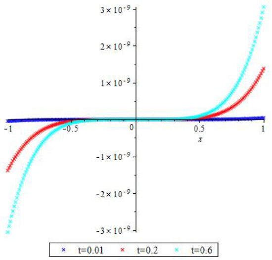
Figure 1.
Errors of Example 1, case (I).
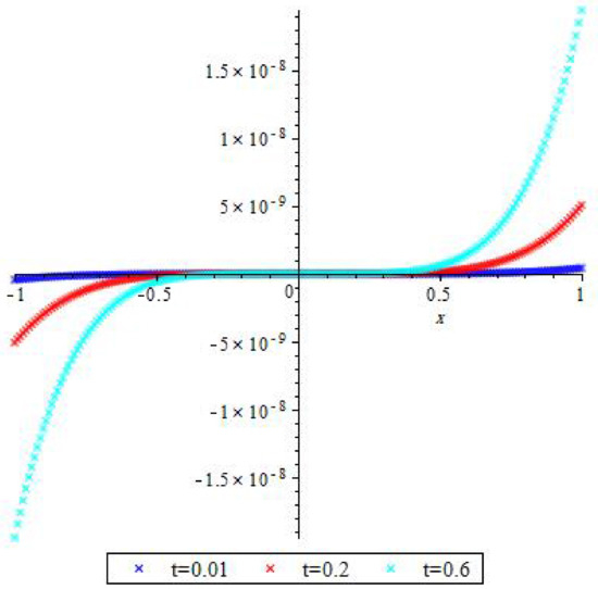
Figure 2.
Errors of Example 1, case (II).
From the above results, it is clear that the first case when the function of time for the known and unknown functions equal the results is better than the second case when the functions of the time for the known and unknown functions are different.
Note that choosing the time of the known function is the same as measuring the unknown function, resulting in less error and faster calculations. Therefore, in the following examples, we will apply this rule.
Example 2.
Consider the second-order MDeIDE:
under the conditions:
Comparing (27) with (1), then we have
First, separation of variables is applied for the MDeIDE (27), then we obtain the following FDeIDE:
Now, BPM can be applied to the FDeIDE (28) for different values of time and different values on
The approximate solutions for are given in the forms:
The approximate solutions for are given in the forms:
The approximate solution for are given in the forms:
The approximate solutions with different values of time presented in Figure 3, while the absolute errors of the MDeIDE (28) are presented in Table 2 and Table 3 and Figure 4, Figure 5, Figure 6, Figure 7, Figure 8 and Figure 9.
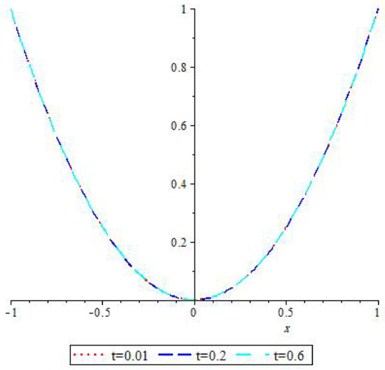
Figure 3.
Approximate solutions of Example 2, N = 5.
Table 2.
Absolute errors of Example 2, N = 5.
Table 3.
Absolute errors of Example 2, N = 6.
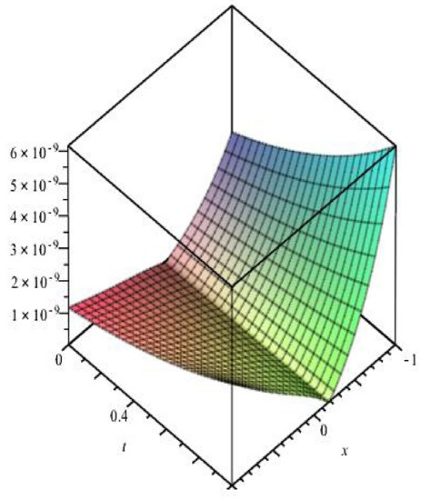
Figure 4.
Abs. error of Example 2, N = 5, t = 0.01.
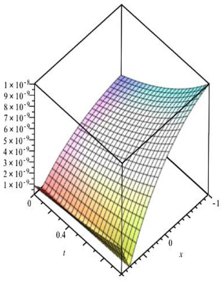
Figure 5.
Abs. error of Example 2, N = 5, = 0.2.
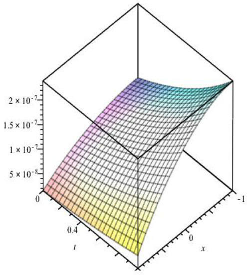
Figure 6.
Abs. error of Example 2, N = 5, t = 0.6.
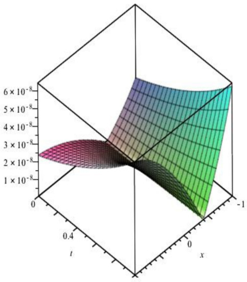
Figure 7.
Abs. error of Example 2, N = 6, t = 0.01.
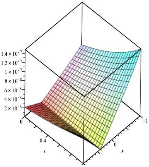
Figure 8.
Abs. error of Example 2, N = 6, t = 0.2.
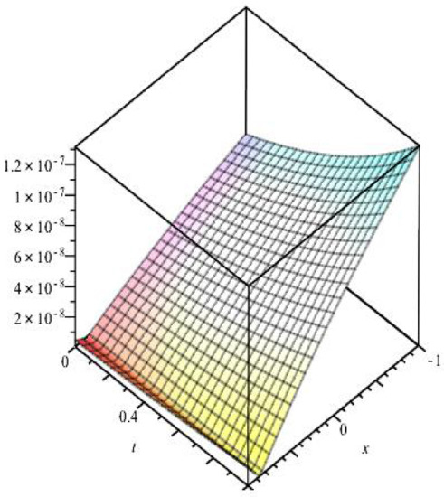
Figure 9.
Abs. error of Example 2, N = 6, t = 0.6.
In Example 2, we deduce that the integral operator of time is The corresponding errors with respect to the approximate solution for at different times , and are considered in Table 2). The approximate solutions for the same times , and and position divisions are computed in Figure 3. Figure 4 describes the arithmetic error at time , Figure 5 at time , and Figure 6 at time
In addition, for the same integral operator , Table 3 describes the arithmetic error for at different times (Figure 7), (Figure 8) and (Figure 9).
Example 3.
Consider the third-order MDeIDE:
under the conditions:
where
Applying separation of variables and BPM with different values of N and time, we obtain the approximate solutions in the following forms and Figure 10, while the absolute errors are presented in Table 4 and Table 5 and Figure 11, Figure 12, Figure 13, Figure 14, Figure 15 and Figure 16.
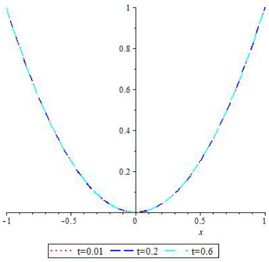
Figure 10.
Approximate solutions of Example 3, N = 6.
Table 4.
Absolute errors of Example 3, N = 5.
Table 5.
Absolute errors of Example 3, N = 6.
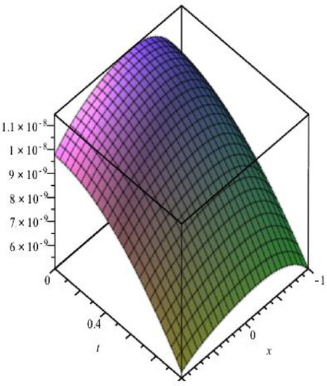
Figure 11.
Abs. error of Example 3, N = 5, t = 0.01.
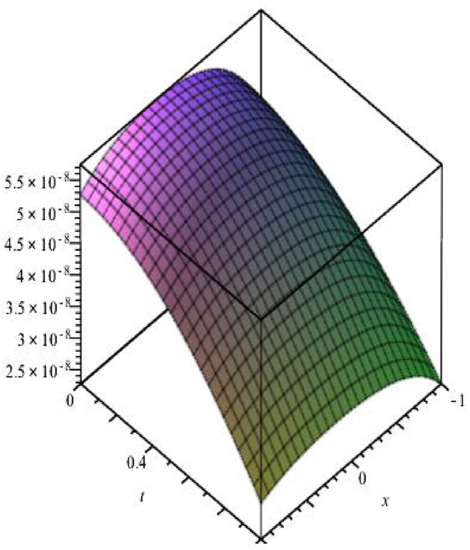
Figure 12.
Abs. error of Example 3, N = 5, t = 0.2.
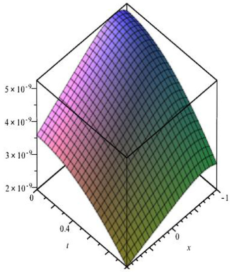
Figure 13.
Abs. error of Example 3, N = 5, t = 0.6.
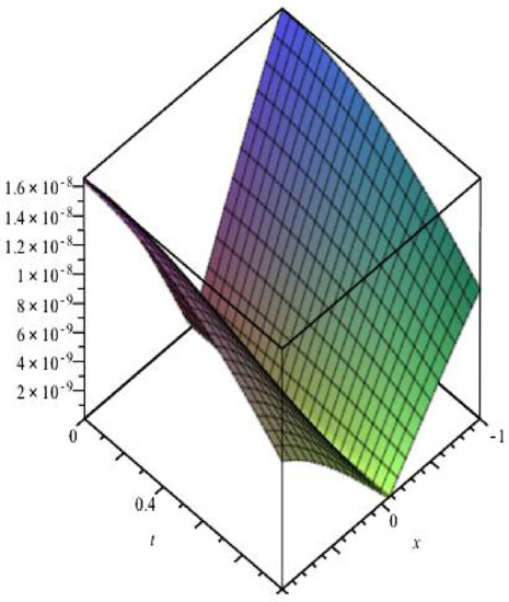
Figure 14.
Abs. error of Example 3, N = 6, t = 0.01.
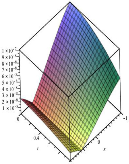
Figure 15.
Abs. error of Example 3, N = 6, t = 0.2.
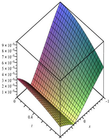
Figure 16.
Abs. error of Example 3, N = 6, t = 0.6.
In Example 3, the time integral operator is in the form . We compute the corresponding errors at and and position divisions are computed in Table 4 and Table 5, respectively. The approximate solutions corresponding to the same times and and position divisions are considered in Figure 10. Figure 11, Figure 12 and Figure 13 descript the error at , and and position divisions , respectively. In addition, Figure 14, Figure 15 and Figure 16 describe the error at , and and position divisions , respectively.
Example 4.
Consider the third-order MDeIDE:
under the conditions:
where
Similarly to Examples 1, 2, and 3, the approximate solutions of Equation (30), , and 5 are given by:
The approximate solution with different values of time presented in Figure 17, while the absolute errors are presented in Table 6, Table 7 and Table 8 and Figure 18, Figure 19, Figure 20, Figure 21, Figure 22, Figure 23, Figure 24 and Figure 25.
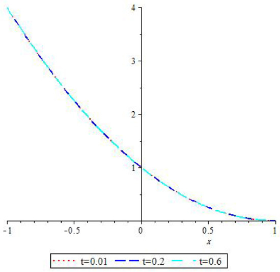
Figure 17.
Approximate solutions of Example 4, N = 5.
Table 6.
Absolute errors of Example 4, t = 0.01.
Table 7.
Absolute errors of Example 4, t = 0.2.
Table 8.
Absolute errors of Example 4, t = 0.6.
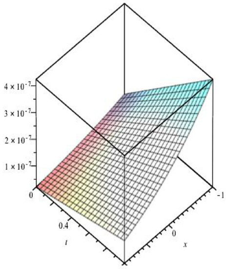
Figure 18.
Abs. error of Example 4, N = 4, t = 0.01.
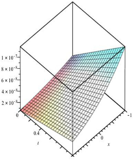
Figure 19.
Abs. error of Example 4, N = 5, t = 0.01.
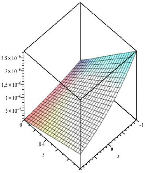
Figure 20.
Abs. error of Example 4, N = 3, t = 0.2.
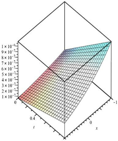
Figure 21.
Abs. error of Example 4, N = 4, t = 0.2.
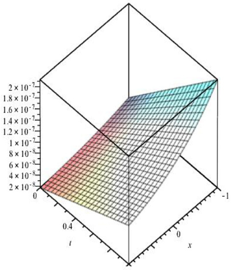
Figure 22.
Abs. error of Example 4, N = 5, t = 0.2.
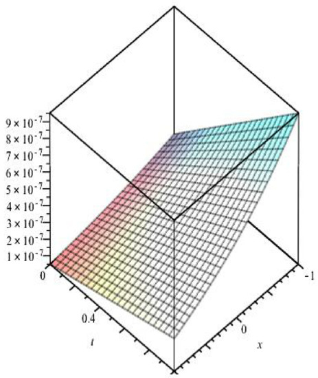
Figure 23.
Abs. error of Example 4, N = 3, t = 0.6.
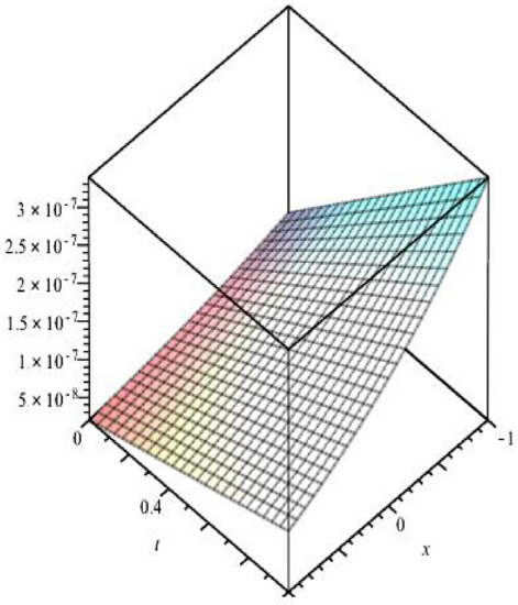
Figure 24.
Abs. error of Example 4, N = 4, t = 0.6.

Figure 25.
Abs. error of Example 4, N = 5, t = 0.6.
In Example 4, for and time The corresponding error for , and 5 are considered in Table 6, respectively, while for time and for , and 5, the arithmetic errors are computed in Table 7, respectively. The approximation solutions at , and and position divisions are computed at Figure 17, while Figure 18, Figure 19 and Figure 20 describe the arithmetic errors for ; and , respectively. Moreover, at see Figure 21, and at see Figure 22. At time , and see Figure 23, Figure 24 and Figure 25, respectively.
5. Conclusions
From the above results and discussion, we can establish the following:
- 1
- In the present article, the Bernoulli polynomial method with aid of separation of variables could be applied for solving (1+1) dimensional mixed-difference integro-differential equations with variable coefficients under mixed conditions.
- 2
- Four numerical examples are presented to illustrate the effectively of the method. The numerical results are presented in tables and figures. For example, Figure 3, Figure 10, and Figure 17 included the approximate solution of Examples 2, 3, and 4, respectively, for different values of time and N. Figure 1 and Figure 2, Figure 4, Figure 5, Figure 6, Figure 7, Figure 8 and Figure 9, Figure 11, Figure 12, Figure 13, Figure 14, Figure 15 and Figure 16, and Figure 18, Figure 19, Figure 20, Figure 21, Figure 22, Figure 23, Figure 24 and Figure 25 included the absolute errors of each example with different values of time.
- 3
- 4
- In the second example in Table 2 at the error is as high as possible at point and its value is . Furthermore, the error begins to decrease, and when the value of its value is It is also clear that the error ratio between the time rates at is This indicates that choosing the time function enabled the authors to adjust the error amount between the lowest time and the highest time by . This ratio is also measured at
- 5
- In the third example from Table 4, we find the following: time can be represented as a linear combination between polynomials and trigonometric functions. This helped to quasi-stabilize the error in , where we find the values of the arithmetic errors at are, respectively, , and Whereas, when the arithmetic errors are as follows: , and This continuous convergence in the error rate, whether at the lowest point and the highest point or at different times, confirms that the technique of separating the variables made can reduce the relative error by choosing the appropriate time function. Furthermore, we note that if the value of N increases, the error decreases; for example, in Table 4, when at the points , the errors equal , while in Table 5, when at the same points, the errors decrease by
- 6
- It is clear that BPM has an easy methodology and is incredibly simple for computer programming.
Author Contributions
Conceptualization, M.A.A.; Methodology, A.M.S.M., M.A.A. and D.S.M.; Software, A.M.S.M. and D.S.M.; Validation, D.S.M.; Formal analysis, A.M.S.M.; Resources, A.M.S.M. and M.A.A.; Data curation, D.S.M.; Writing—original draft, A.M.S.M., M.A.A. and D.S.M.; Writing—review & editing, A.M.S.M., M.A.A. and D.S.M.; Supervision, M.A.A. All authors developed the approach, completed the analysis, and wrote the manuscript. All authors read the final draft and gave their consent. All authors have read and agreed to the published version of the manuscript.
Funding
This research received no external funding.
Conflicts of Interest
This article’s initial draft beginning or appearance were not affected by any adverse situations.
Future Work
In the forthcoming future work, the authors will discuss two important points, namely: (a) This method can be extended for solving a (2+1) dimensional mixed-difference integro-differential equation; (b) The same equation can be studied when the nucleus of the locus is abnormal and takes a general form.
References
- Aghazadeh, N.; Khajehnasiri, A.A. Solving nonlinear two-dimensional Volterra integro-differential equations by block-pulse functions. Math. Sci. 2013, 7, 1–6. [Google Scholar] [CrossRef]
- Tari, A.; Shahmorad, S. Differential transform method for the system of two-dimensional nonlinear Volterra integro-differential equations. Comput. Math. Appl. 2011, 61, 2621–2629. [Google Scholar] [CrossRef][Green Version]
- Hussain, A.K.; Fadhel, F.S.; Rusli, N.; Yahya, Z.R. Iteration variational method for solving two-dimensional partial integro-differential equations. J. Phys. Conf. Ser. 2020, 1591, 012091. [Google Scholar] [CrossRef]
- Hamoud, A.A.; Mohammed, N.M.; Ghadle, K.P.; Dhondge, S.L. Solving integro-differential equations by using numerical techniques. Int. J. Appl. Eng. Res. 2019, 14, 3219–3225. [Google Scholar]
- Khajehnasiri, A.A. Numerical solution of nonlinear 2d Volterra-Fredholm integro-differential equations by two-dimensional triangular function. Int. J. Appl. Comput. Math. 2016, 2, 575–591. [Google Scholar] [CrossRef]
- Mirzaee, F.; Alipour, S.; Samadyar, N. A numerical approach for solving weakly singular partial integro-differential equations via two-dimensional-orthonormal Bernstein polynomials with the convergence analysis. Numer. Methods Partial. Differ. Equ. 2019, 35, 615–637. [Google Scholar] [CrossRef]
- Rivaz, A.; Jahan, S.; Yousefi, F. Two-dimensional Chebyshev polynomials for solving two-dimensional integro-differential equations. Çankaya Univ. J. Sci. Eng. 2015, 12, 1–11. [Google Scholar]
- Behzadi, S. The use of iterative methods to solve two-dimensional nonlinear Volterra-Fredholm integro-differential equations. Commun. Numer. Anal. 2012, 2012, 1–20. [Google Scholar] [CrossRef]
- Ahmed, S.A.; Elzaki, T.M. On the comparative study integro-differential equations using difference numerical methods. J. King Saud-Univ.- Sci. 2020, 32, 84–89. [Google Scholar] [CrossRef]
- Pandey, P.K. Numerical solution of linear Fredholm integro-differential equations by non-standard finite difference method. Appl. Appl. Math. Int. J. 2015, 10, 1019–1026. [Google Scholar]
- Zada, L.; Al-Hamami, M.; Nawaz, R.; Jehanzeb, S.; Morsy, A.; Abdel-Aty, A.; Nisar, K.S. A new approach for solving Fredholm integro-differential equations. Inf. Sci. Lett. 2021, 10, 407–415. [Google Scholar]
- Al-Bugami, A.M. Two-dimensional Fredholm integro-differential equation with singular kernel and its numerical solutions. Adv. Math. Phys. 2022, 2022, 2501947. [Google Scholar] [CrossRef]
- El-Borai, M.M.; Abdou, M.A.; Youssef, M.I.M. On Adomians decomposition method for solving nonlocal perturbed stochastic fractional integro-differential equations. Life Sci. J. 2013, 10, 550–555. [Google Scholar]
- Abdou, M.A.; Elsayed, M.A. Fractional integro differential equation and spectral relationships. Int. J. Comput. Sci. Technol. 2014, 137–139. [Google Scholar]
- Aboodh, K.S.; Farah, R.A.; Almardy, I.A.; ALmostafa, F.A. Solution of partial integro-differential equations by using aboodh and double aboodh transform methods. Glob. J. Pure Appl. Math. 2017, 13, 4347–4360. [Google Scholar]
- Al-Bugami, A.M. Nonlinear Fredholm integro-differential equation in two-dimensional and its numerical solutions. Aims Math. 2021, 6, 10383–10394. [Google Scholar] [CrossRef]
- Saadatmandia, A.; Dehghan, M. Numerical solution of the higher-order linear Fredholm integro-differential-difference equation with variable coefficients. Comput. Math. Appl. 2010, 59, 2996–3004. [Google Scholar] [CrossRef]
- Gülsu, M.; Öztürk, Y.; Sezer, M. A new collocation method for solution of mixed linear integro-differential-difference equations. Appl. Math. Comput. 2010, 216, 2183–2198. [Google Scholar] [CrossRef]
- Erdem, K.; Yalçinbaş, S.; Sezer, M. A Bernoulli polynomial approach with residual correction for solving mixed linear Fredholm integro-differential-difference equations. J. Differ. Equa. Appl. 2013, 19, 1619–1631. [Google Scholar] [CrossRef]
- Aslan, B.; Gurbuz, B.; Sezer, M. A new collocation method for solution of mixed linear integro-differential difference equations. New Trends Math. Sci. 2015, 3, 133–146. [Google Scholar]
- Mollaoglu, T.; Sezer, M. A numerical approach with residual error estimation for solution of high-order linear differential-difference equations by using Gegenbauer polynomials. CBU J. Sci. 2017, 13, 39–49. [Google Scholar]
- Gümgüm, S.; Sava aneril, N.; Kürkü, O.; Sezer, M. A numerical technique based on Lucas polynomials together with standard and Chebyshev-Lobatto collocation points for solving functional integro-differential equations involving variable delays. Sak. Univ. J. Sci. 2018, 22, 1659–1668. [Google Scholar] [CrossRef]
- Yavuz, M.; Özkol, I. Solutions of integro-differential difference equations via differential transform method. J. Sci. Eng. 2021, 18, 33–46. [Google Scholar]
- Doha, E.H.; Hafez, R.M.; Abdelkawy, M.A.; Ezz-eldien, S.S.; Taha, T.M.; Amin, A.Z.M.; EL-Kalaawy, A.A.; Baleanu, D. Composite Bernoulli-laguerre collocation method for a class of hyperbolic telegraph-type equations. Rom. Rep. Phys. 2017, 69, 119. [Google Scholar]
- Dascioglu, A.; Sezer, M. Bernoulli collocation method for high-order generalized pantograph equations. New Trends Math. Sci. 2015, 3, 96–109. [Google Scholar]
- Mirzaee, F. Bernoulli collocation method with residual correction for solving integral-algebraic equations. J. Linear Topol. Algebr. 2015, 4, 193–208. [Google Scholar]
- Hafez, R.M.; Doha, E.H.; Bhrawy, A.H.; Baleanu, D. Numerical solutions of two-dimensional mixed Volterra-Fredholm integral equations via Bernoulli collocation method. Rom. Phys. 2017, 62, 1–11. [Google Scholar]
- Toutounian, F.; Tohidi, E.; Shateyi, S. A Collocation method based on the Bernoulli operational matrix for solving high-order linear complex differential equations in a rectangular domain. Abstr. Appl. Anal. 2013, 2013, 823098. [Google Scholar] [CrossRef]
- Alalyani, A.; Abdou, M.A.; Basseem, M. On a solution of a third kind mixed integro-differential equation with singular kernel using orthogonal polynomial method. J. Appl. Math. 2023, 2023, 5163398. [Google Scholar] [CrossRef]
- Alsulaiman, R.E.; Abdou, M.A.; Youssef, E.M.; Taha, M. Solvability of a nonlinear integro-differential equation with fractional order using the Bernoulli matrix approach. Aims Math. 2023, 8, 7515–7534. [Google Scholar] [CrossRef]
- Jan, A.R. Numerical solution via a singular mixed integral equation in (2+1) dimensional. Appl. Math. Inf. Sci. 2022, 16, 871–882. [Google Scholar]
- Jan, A.R. An asymptotic model for solving mixed integral equation in position and time. J. Math. 2022, 2022, 8063971. [Google Scholar] [CrossRef]
- Mahdy, A.M.S.; Nagdy, A.S.; Hashem, K.M.; Mohamed, D.S. A computational technique for solving three-dimensional mixed Volterra-Fredholm integral equations. Fractal Fract. 2023, 7, 196. [Google Scholar]
- Mahdy, A.M.S.; Mohamed, D.S. Approximate solution of cauchy integral equations by using Lucas polynomials. Comput. Appl. Math. 2022, 41, 403. [Google Scholar] [CrossRef]
- Mahdy, A.M.S.; Shokry, D.; Lotfy, K. Chelyshkov polynomials strategy for solving 2-dimensional nonlinear Volterra integral equations of the first kind. Comput. Appl. Math. 2022, 41, 257. [Google Scholar] [CrossRef]
- Alhazmi, S.E.; Abdou, M.A. A physical phenomenon for the fractional nonlinear mixed integro-differential equation using a general discontinuous kernel. Fractal Fract. 2023, 7, 173. [Google Scholar] [CrossRef]
- Abdou, M.A. On asymptotic methods for Fredholm- Volterra integral equation of the second kind in contact problems. J. CAM 2003, 154, 431–446. [Google Scholar]
- Apostol, T.M. Introduction to Analytic Number Theory; Springer: New York, NY, USA, 1976. [Google Scholar]


Disclaimer/Publisher’s Note: The statements, opinions and data contained in all publications are solely those of the individual author(s) and contributor(s) and not of MDPI and/or the editor(s). MDPI and/or the editor(s) disclaim responsibility for any injury to people or property resulting from any ideas, methods, instructions or products referred to in the content. |
© 2023 by the authors. Licensee MDPI, Basel, Switzerland. This article is an open access article distributed under the terms and conditions of the Creative Commons Attribution (CC BY) license (https://creativecommons.org/licenses/by/4.0/).