Event-Triggered Extended Dissipativity Fuzzy Filter Design for Nonlinear Markovian Switching Systems against Deception Attacks

Abstract

This article is concerned with the adaptive-event-triggered filtering problem as it relates to a class of nonlinear discrete-time systems characterized by interval Type-2 fuzzy models. The system under investigation is susceptible to Markovian switching and deception attacks. It is proposed to implement an improved event-triggering mechanism to reduce the unnecessary signal transmissions on the communication channel and formulate the extended dissipativity specification to quantify the transient dynamics of filtering errors. By resorting to the linear matrix inequality approach and using the information on upper and lower membership functions, stochastic analysis establishes sufficient conditions for the existence of the desired filter, ensuring the mean-squared stability and extended dissipativity of the augmented filtering system. Further, an optimization-based algorithm (PSO) is proposed for computing filter gains at an optimal level of performance. The developed scheme was finally tested through experimental numerical illustrations based on a single-link robot arm and a lower limbs system.

1. Introduction, Notations, and Outline

Throughout this section, we outline the literature review, the notations, and the study objectives.

1.1. Bibliographic Review

Dynamical systems are frequently subject to random changes because of component failures, changes in subsystem interconnections, or environmental changes. These processes motivate researchers to examine and characterize Markovian jump systems (MJSs). A Markovian jump system is a stochastic hybrid system that has finite modes of operation, where jumps between modes are controlled by a Markov process. Several recent research studies have focused on MJSs, resulting in significant publications about fault tolerance, target tracking, manufacturing, networked control, and multi-agent systems [1,2,3,4,5,6]. Despite many successes in this research, most practical systems are highly nonlinear, so linear MJSs impose marked limitations in real-world applications. In addition to overcoming this drawback, the T-S fuzzy models have recently been applied to deal with nonlinear complex systems due to their effective approximation of smoothly nonlinear models [7,8,9,10,11]. In general, the T-S fuzzy system encompasses Type-1 and Type-2 fuzzy systems. Type-1 models typically have crisp membership functions, while Type-2 models are used to deal with parameter uncertainties by incorporating upper and lower membership functions [12,13,14,15].

On the other hand, networked control systems (NCSs) are a type of control system in which many components of the system are connected via shared communication networks, such as actuators, controllers, and sensors [16,17]. Under resource-constrained scenarios, such as information interactions between agents with limited communication resources, it is difficult for physical systems to obtain energy supplies in a dynamic environment. Hence, in designing a control strategy, it is important to consider economy and cost, and the above-mentioned features will inevitably be subject to some constraints. Two types of techniques are generally applied to address this issue. The first one is the intermittent control proposed in [18], wherein the control resource is designed to conserve energy in conjunction with the communication connection condition. The second approach is the event-triggered control, in which the gain or resource is selected when there is a relatively large error state between the sensor and the actuator. This technique is also considered an adequate method of addressing the energy constraints in communications networks. In recent years, the ETS has received considerable attention with numerous achievements that relate to ET $H_{\infty }$ control, ET fault detection, ET sliding-mode controller design, ET consensus control, and ET state estimation systems, as summarized in [19,20,21,22,23,24,25,26,27] and the references therein. Since communication networks are open and network resources are limited, studies on cyber security issues based on communication-saving regulations for NCSs are extremely important. In particular, deception attacks pose a significant threat to the normal operation of NCSs since they are continually introducing errors into the correct data [28,29,30]. It is generally adopted to evade detection mechanisms for which the error vectors are small or even offensive in nature, thus trying to destroy the working state of the system simply by accumulating errors. Due to the wide range of applications for parameter estimation, target tracking, as well as system monitoring, the filtering problem has attracted substantial research attention in the past few decades. Furthermore, there is no doubt that the Kalman filtering method is widely used in many filter design strategies for signal processing, control, and optimization [31,32,33]. In many practical cases, however, the Kalman filter does not always fulfil the requirement that the external noise is caused by white processes with known statistical properties. For input signals with non-statistical characteristics, the performance criteria can be used to compensate for the disadvantage of Kalman filtering. The filtering issue aims at developing filters that satisfy prescribed performance levels concerning the output error and disturbance input. It is noteworthy that several efficient filtering strategies have been proposed up to this point, including the $H_{\infty }$ filtering [19,34,35,36], passive/dissipative filtering [37,38,39], and peak-to-peak filtering [40,41]. In this paper, we were first motivated by the extended dissipativity performance, which has been introduced to deal with the $(Q,R,S)$-dissipative and $L_2-L_{\infty }$ filtering problem in a unified framework. Further, the quoted papers examined the extended dissipative performance, which can be converted into four different performances using different parameters [10,29,42].

As an attractive approach, the event-triggered method has been recently used to cope with the filtering problem for different classes of systems, and substantial research attention with some outstanding results can be found in [36,43,44]. To mention a few, a singular neural network with time-varying delays and Markovian jump parameters was investigated in [23] to deal with the event-triggered dissipative filtering problem. An event-triggered communication mechanism was employed by the authors of [24], for the design of piecewise fuzzy diagnostic observers for discrete-time TS fuzzy systems. As has been shown in previous studies, it has been found that the above-mentioned traditional event-triggered mechanisms can reduce communication resources and improve transmission effectiveness. However, these mechanisms are designed with constant thresholds that are not capable of adjusting themselves based on actual transmission conditions. This leads to the proposal of adaptive-event-triggered mechanisms (AETMs), in which the triggering threshold is dynamically adjusted during the operation of the system. There was an investigation in [28] of the design of $H_{\infty }$ filters for discrete-time networked systems with an adaptive-event-triggered mechanism and hybrid cyber-attacks. In [45], a new dynamic-event-triggered protocol was developed to address the problem of filtering for affine systems presented by the Takagi–Sugeno fuzzy model. In [20], an observer-based finite-time $H_{\infty }$ controller was designed to accommodate discrete-time-varying systems with adaptive-event-triggered mechanisms. Reference [35] addressed the problem of adaptive-event-triggered $H_{\infty }$ filtering for discrete-time-delayed neural networks with missing measurements that occur randomly. It can be noted that the adaptive law proposed in [46], which has a lower bound, might result in conservative conclusions. Additionally, the AETMs proposed by [47,48] each suffer from a singular problem and may degenerate into traditional periodic-time-triggered mechanisms, which may limit their application in practice. As a result of the above considerations, the motivation appears to be the development of a new AETM that is capable of improving the existing ones. Moreover, our involvement with IT-2 fuzzy systems was motivated by the fact that, unlike Type-1 TS fuzzy systems, they do not share the same membership functions with fuzzy filters or controllers. By doing so, we can overcome the network delay problem affecting the fuzzy filter’s membership functions when using the parallel distribution compensation (PDC) approach with the Type-1 T-S fuzzy systems.

1.2. Objective and Outline

We were inspired by the discussion above to pursue this study, which examines the event-triggered filter problem for a class of uncertain nonlinear systems that incorporate Markov jump switching:

(i)

As an alternative to existing filtering schemes developed for Type-1 fuzzy systems [34,38,49], this study proposes a novel filter design for Markovian jump interval Type-2 fuzzy systems that simultaneously consider an event-triggered communication scheme and a deception attack.

(ii)

This work introduces a novel adaptive-event-triggered communication scheme that improves the use of network resources as opposed to [50,51,52], which assumed the triggering parameters are constant. This mechanism was shown to alleviate network bandwidth and reduce system conservatism effectively by comparing it with other strategies [35,48,53,54].

(iii)

As described in [30,55], an improved matrix decoupling approach, which can be implemented by selecting some constants, provides greater flexibility when designing filters. This study, in contrast to previous studies, used a meta-heuristic technique based on PSO to identify the parameters accurately.

We illustrate our scheme with experimental numerical results on a single-link robot arm and an isokinetic rehabilitation system and verify the effectiveness of the proposed scheme by conducting a feasibility study. The paper is organized as follows. Section 2 introduces preliminary results in which the model and assumptions are presented, as well as the problem under study is identified. In Section 3, the main conclusions of the article are presented and derived. An optimization algorithm is presented in Section 4 for determining filter gains and for obtaining optimal performance levels. To illustrate the potential applications of the proposed scheme, as well as to validate its effectiveness, Section 5 presents the computational framework for this work and experimental numerical illustrations of the proposed methodology on a single-link robot arm and an isokinetic rehabilitation system. In Section 6, we discuss some of the findings and limitations of our proposal, as well as suggestions for further investigation.

1.3. Notations

Table 1. Abbreviations, acronyms, and notations used in the present document.

Symbol	Definition
$\mathbb{R}$	set of real numbers
n	dimension of the Euclidean space
$\mathit{X}\in {\mathbb{R}}^{n\times m}$	$n\times m$ real matrix
$\mathit{X}>0$	real symmetric positive definite matrix $\mathit{X}$
$\parallel \mathit{X}\parallel$	norm of the matrix $\mathit{X}$
${\mathit{X}}^{\top }$	transpose of the matrix $\mathit{X}$
$\mathrm{sym}\left(\mathit{X}\right)$	$\mathit{X}+{\mathit{X}}^{\top }$
*	term that is induced by symmetry of a matrix
${\lambda }_{\max }\left(\right)$	the maximal eigenvalue of a matrix
$\mathbb{E}$	mathematical expectation
${\pi }_{pq}=P(r_{k+1}=q|{\overline{r}}_k=p)$	transition probability from states p to q
r	number of if–then rules
${\overline{r}}_k$	discrete-time Markov process
LMI	linear matrix inequalities
MJS	Markovian jump systems
NCS	networked control systems
ET	event-triggered
T-S	Takagi–Sugeno
IT-2	interval Type-2

presents the abbreviations, acronyms, and notations used in this article.

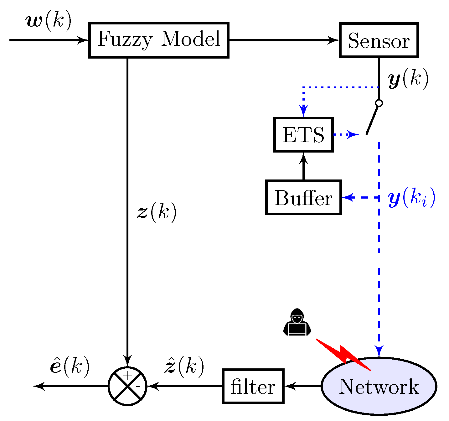
2. System Description and Problem Formulation

2.1. Markovian Jump T-S-Fuzzy-Model-Based NCS

Consider a class of nonlinear discrete-time Markovian jump systems, which can be expressed by the following fuzzy model on a complete probability space $(\mathsf{\Omega },\mathcal{F},\mathcal{P})$.

$$\begin{array}{cc}\hfill & {\mathbf{R}}_i:\mathrm{If}{\theta }_1\left(\mathit{x}\left(k\right)\right)\mathrm{is}{\mathit{M}}_i^1\mathrm{and}\mathrm{If}{\theta }_2\left(\mathit{x}\left(k\right)\right)\mathrm{is}{\mathit{M}}_i^2\cdots \mathrm{If}{\theta }_s\left(\mathit{x}\left(k\right)\right)\mathrm{is}{\mathit{M}}_i^s,\mathrm{Then}\hfill \\ \hfill & \left\{\begin{array}{cc}\hfill \mathit{x}(k+1)& ={\mathit{A}}_i\left({\overline{r}}_k\right)\mathit{x}\left(k\right)+{\mathit{B}}_{wi}\left({\overline{r}}_k\right)\left(k\right)\hfill \\ \hfill \mathit{y}\left(k\right)& ={\mathit{C}}_{2i}\left({\overline{r}}_k\right)\mathit{x}\left(k\right)\hfill \\ \hfill \mathit{z}\left(k\right)& ={\mathit{C}}_{1i}\left({\overline{r}}_k\right)\mathit{x}\left(k\right)+{\mathit{D}}_{1i}\left({\overline{r}}_k\right)\left(k\right)\hfill \end{array}\right.\hfill \end{array}$$

(1)

where $\mathbf{\theta }\left(k\right)=[{\theta }_1\left(\mathit{x}\left(k\right)\right),{\theta }_2\left(\mathit{x}\left(k\right)\right),\cdots ,{\theta }_s\left(\mathit{x}\left(k\right)\right)]$ are measurable premise variables of the system; ${\mathit{M}}_i^{\iota },\iota =1,2,\cdots ,s$ are Type-2 fuzzy sets; $i\in \mathbb{S}\triangleq \{1,2,\dots ,r\}$ is the number of rules. Vectors $\mathit{x}\left(k\right)\in {\mathbb{R}}^n$, $\mathit{y}\left(k\right)\in {\mathbb{R}}^{n_y}$, $\mathit{w}\left(k\right)\in {\mathbb{R}}^m$, and $\mathit{z}\left(k\right)\in {\mathbb{R}}^q$ define, respectively, the state, the output, the disturbance input, and the measured output. Matrices ${\mathit{A}}_i\left({\overline{r}}_k\right)$, ${\mathit{B}}_{wi}\left({\overline{r}}_k\right)$, ${\mathit{C}}_{1i}\left({\overline{r}}_k\right)$ ${\mathit{D}}_{1i}\left({\overline{r}}_k\right)$, and ${\mathit{C}}_{2i}\left({\overline{r}}_k\right)$ are known with appropriate dimensions. According to the i-th rule, the firing strength consists of the interval sets described as

$$\begin{array}{c}\hfill {\mathfrak{M}}_i=\left[\begin{array}{cc}{\underline{\mu }}_i\left(\mathit{x}\left(k\right)\right)& {\overline{\mu }}_i\left(\mathit{x}\left(k\right)\right)\end{array}\right],\end{array}$$

(2)

where

$${\underline{\mu }}_i\left(\mathit{x}\left(k\right)\right)=\prod _{\iota =1}^s{\underline{\omega }}_{{\mathit{M}}_i^{\iota }\left(\mathbf{\theta }\left(k\right)\right)}\ge 0,{\overline{\mu }}_i\left(\mathit{x}\left(k\right)\right)=\prod _{\iota =1}^s{\overline{\omega }}_{{\mathit{M}}_i^{\iota }\left(\mathbf{\theta }\left(k\right)\right)}\ge 0$$

$$\begin{array}{c}\hfill {\overline{\mu }}_i\left(\mathit{x}\left(k\right)\right)\ge {\underline{\mu }}_i\left(\mathit{x}\left(k\right)\right)\ge 0,{\overline{\omega }}_{{\mathit{M}}_i^{\iota }\left(\mathbf{\theta }\left(k\right)\right)}\ge {\underline{\omega }}_{{\mathit{M}}_i^{\iota }\left(\mathbf{\theta }\left(k\right)\right)}\ge 0\end{array}$$

(3)

As a result, the global fuzzy model can be inferred in the following manner:

$$\begin{array}{c}\hfill \left\{\begin{array}{cc}\mathit{x}(k+1)\hfill & {\displaystyle =\sum _{i=1}^r{\mu }_i\left(\mathit{x}\left(k\right)\right)\left({\mathit{A}}_i\left({\overline{r}}_k\right)\mathit{x}\left(k\right)+{\mathit{B}}_{wi}\left({\overline{r}}_k\right)\left(k\right)\right)}\hfill \\ \mathit{y}\left(k\right)\hfill & {\displaystyle =\sum _{i=1}^r{\mu }_i\left(\mathit{x}\left(k\right)\right)\left({\mathit{C}}_{2i}\left({\overline{r}}_k\right)\mathit{x}\left(k\right)\right)}\hfill \\ \mathit{z}\left(k\right)\hfill & {\displaystyle =\sum _{i=1}^r{\mu }_i\left(\mathit{x}\left(k\right)\right)\left({\mathit{C}}_{1i}\left({\overline{r}}_k\right)\mathit{x}\left(k\right)+{\mathit{D}}_{1i}\left({\overline{r}}_k\right)\left(k\right)\right)}\hfill \end{array}\right.\end{array}$$

(4)

The normalized membership function ${\mu }_i\left(\mathit{x}\left(k\right)\right)$ satisfies ${\displaystyle \sum _{i=1}^r}{\mu }_i\left(\mathit{x}\left(k\right)\right)=1$ and is defined as

$$\begin{array}{cc}\hfill & {\mu }_i\left(\mathit{x}\left(k\right)\right)={\displaystyle \frac{{\underline{\alpha }}_i\left(\mathit{x}\left(k\right)\right){\underline{\mu }}_i\left(\mathit{x}\left(k\right)\right)+{\overline{\alpha }}_i\left(\mathit{x}\left(k\right)\right){\overline{\mu }}_i\left(\mathit{x}\left(k\right)\right)}{{\displaystyle \sum _{i=1}^r}{\underline{\alpha }}_i\left(\mathit{x}\left(k\right)\right){\underline{\mu }}_i\left(\mathit{x}\left(k\right)\right)+{\overline{\alpha }}_i\left(\mathit{x}\left(k\right)\right){\overline{\mu }}_i\left(\mathit{x}\left(k\right)\right)}},\hfill \end{array}$$

The weighting coefficients ${\underline{\alpha }}_i\left(\mathit{x}\left(k\right)\right)$ and ${\overline{\alpha }}_i\left(\mathit{x}\left(k\right)\right)$ satisfy

$$\begin{array}{c}\hfill 0\le {\underline{\alpha }}_i\left(\mathit{x}\left(k\right)\right),{\overline{\alpha }}_i\left(\mathit{x}\left(k\right)\right)\le 1,{\underline{\alpha }}_i\left(\mathit{x}\left(k\right)\right)+{\overline{\alpha }}_i\left(\mathit{x}\left(k\right)\right)=1\end{array}$$

(5)

and are related to the uncertain parameters of the model. These nonlinear functions may not be known, but exist and satisfy (5). Stochastic process $\{{\overline{r}}_k,k\ge 0\}$ is a Markov chain taking values in a finite set $\mathbb{N}=\{1,\cdots ,N\}$ with transition probability $\mathsf{\Pi }=\left[{\pi }_{pq}\right]$ defined as ${\pi }_{pq}=Pr(\overline{r}(k+1)=q|{\overline{r}}_k=p)$ satisfying ${\pi }_{pq}\ge 0$ and ${\sum }_{q=1}^N{\pi }_{pq}=1$ for all $p,q\in \mathbb{N}$.

2.2. Event-Triggered Schemes

This paper assumed the measurement outputs are sent over communication channels and an event-triggered mechanism is implemented to conserve network resources and determine whether the latest sampled data packet can be transmitted to the filter system (see Figure 1). Event-triggered schemes are generally based on an event generator defined as a logic function that determines whether the sampled data should be transmitted or not. Accordingly, the event generator function is defined as follows:

$$\begin{array}{c}\hfill U(k,{\mathit{e}}_y\left(k\right))={\mathit{e}}_y^{\top }(k)\mathsf{\Theta }{\mathit{e}}_y\left(k\right)-\sigma \left(k\right){\mathit{y}}^{\top }(k)\mathsf{\Theta }\mathit{y}\left(k\right)\end{array}$$

(6)

where ${\mathit{e}}_y\left(k\right)=\mathit{y}\left(k\right)-\mathit{y}\left(k_i\right)$ is the output error, $\mathit{y}\left(k_i\right)$ is the previously transmitted data at time $k_i$, and $\sigma \left(k\right)$ is the event-triggered threshold. The current data transmitted depend on the following constraint:

$$\begin{array}{c}\hfill k_{i+1}=inf\{k\in \mathbb{N}|k>k_i,U(k,{\mathit{e}}_y\left(k\right))>0\}\end{array}$$

(7)

where $0\le k_0\le k_1\le \cdots k_i\le \cdots$ are the sequence of ET instances. $\sigma \left(k\right)$ in (6) can be adaptively adjusted based on the following adaptive law defined by $\mathsf{\Theta }>0$ such that

$$\begin{array}{c}\hfill \Delta \sigma \left(k\right)=\sigma (k+1)-\sigma \left(k\right)=-{\epsilon }_0{\sigma }^2\left(k\right){\mathit{e}}_y^{\top }(k)\mathsf{\Theta }{\mathit{e}}_y\left(k\right)\end{array}$$

(8)

where ${\epsilon }_0$ is a positive constant. When ${\epsilon }_0=0$ and $0<\sigma \left(k\right)<1$, it is clear that $\sigma \left(k\right)$ becomes a constant.

An important feature of networked control systems is network delay, which is caused by the limited bit rate of communication channels, the waiting period during which the packets are sent, or the propagation and processing of signals. As a result, $\tau \left(k\right)\in [0,{\tau }_M)$ was included in this paper, where ${\tau }_M$ is a positive integer. Based on the behavior of ZOH, $\overline{\mathit{y}}\left(k\right)$ holds the value of ${\mathit{y}}_{k_i}$ in the interval $[k_i+{\tau }_{k_i},k_{i+1}+{\tau }_{k_{i+1}})$. Thus, we have

$$\begin{array}{c}\hfill \overline{\mathit{y}}\left(k\right)={\mathit{y}}_{k_i},k\in [k_i+{\tau }_{k_i},k_{i+1}+{\tau }_{k_{i+1}})\end{array}$$

(9)

There are then two cases that need to be discussed:

Case 1 

    If $k_i+{\tau }_M+1>k_{i+1}+{\tau }_{k_{i+1}}-1$, we define $\tau \left(k\right)=k-k_i,k\in [k_i+{\tau }_{k_i},k_{i+1}+{\tau }_{k_{i+1}})$. It is obvious that ${\tau }_{k_i}\le \tau \left(k\right)\le (k_{i+1}-k_i)+{\tau }_{k_{i+1}}-1\le 1+{\tau }_M$.

Case 2 

     If $k_i+1+{\tau }_M<k_{i+1}+{\tau }_{k_{i+1}}$, we define the intervals $[k_i+{\tau }_{k_i},k_i+1+{\tau }_M),[k_i+{\tau }_M+j,k_i+{\tau }_M+j+1),(j=1,2,\cdots )$. Due to ${\tau }_{k_i}\le {\tau }_M$, there exists a positive integer $j^{*}$ such that

$$k_i+{\tau }_M+j^{*}<k_{i+1}+{\tau }_{k_{i+1}}<k_i+{\tau }_M+j^{*}+1$$

Hence, $\mathit{y}\left(k_i\right)$ and $\mathit{y}(k_i+j)$ with $j=1,2,\cdots ,j^{*}-1$ satisfy (7), and the time interval $[k_i+{\tau }_{k_i},k_{i+1}+{\tau }_{k_{i+1}})$ can be divided as

$$\begin{array}{c}\hfill [k_i+{\tau }_{k_i},k_{i+1}+{\tau }_{k_{i+1}})=\bigcup _{j=0}^{j^{*}}{\mathit{I}}_j\end{array}$$

(10)

where ${\mathit{I}}_0=[k_i+{\tau }_{k_i},k_i+{\tau }_M+1)$, ${\mathit{I}}_j=[k_i+{\tau }_M+j,k_i+{\tau }_M+j+1)$ and ${\mathit{I}}_{j^{*}}=[k_i+{\tau }_M+j^{*},k_{i+1}+{\tau }_{k_{i+1}})$. Define

$$\begin{array}{c}\hfill \tau \left(k\right)=\left\{\begin{array}{c}k-k_i,k\in {\mathit{I}}_0\hfill \\ k-k_i-j,k\in {\mathit{I}}_j\hfill \\ k-k_i-j^{*},k\in {\mathit{I}}_{j^{*}}\hfill \end{array}\right.\end{array}$$

Obviously, we obtain

$$\begin{array}{c}\hfill \left\{\begin{array}{c}{\tau }_{k_i}\le \tau \left(k\right)\le 1+{\tau }_M,k\in {\mathit{I}}_0\hfill \\ {\tau }_{k_i}\le {\tau }_M\le \tau \left(k\right)\le 1+{\tau }_M,k\in {\mathit{I}}_j\hfill \\ {\tau }_{k_i}\le {\tau }_M\le \tau \left(k\right)\le 1+{\tau }_M,k\in {\mathit{I}}_{j^{*}}\hfill \end{array}\right.\end{array}$$

Therefore, we have ${\tau }_m\le {\tau }_{k_i}\le \tau \left(k\right)\le {\tau }_M+1$, $k\in [k_i+{\tau }_{k_i},k_{i+1}+{\tau }_{k_{i+1}})$. In the first case, we define ${\mathit{e}}_y\left(k\right)=0$; in the second case, ${\mathit{e}}_y\left(k\right)$ is defined as

$$\begin{array}{c}\hfill {\mathit{e}}_y\left(k\right)=\left\{\begin{array}{c}0,k\in {\mathit{I}}_0\hfill \\ \mathit{y}\left(k_i\right)-\mathit{y}(k_i+j),k\in {\mathit{I}}_j\hfill \\ \mathit{y}\left(k_i\right)-\mathit{y}(k_i+j^{*}),k\in {\mathit{I}}_{j^{*}}\hfill \end{array}\right.\end{array}$$

Following the above discussion, the following relationship holds using (9):

$$\begin{array}{c}\hfill \overline{\mathit{y}}\left(k\right)={\mathit{y}}_{k_i}=\mathit{y}(k-\tau (k\left)\right)+{\mathit{e}}_y\left(k\right),k\in [k_i+{\tau }_{k_i},k_{i+1}+{\tau }_{k_{i+1}})\end{array}$$

(11)

Remark 1. 

It is important to point out that, to mitigate the communication burden and enhance the utilization of network resources, the adaptive-event-triggered mechanism is widely used in the analysis and design of networked systems [26,27,30]. Based on the above-mentioned literature, we adopted the adaptive-event-triggered mechanism (8) to investigate the filtering problem of Markov IT-2 fuzzy systems subject to cyber-attack.

In addition, according to (8), the event-triggered interval is greater than zero [56], which indicates that the proposed event-triggered transmission mechanism does not incorporate Zeno’s behavior.

2.3. Deception Attacks

Furthermore, this paper discusses networked T-S fuzzy systems with deception attacks. The open networked environment leads to the possibility of data being modified through deception attacks in a random manner, where a stochastic process is adopted to describe this scenario.

During deception attacks, transmitted data may take the following form:

$$\begin{array}{c}\hfill {\mathit{y}}_{\zeta }\left(k\right)=\overline{\mathit{y}}\left(k\right)+\zeta \left(k\right)(-\overline{\mathit{y}}\left(k\right))+\mathit{a}(\overline{\mathit{y}}\left(k\right))\end{array}$$

(12)

Here, $\zeta \left(k\right)$ represents the Bernoulli random variable that meets the following conditions:

$$Pr\{\zeta \left(k\right)=1\}=\overline{\zeta },Pr\{\zeta \left(k\right)=0\}=1-\overline{\zeta }$$

$\mathit{a}(\overline{\mathit{y}}\left(k\right))$ represents the embedded signal launched by the attacker. It was assumed that $\mathit{a}(\overline{\mathit{y}}\left(k\right))$ is a sufficiently smooth continuous nonlinear function satisfying the sector condition:

$$\begin{array}{cc}\hfill & \parallel \mathit{a}(\overline{\mathit{y}}\left(k\right))\parallel \le \parallel \mathit{G}\mathit{y}\left(k\right)\parallel \hfill \end{array}$$

(13)

where G is a known constant matrix.

2.4. Fuzzy Filter

To estimate the signal ${\mathit{z}}_k$ in Model (4), the following fuzzy filter is defined:

$$\begin{array}{cc}\hfill & {\mathbf{R}}_j:\mathrm{If}{\vartheta }_1\left(\widehat{\mathit{x}}\left(k\right)\right)\mathrm{is}{\mathcal{N}}_j^1\mathrm{and}\mathrm{If}{\vartheta }_2\left(\widehat{\mathit{x}}\left(k\right)\right)\mathrm{is}{\mathcal{N}}_j^2\cdots \mathrm{If}{\vartheta }_v\left(\widehat{\mathit{x}}\left(k\right)\right)\mathrm{is}{\mathcal{N}}_j^v,\mathrm{Then}\hfill \\ \hfill & \left\{\begin{array}{cc}\widehat{\mathit{x}}(k+1)\hfill & ={\widehat{\mathit{A}}}_j\left({\overline{r}}_k\right)\widehat{\mathit{x}}\left(k\right)+{\widehat{\mathit{B}}}_j\left({\overline{r}}_k\right){\mathit{y}}_{\zeta }\left(k\right)\hfill \\ \widehat{\mathit{z}}\left(k\right)\hfill & ={\widehat{\mathit{C}}}_j\left({\overline{r}}_k\right)\widehat{\mathit{x}}\left(k\right)\hfill \end{array}\right.\hfill \end{array}$$

where $\widehat{\mathit{x}}\left(k\right)$ is the filter state, $\widehat{\mathit{z}}\left(k\right)$ is the filter output, $\mathbf{\vartheta }\left(k\right)=[{\vartheta }_1\left(\widehat{\mathit{x}}\left(k\right)\right),{\vartheta }_2\left(\widehat{\mathit{x}}\left(k\right)\right),\dots ,{\vartheta }_v\left(\widehat{\mathit{x}}\left(k\right)\right)]$ are the premise variables, and ${\mathcal{N}}_j^{\varsigma },\varsigma =1,2,\cdots ,v$ stands for the Type-2 fuzzy sets of the filter; ${\widehat{\mathit{A}}}_j\left({\overline{r}}_k\right)$, ${\widehat{\mathit{B}}}_j\left({\overline{r}}_k\right)$ and ${\widehat{\mathit{C}}}_j\left({\overline{r}}_k\right)$ are unknown matrices that should be designed.

$$\begin{array}{c}\hfill {\mathfrak{N}}_j=\left[\begin{array}{cc}{\underline{\nu }}_j\left(\widehat{\mathit{x}}\left(k\right)\right)& {\overline{\nu }}_j\left(\widehat{\mathit{x}}\left(k\right)\right)\end{array}\right],\end{array}$$

(14)

where

$${\underline{\nu }}_j\left(\widehat{\mathit{x}}\left(k\right)\right)=\prod _{\varsigma =1}^v{\underline{\omega }}_{{\mathcal{N}}_j^{\varsigma }\left(\mathbf{\vartheta }\left(k\right)\right)}\ge 0,{\overline{\nu }}_j\left(\widehat{\mathit{x}}\left(k\right)\right)=\prod _{\varsigma =1}^v{\overline{\omega }}_{{\mathcal{N}}_j^{\varsigma }\left(\mathbf{\vartheta }\left(k\right)\right)}\ge 0$$

$$\begin{array}{c}\hfill {\underline{\nu }}_j\left(\widehat{\mathit{x}}\left(k\right)\right)\ge {\overline{\nu }}_j\left(\widehat{\mathit{x}}\left(k\right)\right)\ge 0,{\overline{\omega }}_{{\mathcal{N}}_j^{\varsigma }\left(\mathbf{\vartheta }\left(k\right)\right)}\ge {\underline{\omega }}_{{\mathcal{N}}_j^{\varsigma }\left(\mathbf{\vartheta }\left(k\right)\right)}\ge 0\end{array}$$

(15)

The global fuzzy filter is defined as follows:

$$\begin{array}{c}\hfill \left\{\begin{array}{cc}\widehat{\mathit{x}}(k+1)\hfill & {\displaystyle =\sum _{j=1}^r{\nu }_j\left(\widehat{\mathit{x}}\left(k\right)\right)({\widehat{\mathit{A}}}_j\left({\overline{r}}_k\right)\widehat{\mathit{x}}\left(k\right)+{\widehat{\mathit{B}}}_j\left({\overline{r}}_k\right){\mathit{y}}_{\zeta }\left(k\right))}\hfill \\ \widehat{\mathit{z}}\left(k\right)\hfill & {\displaystyle =\sum _{j=1}^r{\nu }_j\left(\widehat{\mathit{x}}\left(k\right)\right)\left({\widehat{\mathit{C}}}_j\left({\overline{r}}_k\right)\widehat{\mathit{x}}\left(k\right)\right)}\hfill \end{array}\right.\end{array}$$

(16)

$$\begin{array}{cc}\hfill & {\nu }_j\left(\widehat{\mathit{x}}\left(k\right)\right)={\displaystyle \frac{{\underline{\beta }}_j\left(\widehat{\mathit{x}}\left(k\right)\right){\underline{\nu }}_j\left(\widehat{\mathit{x}}\left(k\right)\right)+{\overline{\beta }}_j\left(\widehat{\mathit{x}}\left(k\right)\right){\overline{\nu }}_j\left(\widehat{\mathit{x}}\left(k\right)\right)}{{\displaystyle \sum _{l=1}^r({\underline{\beta }}_l\left(\widehat{\mathit{x}}\left(k\right)\right){\underline{\nu }}_l\left(\widehat{\mathit{x}}\left(k\right)\right)+{\overline{\beta }}_l\left(\widehat{\mathit{x}}\left(k\right)\right){\overline{\nu }}_l\left(\widehat{\mathit{x}}\left(k\right)\right))}}},{\nu }_j\left(\widehat{\mathit{x}}\left(k\right)\right)\ge 0,\sum _{j=1}^r{\nu }_j\left(\widehat{\mathit{x}}\left(k\right)\right)=1\hfill \end{array}$$

(17)

The two nonlinear functions ${\underline{\beta }}_j\left(\widehat{\mathit{x}}\left(k\right)\right)$ and ${\overline{\beta }}_j\left(\widehat{\mathit{x}}\left(k\right)\right)$ satisfy

$$\begin{array}{c}\hfill 0\le {\underline{\beta }}_j\left(\widehat{\mathit{x}}\left(k\right)\right),{\overline{\beta }}_j\left(\widehat{\mathit{x}}\left(k\right)\right)\le 1,{\underline{\beta }}_j\left(\widehat{\mathit{x}}\left(k\right)\right)+{\overline{\beta }}_j\left(\widehat{\mathit{x}}\left(k\right)\right)=1\end{array}$$

(18)

For simplicity, in the sequel, ${\mu }_i\left(\mathit{x}\left(k\right)\right)$ and ${\nu }_j\left(\widehat{\mathit{x}}\left(k\right)\right)$ are denoted as ${\mu }_i$ and ${\widehat{\nu }}_j$, respectively.

Let $\widehat{\mathit{e}}\left(k\right)=\mathit{z}\left(k\right)-\widehat{\mathit{z}}\left(k\right)$. Taking (4) and (16) together, we can represent the filtering error system as follows:

$$\begin{array}{c}\hfill \left\{\begin{array}{cc}\tilde{\mathit{x}}(k+1)\hfill & {\displaystyle =\sum _{i=1}^r\sum _{j=1}^r{\mu }_i{\widehat{\nu }}_j({\tilde{\mathit{A}}}_{ij}^p\tilde{\mathit{x}}\left(k\right)+(1-\overline{\zeta }){\tilde{\mathit{A}}}_{dij}^p\tilde{\mathit{x}}(k-\tau \left(k\right))+(1-\overline{\zeta }){\tilde{\mathit{B}}}_{ej}^p{\mathit{e}}_y\left(k\right)}\hfill \\ & +\overline{\zeta }{\tilde{\mathit{B}}}_{ej}^p\mathit{a}(\overline{\mathit{y}}\left(k\right))+{\tilde{\mathit{B}}}_{1i}^p\mathit{w}\left(k\right)+(\zeta \left(k\right)-\overline{\zeta }){\tilde{\mathit{B}}}_g\mathit{g}\left(\tilde{\mathit{x}}\left(k\right)\right))\hfill \\ \widehat{\mathit{e}}\left(k\right)\hfill & {\displaystyle =\sum _{i=1}^r\sum _{j=1}^r{\mu }_i{\widehat{\nu }}_j\left({\tilde{\mathit{C}}}_{ij}^p\tilde{\mathit{x}}\left(k\right)+{\tilde{\mathit{D}}}_i^p\mathit{w}\left(k\right)\right)}\hfill \end{array}\right.\end{array}$$

(19)

where $\tilde{\mathit{x}}\left(k\right)={\left[{\mathit{x}}^{\top }\left(k\right),{\widehat{\mathit{x}}}^{\top }\left(k\right)\right]}^{\top }$ ${\tilde{\mathit{A}}}_{ij}^p=\left[\begin{array}{cc}{\mathit{A}}_i^p& \mathbf{0}\\ \mathbf{0}& {\widehat{\mathit{A}}}_j^p\end{array}\right]$$,{\tilde{\mathit{A}}}_{dij}^p=\left[\begin{array}{cc}\mathbf{0}& \mathbf{0}\\ {\widehat{\mathit{B}}}_j^p{\mathit{C}}_{2i}^p& \mathbf{0}\end{array}\right]$, ${\tilde{\mathit{B}}}_{ej}^p=\left[\begin{array}{c}\mathbf{0}\\ {\widehat{\mathit{B}}}_j^p\end{array}\right]$, ${\tilde{\mathit{B}}}_{1i}^p=\left[\begin{array}{c}{\mathit{B}}_{1i}^p\\ \mathbf{0}\end{array}\right]$, ${\tilde{\mathit{B}}}_g=\left[\begin{array}{c}\mathbf{0}\\ \mathit{I}\end{array}\right]$, ${\tilde{\mathit{C}}}_{ij}^p=\left[\begin{array}{cc}{\mathit{C}}_{1i}^p& -{\widehat{\mathit{C}}}_j^p\end{array}\right]$, ${\tilde{\mathit{D}}}_i^p={\mathit{D}}_{1i}^p$, $\mathit{g}\left(\tilde{\mathit{x}}\left(k\right)\right)={\widehat{\mathit{B}}}_j^p\left(\mathit{a}\right(\overline{\mathit{y}}\left(k\right))-{\mathit{C}}_{2i}^p\mathit{x}(k-\tau \left(k\right))-{\mathit{e}}_y\left(k\right))$.

2.5. Problem Formulation

Based on the above description, the objective of this article is to design the parameters of Filter (16) such that System (19) is asymptotically mean-squared stable with extended dissipative performance, i.e.:

1.

System (19) is mean-squared stable;

2.

Under zero initial conditions, the following criterion holds for $\mathit{w}\left(k\right)\ne \mathbf{0}$:

$$\mathbb{E}\left\{\sum _{k=0}^{K_f}J\left(k\right)\right\}\ge \underset{0\le k\le K_f}{sup}\mathbb{E}\left\{{\widehat{\mathit{e}}}^{\top }(k){\mathsf{\Omega }}_4\widehat{\mathit{e}}\left(k\right)\right\}$$

(20)

where $J\left(k\right)={\widehat{\mathit{e}}}^{\top }\left(k\right){\mathsf{\Omega }}_1\widehat{\mathit{e}}\left(k\right)+2{\widehat{\mathit{e}}}^{\top }\left(k\right){\mathsf{\Omega }}_2\mathit{w}\left(k\right)+{\mathit{w}}^{\top }\left(k\right){\mathsf{\Omega }}_3\mathit{w}\left(k\right)$, and matrices ${\mathsf{\Omega }}_1$, ${\mathsf{\Omega }}_2$, ${\mathsf{\Omega }}_3$ and ${\mathsf{\Omega }}_4$ satisfy the following assumption:

Assumption 1 

([57]). For known real matrices ${\mathsf{\Omega }}_1={\mathsf{\Omega }}_1\le 0$, ${\mathsf{\Omega }}_2$, ${\mathsf{\Omega }}_3={\mathsf{\Omega }}_3^{\top }\ge 0$, and ${\mathsf{\Omega }}_4={\mathsf{\Omega }}_{\top }^4={\left({\mathsf{\Omega }}_4^{+}\right)}^{\top }{\mathsf{\Omega }}_4^{+}\ge 0$, it was assumed that:

(i) 

$\Vert {\mathit{D}}_i^p\Vert \Vert {\mathsf{\Omega }}_4\Vert =0$;

(ii) 

$(\Vert {\mathsf{\Omega }}_1\Vert +\Vert {\mathsf{\Omega }}_2\Vert )\Vert {\mathsf{\Omega }}_4\Vert =0$.

Remark 2. 

From (20), the extended dissipativity criterion includes $H_{\infty }$, strict dissipativity, $l_2-l_{\infty }$, or passivity performances as special cases according to the different values of the matrices:

-

If ${\mathsf{\Omega }}_1=-\mathit{I}$, ${\mathsf{\Omega }}_2=0$, ${\mathsf{\Omega }}_3={\gamma }^2\mathit{I}$, and ${\mathsf{\Omega }}_4=\mathbf{0}$, Inequality (20) reduces to an $H_{\infty }$ performance requirement.

-

If ${\mathsf{\Omega }}_3=\mathit{R}-\mathit{I}\gamma$$(\gamma >\mathbf{0})$ and ${\mathsf{\Omega }}_4=0$, Inequality (20) corresponds to a strict dissipativity.

-

If ${\mathsf{\Omega }}_1=\mathbf{0}$, ${\mathsf{\Omega }}_2=\mathbf{0}$, ${\mathsf{\Omega }}_3={\gamma }^2\mathit{I}$, and ${\mathsf{\Omega }}_4=\mathit{I}$, Inequality (20) reduces to an $l_2-l_{\infty }$ performance.

-

If $\widehat{\mathit{e}}\left(k\right)$ and $\mathit{w}\left(k\right)$ have the same dimension and ${\mathsf{\Omega }}_1=\mathbf{0}$, ${\mathsf{\Omega }}_2=\mathit{I}$, ${\mathsf{\Omega }}_3=\gamma \mathit{I}$, and ${\mathsf{\Omega }}_4=\mathbf{0}$, the passivity will be obtained.

Next, we present some preliminaries that are crucial for the derivation of our major conclusions.

Definition 1 

([58]). The filtering error system (19) is said to be stochastically mean-squared stable if the following condition holds:

$$\mathbb{E}\left\{\sum _{k=0}^{\infty }\Vert {\tilde{\mathit{x}}\left(k\right)}^2\Vert |(\tilde{\mathit{x}}\left(k_0\right),{\overline{r}}_0)\right\}<\infty$$

for any initial condition $(\tilde{\mathit{x}}\left(k_0\right),{\overline{r}}_0)$.

Lemma 1 

([59]). For given positive integers ${\tau }_m$ and ${\tau }_M$, a positive matrix Z, symmetric matrices, ${\mathit{Y}}_{11}$ and ${\mathit{Y}}_{22}$, and matrices ${\mathit{Y}}_{12}$, ${\mathit{T}}_1$, and ${\mathit{T}}_2$, such that

$$\begin{array}{c}\hfill \left[\begin{array}{ccc}{\mathit{Y}}_{11}& {\mathit{Y}}_{12}& {\mathit{T}}_1\\ *& {\mathit{Y}}_{22}& {\mathit{T}}_2\\ *& *& \mathit{Z}\end{array}\right]\ge 0\end{array}$$

(21)

the following inequality holds:

$$\begin{array}{cc}\hfill -\sum _{s=k-{\tau }_M}^{k-{\tau }_m-1}{\mathbf{\eta }}^{\top }\left(s\right)\mathit{Z}\mathbf{\eta }\left(s\right)& \le {\mathbf{\psi }}^{\top }\left(k\right)\left({\tau }_r({\mathit{Y}}_{11}+{\displaystyle \frac{1}{3}}{\mathit{Y}}_{22})+\mathit{sym}\{{\mathit{T}}_1{\mathit{e}}_{12}+{\mathit{T}}_2{\mathit{e}}_{123}\}\right)\mathbf{\psi }\left(k\right)\hfill \end{array}$$

where ${\tau }_r={\tau }_M-{\tau }_m\ge 1$, $\mathbf{\eta }\left(k\right)=\mathit{x}(k+1)-\mathit{x}\left(k\right)$, and $\mathbf{\psi }\left(k\right)=\left[{\mathit{x}}^{\top }\right(k-{\tau }_m){\mathit{x}}^{\top }(k-{\tau }_M){\frac{1}{{\tau }_r+1}{\sum }_{s=k-{\tau }_M}^{k-{\tau }_m-1}{\mathit{x}}^{\top }\left(s\right)]}^{\top }$, ${\mathit{e}}_{12}=[\mathit{I}-\mathit{I}\mathbf{0}],$ and ${\mathit{e}}_{123}=[\mathit{I}\mathit{I}-2\mathit{I}]$.

3. Main Results

3.1. Extended Dissipative Analysis

This section concerns the derivation of sufficient conditions in such a way that the filtering error system (19) is stochastically mean-squared stable with extended dissipativity performance.

Theorem 1. 

Consider the Markovian jump IT-2 fuzzy system (4) and Filter (16). For given matrices $\mathsf{\Theta }>0$, ${\mathsf{\Omega }}_1$, ${\mathsf{\Omega }}_2$, ${\mathsf{\Omega }}_3$, and ${\mathsf{\Omega }}_4$ satisfying Assumption 1 and positive scalars ${\varrho }_s$, if matrices ${\mathit{P}}^p$, ${\mathit{Q}}_v,v=1,2,3$, ${\mathit{Z}}_s$, ${\mathit{X}}_{1s}$, ${\mathit{Y}}_{1s}$, ${\mathit{Z}}_{1s}$, ${\mathit{T}}_{1s}$, ${\mathit{T}}_{2s}$, ${\mathit{T}}_{3s}$, ${\mathit{F}}_s^p$, and $s=1,2$ and scalars $\tau >0$ and ${\sigma }_0>1$ exist such that the following conditions hold:

  

$$\begin{array}{cc}\hfill & \left[\begin{array}{ccc}{\mathit{X}}_{11}& {\mathit{X}}_{12}& {\mathit{T}}_{11}\\ *& {\mathit{X}}_{22}& {\mathit{T}}_{12}\\ *& *& {\mathit{Z}}_1\end{array}\right]>0\left[\begin{array}{ccc}{\mathit{Y}}_{11}& {\mathit{Y}}_{12}& {\mathit{T}}_{21}\\ *& {\mathit{Y}}_{22}& {\mathit{T}}_{22}\\ *& *& {\mathit{Z}}_2\end{array}\right]>0\left[\begin{array}{ccc}{\mathit{Z}}_{11}& {\mathit{Z}}_{12}& {\mathit{T}}_{13}\\ *& {\mathit{Z}}_{22}& {\mathit{T}}_{23}\\ *& *& {\mathit{Z}}_2\end{array}\right]>0\hfill \end{array}$$

(22)

$$\begin{array}{cc}\hfill & \left[\begin{array}{cc}-{\mathit{P}}^p& {\left({\tilde{\mathit{C}}}_{ij}^p\right)}^{\top }{\left({\mathsf{\Omega }}_4^{+}\right)}^{\top }\\ *& -\mathit{I}\end{array}\right]<0\hfill \end{array}$$

(23)

$$\begin{array}{cc}\hfill & \left\{\begin{array}{cc}\hfill & {\tilde{\mathsf{\Phi }}}_{ii}^p<0\hfill \\ \hfill & {\tilde{\mathsf{\Phi }}}_{ij}^p+{\varrho }_1{\tilde{\mathsf{\Phi }}}_{ji}^p<0\hfill \\ \hfill & {\tilde{\mathsf{\Phi }}}_{ij}^p+{\varrho }_2{\tilde{\mathsf{\Phi }}}_{ji}^p<0,1\le i<j\le r\hfill \end{array}\right.\hfill \end{array}$$

(24)

then, System (19) is stochastically mean-squared stable and extended dissipative. The remaining matrices are defined as

$$\begin{array}{c}\hfill \begin{array}{cc}\hfill {\tilde{\mathsf{\Phi }}}_{ij}^p& =\left[\begin{array}{ccc}{\tilde{\mathsf{\Psi }}}_{ij}^p+{\widehat{\mathsf{\Psi }}}^p& {\left({\tilde{\mathcal{B}}}_{ij}^p\right)}^{\top }-{\left({\tilde{\mathcal{C}}}_{ij}^p\right)}^{\top }{\mathsf{\Omega }}_2& {\left({\tilde{\mathcal{C}}}_{ij}^p\right)}^{\top }\sqrt{-{\mathsf{\Omega }}_1}\\ *& -sym\left\{{\left({\tilde{\mathit{D}}}_i^p\right)}^{\top }{\mathsf{\Omega }}_2\right\}-{\mathsf{\Omega }}_3& {\left({\tilde{\mathit{D}}}_i^p\right)}^{\top }\sqrt{-{\mathsf{\Omega }}_1}\\ *& *& -\mathit{I}\end{array}\right]\hfill \\ \hfill {\tilde{\mathsf{\Psi }}}_{ij}^p& =\left[\begin{array}{cccccccccc}{\tilde{\mathsf{\Psi }}}_{11ij}^p& \mathbf{0}& (1-\overline{\zeta }){\mathit{F}}_1^p{\tilde{\mathit{A}}}_{dij}^p& \mathbf{0}& \mathbf{0}& \mathbf{0}& \mathbf{0}& {\tilde{\mathsf{\Psi }}}_{18ij}^p& (1-\overline{\zeta }){\mathit{F}}_1^p{\tilde{\mathit{B}}}_{ej}^p& \overline{\zeta }{\mathit{F}}_1^p{\tilde{\mathit{B}}}_{ej}^p\\ *& -{\mathit{Q}}_1& \mathbf{0}& \mathbf{0}& \mathbf{0}& \mathbf{0}& \mathbf{0}& \mathbf{0}& \mathbf{0}& \mathbf{0}\\ *& *& {\tilde{\mathsf{\Psi }}}_{33}^p& \mathbf{0}& \mathbf{0}& \mathbf{0}& \mathbf{0}& (1-\overline{\zeta }){\left({\mathit{F}}_2^p{\tilde{\mathit{A}}}_{dij}^p\right)}^{\top }& {\left({\mathit{C}}_{2i}^p\right)}^{\top }\mathsf{\Theta }& \mathbf{0}\\ *& *& *& -{\mathit{Q}}_2& \mathbf{0}& \mathbf{0}& \mathbf{0}& \mathbf{0}& \mathbf{0}& \mathbf{0}\\ *& *& *& *& \mathbf{0}& \mathbf{0}& \mathbf{0}& \mathbf{0}& \mathbf{0}& \mathbf{0}\\ *& *& *& *& *& \mathbf{0}& \mathbf{0}& \mathbf{0}& \mathbf{0}& \mathbf{0}\\ *& *& *& *& *& *& \mathbf{0}& \mathbf{0}& \mathbf{0}& \mathbf{0}\\ *& *& *& *& *& *& *& {\tilde{\mathsf{\Psi }}}_{88}^p& (1-\overline{\zeta }){\mathit{F}}_2^p{\tilde{\mathit{B}}}_{ej}^p& \overline{\zeta }{\mathit{F}}_1^p{\tilde{\mathit{B}}}_{ej}^p\\ *& *& *& *& *& *& *& *& (1-{\sigma }_0)& \mathbf{0}\\ *& *& *& *& *& *& *& *& *& -\tau \mathit{I}\end{array}\right]\hfill \\ \hfill {\tilde{\mathcal{B}}}_{ij}^p& =\left[\begin{array}{cccccccccc}{\left({\mathit{F}}_1^p{\tilde{\mathit{B}}}_{1i}^p\right)}^{\top }& \mathbf{0}& \mathbf{0}& \mathbf{0}& \mathbf{0}& \mathbf{0}& \mathbf{0}& {\left({\mathit{F}}_2^p{\tilde{\mathit{B}}}_{1i}^p\right)}^{\top }& \mathbf{0}& \mathbf{0}\end{array}\right]\hfill \\ \hfill {\tilde{\mathcal{C}}}_{ij}^p& =\left[\begin{array}{ccccccccccc}{\tilde{\mathit{C}}}_{ij}^p& \mathbf{0}& \mathbf{0}& \mathbf{0}& \mathbf{0}& \mathbf{0}& \mathbf{0}& \mathbf{0}& \mathbf{0}& \mathbf{0}& \mathbf{0}\end{array}\right],{\mathit{X}}_{}^p=\sum _{q=1}^N{\pi }_{pq}{\mathit{P}}_{}^q\hfill \\ \hfill {\tilde{\mathsf{\Psi }}}_{11ij}^p& =sym\left({\mathit{F}}_1^p({\tilde{\mathit{A}}}_{ij}^p-\mathit{I})\right)+({\mathit{X}}_{}^p-{\mathit{P}}^p)+{\mathit{Q}}_1+{\mathit{Q}}_2+({\tau }_r+1){\mathit{Q}}_3\hfill \\ \hfill {\tilde{\mathsf{\Psi }}}_{33}^p& =-{\mathit{Q}}_3+{\left({\mathit{C}}_{2i}^p\right)}^{\top }\mathsf{\Theta }{\mathit{C}}_{2i}^p+{\left({\mathit{C}}_{2i}^p\right)}^{\top }{\mathit{G}}^{\top }\mathit{G}{\mathit{C}}_{2i}^p,{\tilde{\mathsf{\Psi }}}_{18ij}^p=-{\mathit{F}}_1^p+{\mathit{X}}_{}^p+{\left({\mathit{F}}_2^p({\tilde{\mathit{A}}}_{ij}^p-\mathit{I})\right)}^{\top }\hfill \\ \hfill {\tilde{\mathsf{\Psi }}}_{88}^p& =-\mathit{sym}\left({\mathit{F}}_2^p\right)+{\mathit{X}}_{}^p+{\tau }_m{\mathit{Z}}_1+{\tau }_r{\mathit{Z}}_2\hfill \\ \hfill {\tilde{\mathsf{\Psi }}}^p& ={\mathsf{\Pi }}_1^{\top }\left({\tau }_m({\mathit{X}}_{11}+{\displaystyle \frac{1}{3}}{\mathit{X}}_{22})+\mathit{sym}\left\{{\mathit{T}}_{11}{\mathit{e}}_{12}+{\mathit{T}}_{12}{\mathit{e}}_{123}\right\}\right){\mathsf{\Pi }}_1\hfill \\ & +{\mathsf{\Pi }}_2^{\top }\left(d_r({\mathit{Y}}_{11}+{\displaystyle \frac{1}{3}}{\mathit{Y}}_{22})+\mathit{sym}\left\{{\mathit{T}}_{21}{\mathit{e}}_{12}+{\mathit{T}}_{22}{\mathit{e}}_{123}\right\}\right){\mathsf{\Pi }}_2\hfill \\ \hfill & +{\mathsf{\Pi }}_3^{\top }\left(d_r({\mathit{Z}}_{11}+{\displaystyle \frac{1}{3}}{\mathit{Z}}_{22})+\mathit{sym}\left\{{\mathit{T}}_{31}{\mathit{e}}_{12}+{\mathit{T}}_{32}{\mathit{e}}_{123}\right\}\right){\mathsf{\Pi }}_3\hfill \\ \hfill {\mathsf{\Pi }}_1& =col\left\{{\mathit{e}}_1{\mathit{e}}_2{\mathit{e}}_5\right\},{\mathsf{\Pi }}_2=col\left\{{\mathit{e}}_3{\mathit{e}}_4{\mathit{e}}_6\right\},{\mathsf{\Pi }}_3=col\left\{{\mathit{e}}_2{\mathit{e}}_3{\mathit{e}}_7\right\}\hfill \\ \hfill {\mathit{e}}_i& =\left[\begin{array}{ccc}\underset{l-1}{\underbrace{\mathbf{0},\cdots ,\mathbf{0}}}& {\mathit{I}}_{\lambda \left(l\right)}& \underset{11-l}{\underbrace{\mathbf{0},\cdots ,\mathbf{0}}}\end{array}\right]\in {\mathbb{R}}^{\lambda \left(l\right)\times (16n+n_y+m)},l=1,2,\cdots ,11\hfill \\ \hfill \lambda \left(l\right)& =\left\{\begin{array}{cc}2n\hfill & l=1,2,\cdots 8\hfill \\ n_y\hfill & l=9,10\hfill \\ m\hfill & l=11\hfill \end{array}\right.\hfill \end{array}\end{array}$$

Proof. 

The stochastic stability is demonstrated for the filtering error system (19) with $\mathit{w}\left(k\right)=0$ by considering a Lyapunov functional defined as $\mathit{V}\left(k\right)={\mathit{V}}_1\left(k\right)+{\mathit{V}}_2\left(k\right)+{\mathit{V}}_3\left(k\right)+{\mathit{V}}_4\left(k\right)$:

$$\begin{array}{cc}\hfill {\mathit{V}}_1\left(k\right)& ={\tilde{\mathit{x}}}^{\top }\left(k\right)\mathit{P}\left({\overline{r}}_k\right)\tilde{\mathit{x}}\left(k\right)\hfill \end{array}$$

(25)

$$\begin{array}{cc}\hfill {\mathit{V}}_2\left(k\right)& =\sum _{s=k-{\tau }_m}^{k-1}{\tilde{\mathit{x}}}^{\top }\left(s\right){\mathit{Q}}_1\tilde{\mathit{x}}\left(s\right)+\sum _{s=k-{\tau }_M}^{k-1}{\tilde{\mathit{x}}}^{\top }\left(s\right){\mathit{Q}}_2\tilde{\mathit{x}}\left(s\right)+\sum _{\theta =-{\tau }_M}^{-{\tau }_m}\sum _{s=k+\theta }^{k-1}{\tilde{\mathit{x}}}^{\top }\left(s\right){\mathit{Q}}_3\tilde{\mathit{x}}\left(s\right)\hfill \end{array}$$

(26)

$$\begin{array}{cc}\hfill {\mathit{V}}_3\left(k\right)& =\sum _{\theta =-{\tau }_m}^{-1}\sum _{s=k+\theta }^{k-1}{\mathit{\eta }}^{\top }\left(s\right){\mathit{Z}}_1\mathit{\eta }\left(s\right)+\sum _{\theta =-{\tau }_M}^{-{\tau }_m-1}\sum _{s=k+\theta }^{k-1}{\mathit{\eta }}^{\top }\left(s\right){\mathit{Z}}_2\mathit{\eta }\left(s\right)\hfill \end{array}$$

(27)

$$\begin{array}{cc}\hfill {\mathit{V}}_4\left(k\right)& ={\displaystyle \frac{1}{2{\epsilon }_0}}{({\displaystyle \frac{1}{\sigma \left(k\right)}}-{\sigma }_0)}^2\hfill \end{array}$$

(28)

where $\mathit{\eta }\left(k\right)=\tilde{\mathit{x}}(k+1)-\tilde{\mathit{x}}\left(k\right)$.

Let $\Delta \mathit{V}\left(k\right)$ be the forward difference of $\mathit{V}\left(k\right)$. Along the trajectories of System (19), we can demonstrate the following:

$$\begin{array}{c}\hfill \begin{array}{cc}\hfill \mathbb{E}\{\Delta {\mathit{V}}_1\left(k\right)\}& =\mathbb{E}\left\{{\mathit{V}}_1(k+1)-{\mathit{V}}_1\left(k\right)|\tilde{\mathit{x}}\left(k\right),{\overline{r}}_k=p\right\}\hfill \\ \hfill & =\mathbb{E}\left\{{\tilde{\mathit{x}}}^{\top }(k+1){\mathit{X}}_{}^p\tilde{\mathit{x}}(k+1)\right\}-{\tilde{\mathit{x}}}^{\top }\left(k\right){\mathit{P}}^p\tilde{\mathit{x}}\left(k\right)\hfill \\ \hfill & =\mathbb{E}\left\{{\mathit{\eta }}^{\top }\left(k\right){\mathit{X}}_{}^p\mathit{\eta }\left(k\right)\right\}+{\tilde{\mathit{x}}}^{\top }\left(k\right)({\mathit{X}}_{}^p-{\mathit{P}}^p)\tilde{\mathit{x}}\left(k\right)+2{\tilde{\mathit{x}}}^{\top }\left(k\right){\mathit{X}}_{}^p\mathit{\eta }\left(k\right)\hfill \end{array}\end{array}$$

(29)

$$\begin{array}{cc}\hfill \mathbb{E}\{\Delta {\mathit{V}}_2\left(k\right)\}& \le {\mathbf{\xi }}^{\top }\left(k\right)\left({\mathit{e}}_1^{\top }\left({\mathit{Q}}_1+{\mathit{Q}}_2+({\tau }_r+1){\mathit{Q}}_3\right){\mathit{e}}_1-{\mathit{e}}_2^{\top }{\mathit{Q}}_1{\mathit{e}}_2-e_4^{\top }{\mathit{Q}}_2{e}_4-e_3^{\top }{\mathit{Q}}_3{e}_3\right)\mathbf{\xi }\left(k\right)\hfill \end{array}$$

(30)

$$\begin{array}{c}\hfill \begin{array}{cc}\hfill \mathbb{E}\{\Delta {\mathit{V}}_3\left(k\right)\}& ={\mathit{\eta }}^{\top }\left(k\right)\left({\tau }_m{\mathit{Z}}_1+{\tau }_r{\mathit{Z}}_2\right)\mathit{\eta }\left(k\right)-\sum _{s=k-{\tau }_m}^{k-1}{\mathit{\eta }}^{\top }\left(s\right){\mathit{Z}}_1\mathit{\eta }\left(s\right)\hfill \\ \hfill & -\sum _{s=k-{\tau }_M}^{k-\tau \left(k\right)-1}{\mathit{\eta }}^{\top }\left(s\right){\mathit{Z}}_2\mathit{\eta }\left(s\right)-\sum _{s=k-\tau \left(k\right)}^{k-{\tau }_m-1}{\mathit{\eta }}^{\top }\left(s\right){\mathit{Z}}_2\mathit{\eta }\left(s\right)\hfill \end{array}\end{array}$$

(31)

$$\begin{array}{c}\hfill \begin{array}{cc}\hfill \mathbb{E}\{\Delta {\mathit{V}}_4\left(k\right)\}& =-{\displaystyle \frac{1}{{\epsilon }_0}}({\displaystyle \frac{1}{\sigma \left(k\right)}}-{\sigma }_0)\frac{\Delta \sigma \left(k\right)}{{\sigma }^2\left(k\right)}=({\displaystyle \frac{1}{\sigma \left(k\right)}}-{\sigma }_0){\mathit{e}}_y^{\top }\left(k\right)\mathsf{\Theta }{\mathit{e}}_y\left(k\right)\hfill \end{array}\end{array}$$

(32)

By Lemma 1, we can derive

$$\begin{array}{cc}\hfill -\sum _{s=k-{\tau }_m}^{k-1}{\mathit{\eta }}^{\top }\left(s\right){\mathit{Z}}_1\mathit{\eta }\left(s\right)& \le {\mathbf{\xi }}^{\top }\left(k\right){\mathsf{\Pi }}_1^{\top }\left({\tau }_m({\mathit{X}}_{11}+{\displaystyle \frac{1}{3}}{\mathit{X}}_{22})+\mathit{sym}\left\{{\mathit{T}}_{11}{\mathit{e}}_{12}+{\mathit{T}}_{12}{\mathit{e}}_{123}\right\}\right){\mathsf{\Pi }}_1\mathbf{\xi }\left(k\right)\hfill \end{array}$$

(33)

$$\begin{array}{cc}\hfill -\sum _{s=k-{\tau }_M}^{k-\tau \left(k\right)-1}{\mathit{\eta }}^{\top }\left(s\right){\mathit{Z}}_2\mathit{\eta }\left(s\right)& \le {\mathbf{\xi }}^{\top }\left(k\right){\mathsf{\Pi }}_2^{\top }\left(d_r({\mathit{Y}}_{11}+{\displaystyle \frac{1}{3}}{\mathit{Y}}_{22})+\mathit{sym}\left\{{\mathit{T}}_{21}{\mathit{e}}_{12}+{\mathit{T}}_{22}{\mathit{e}}_{123}\right\}\right){\mathsf{\Pi }}_2\mathbf{\xi }\left(k\right)\hfill \end{array}$$

(34)

$$\begin{array}{cc}\hfill -\sum _{s=k-\tau \left(k\right)}^{k-{\tau }_m-1}{\mathit{\eta }}^{\top }\left(s\right){\mathit{Z}}_2\mathit{\eta }\left(s\right)& \le {\mathbf{\xi }}^{\top }\left(k\right){\mathsf{\Pi }}_3^{\top }\left(d_r({\mathit{Z}}_{11}+{\displaystyle \frac{1}{3}}{\mathit{Z}}_{22})+\mathit{sym}\left\{{\mathit{T}}_{31}{\mathit{e}}_{12}+{\mathit{T}}_{32}{\mathit{e}}_{123}\right\}\right){\mathsf{\Pi }}_3\mathbf{\xi }\left(k\right)\hfill \end{array}$$

(35)

where

$$\begin{array}{c}\mathbf{\xi }\left(k\right)=col\{\tilde{\mathit{x}}\left(k\right),\tilde{\mathit{x}}(k-{\tau }_m),\tilde{\mathit{x}}(k-\tau \left(k\right)),\tilde{\mathit{x}}(k-{\tau }_M),\frac{1}{{\tau }_m+1}\sum _{s=k-{\tau }_m}^{k-1}\tilde{\mathit{x}}\left(s\right),\hfill \\ \hfill \frac{1}{{\tau }_M-\tau \left(k\right)+1}\sum _{s=k-{\tau }_M}^{k-\tau \left(k\right)-1}\tilde{\mathit{x}}\left(s\right),\frac{1}{\tau \left(k\right)-{\tau }_m+1}\sum _{s=k-\tau \left(k\right)}^{k-{\tau }_m-1}\tilde{\mathit{x}}\left(s\right),\mathit{\eta }\left(k\right),{\mathit{e}}_y\left(k\right),\mathit{a}\left(\overline{\mathit{y}}\left(k\right)\right)\}.\end{array}$$

From (19), the following null equation holds:

$$\begin{array}{c}\hfill \begin{array}{cc}\hfill & \mathbb{E}\left\{{\mathbf{\xi }}^{\top }\left(k\right){\mathfrak{F}}^p\sum _{i=1}^r\sum _{j=1}^r{\mu }_i{\widehat{\nu }}_j\right(({\tilde{\mathit{A}}}_{ij}^p-\mathit{I})\tilde{\mathit{x}}\left(k\right)+(1-\overline{\zeta }){\tilde{\mathit{A}}}_{dij}^p\tilde{\mathit{x}}(k-\tau \left(k\right))+(1-\overline{\zeta }){\tilde{\mathit{B}}}_{ej}^p{\mathit{e}}_y\left(k\right)+\overline{\zeta }{\tilde{\mathit{B}}}_{ej}^p\mathit{a}\left(k\right)\hfill \\ & +(\zeta \left(k\right)-\overline{\zeta }){\tilde{\mathit{B}}}_g\mathit{g}\left(\tilde{\mathit{x}}\left(k\right)\right)\left)\right)\}=\hfill \\ \hfill & \mathbb{E}\left\{{\mathbf{\xi }}^{\top }\left(k\right){\mathfrak{F}}^p\sum _{i=1}^r\sum _{j=1}^r{\mu }_i{\widehat{\nu }}_j\left[\begin{array}{cccccccccc}({\tilde{\mathit{A}}}_{ij}^p-\mathit{I})& \mathbf{0}& (1-\overline{\zeta }){\tilde{\mathit{A}}}_{dij}^p& \mathbf{0}& \mathbf{0}& \mathbf{0}& \mathbf{0}& -\mathit{I}& (1-\overline{\zeta }){\tilde{\mathit{B}}}_{ej}^p& \overline{\zeta }{\tilde{\mathit{B}}}_{ej}^p\end{array}\right]\mathbf{\xi }\left(k\right)\right\}=\mathbf{0}\hfill \end{array}\end{array}$$

(36)

where ${\mathfrak{F}}^p={\left[\begin{array}{cccccccccc}{\left({\mathit{F}}_1^p\right)}^{\top }& \mathbf{0}& \mathbf{0}& \mathbf{0}& \mathbf{0}& \mathbf{0}& \mathbf{0}& {\left({\mathit{F}}_2^p\right)}^{\top }& \mathbf{0}& \mathbf{0}\end{array}\right]}^{\top }$.

In view of (6) and considering (32), it can be established that

$$\begin{array}{c}\hfill \begin{array}{cc}\hfill ({\displaystyle \frac{1}{\sigma \left(k\right)}}-{\sigma }_0){\mathit{e}}_y^{\top }\left(k\right)\mathsf{\Theta }{\mathit{e}}_y\left(k\right)& \le {\mathit{y}}^{\top }\left(k_i\right)\mathsf{\Theta }\mathit{y}\left(k_i\right)-{\sigma }_0{\mathit{e}}_y^{\top }\left(k\right)\mathsf{\Theta }{\mathit{e}}_y\left(k\right)\hfill \\ \hfill & \le {\left[\begin{array}{c}\tilde{\mathit{x}}(k-\tau \left(k\right))\\ {\mathit{e}}_y\left(k\right)\end{array}\right]}^{\top }\left[\begin{array}{cc}{\left({\mathit{C}}_{2i}^p\right)}^{\top }\mathsf{\Theta }{\mathit{C}}_{2i}^p& {\left({\mathit{C}}_{2i}^p\right)}^{\top }\mathsf{\Theta }\\ *& (1-{\sigma }_0)\mathsf{\Theta }\end{array}\right]\left[\begin{array}{c}\tilde{\mathit{x}}(k-\tau \left(k\right))\\ {\mathit{e}}_y\left(k\right)\end{array}\right]\hfill \end{array}\end{array}$$

(37)

Moreover, from (13), we have

$$\begin{array}{c}\hfill \begin{array}{cc}& -\tau {\mathit{a}}^{\top }\left(\overline{\mathit{y}}\left(k\right)\right)\mathit{a}\left(\overline{\mathit{y}}\left(k\right)\right)+\tau {\mathit{y}}^{\top }\left(k\right){\mathit{G}}^{\top }\mathit{G}\mathit{y}\left(k\right)\hfill \\ & ={\left[\begin{array}{c}\tilde{\mathit{x}}(k-d\left(k\right))\\ \mathit{a}\left(\overline{\mathit{y}}\left(k\right)\right)\end{array}\right]}^{\top }\left[\begin{array}{cc}\tau {\left({\tilde{\mathit{C}}}_{2i}^p\right)}^{\top }{\mathit{G}}^{\top }\mathit{G}{\tilde{\mathit{C}}}_{2i}^p& \mathbf{0}\\ *& -\tau \mathit{I}\end{array}\right]\left[\begin{array}{c}\tilde{\mathit{x}}(k-d\left(k\right))\\ \mathit{a}\left(\overline{\mathit{y}}\left(k\right)\right)\end{array}\right]\ge \mathbf{0}\hfill \end{array}\end{array}$$

(38)

Combining (29)–(37), one obtains

$$\begin{array}{c}\hfill \mathbb{E}\{\Delta \mathit{V}\left(k\right)\}\le \sum _{i=1}^r\sum _{j=1}^r{\mu }_i{\widehat{\nu }}_j\left({\mathbf{\xi }}^{\top }\left(k\right){\tilde{\mathsf{\Lambda }}}_{ij}^p\mathbf{\xi }\left(k\right)\right)\end{array}$$

(39)

where ${\tilde{\mathsf{\Lambda }}}_{ij}^p={\mathsf{\Psi }}_{ij}^p+{\widehat{\mathsf{\Psi }}}^p$.

Assume that the membership functions are subjected to the following asynchronous constraints as described in [36]:

$$\begin{array}{c}\hfill \begin{array}{cc}\hfill & {\widehat{\nu }}_j={\rho }_j\left(k\right){\mu }_j\hfill \\ \hfill & |{\mu }_j-{\widehat{\nu }}_j|\le {\delta }_j\hfill \end{array}\end{array}$$

(40)

where ${\rho }_j$, ${\delta }_j$$(j\in \mathbb{S})$ are some positive constants. In light of the asynchronous constraints (40), it is evident that

$$\begin{array}{c}\hfill 0<{\rho }^1\le 1-\frac{{\delta }_j}{{\underline{\mu }}_j}\le 1-\frac{{\delta }_j}{{\mu }_j}\le {\rho }_j\left(k\right)\le 1+\frac{{\delta }_j}{{\mu }_j}\le 1+\frac{{\delta }_j}{{\underline{\mu }}_j}\le {\rho }^2\end{array}$$

(41)

where ${\rho }^1$ and ${\rho }^2$ are the lower and upper values of ${\rho }_j\left(k\right)$. Thus, it is easy to obtain

$$\begin{array}{c}\hfill {\varrho }_1={\displaystyle \frac{{\rho }^1}{{\rho }^2}}\le {\displaystyle \frac{min{\rho }_i\left(k\right)}{max{\rho }_j\left(k\right)}}\le {\displaystyle \frac{{\rho }_i\left(k\right)}{{\rho }_j\left(k\right)}}\le {\displaystyle \frac{max{\rho }_i\left(k\right)}{min{\rho }_j\left(k\right)}}\le {\displaystyle \frac{{\rho }^2}{{\rho }^1}}={\varrho }_2\end{array}$$

(42)

As a result of the relation (40), this yields

$$\begin{array}{cc}\hfill & \sum _{i=1}^r\sum _{j=1}^r{\mu }_i{\widehat{\nu }}_j{\tilde{\mathsf{\Lambda }}}_{ij}^p=\sum _{i=1}^r\sum _{j=1}^r{\rho }_j\left(k\right){\mu }_i{\mu }_j{\tilde{\mathsf{\Lambda }}}_{ij}^p=\sum _{i=1}^r{\rho }_i\left(k\right){\mu }_i^2{\tilde{\mathsf{\Lambda }}}_{ii}^p+\sum _{i=1}^r\sum _{j>i}^r{\rho }_j\left(k\right){\mu }_i{\mu }_j\left\{{\tilde{\mathsf{\Lambda }}}_{ij}^p+\frac{{\rho }_i\left(k\right)}{{\rho }_j\left(k\right)}{\tilde{\mathsf{\Lambda }}}_{ji}^p\right\}\hfill \end{array}$$

(43)

Furthermore, assuming the relationship (43) is valid, there exists ${ϵ}_1>0$ and ${ϵ}_2>0$ satisfying ${ϵ}_1+{ϵ}_2=1$ such that

$$\begin{array}{c}\hfill {\displaystyle \frac{{\rho }_i\left(k\right)}{{\rho }_j\left(k\right)}}={ϵ}_1{\varrho }_1+{ϵ}_2{\varrho }_2\end{array}$$

(44)

Thus, it can be obtained from the previous equation that

$$\begin{array}{c}\hfill {\tilde{\mathsf{\Lambda }}}_{ij}^p+\frac{{\rho }_i\left(k\right)}{{\rho }_j\left(k\right)}{\tilde{\mathsf{\Lambda }}}_{ji}^p=\sum _{l=1}^2{ϵ}_l({\tilde{\mathsf{\Lambda }}}_{ij}^p+{\varrho }_l{\tilde{\mathsf{\Lambda }}}_{ji}^p)\end{array}$$

(45)

Moreover, according to (24), (43), and (45), it can be deduced that ${\tilde{\mathsf{\Lambda }}}_{ij}^p<0$ and ${\sum }_{i=1}^r{\sum }_{j=1}^r{\mu }_i{\widehat{\nu }}_j{\tilde{\mathsf{\Lambda }}}_{ij}^p<0$. Accordingly, (39) provides the following:

$$\begin{array}{c}\hfill \begin{array}{c}\hfill \mathbb{E}\{\Delta \mathit{V}\left(k\right)\}\le \lambda {\mathbf{\xi }}^{\top }\left(k\right)\mathbf{\xi }\left(k\right)\end{array}\end{array}$$

(46)

where $\lambda <0$ is the largest eigenvalue of ${\tilde{\mathsf{\Lambda }}}_{ij}^p$. Thus, from (46) results

$$\begin{array}{c}\hfill \mathbb{E}\left\{\sum _0^{\infty }{\tilde{\mathit{x}}}^{\top }\left(k\right)\tilde{\mathit{x}}\left(k\right)\right\}\le \mathbb{E}\left\{\sum _0^{\infty }{\mathbf{\xi }}^{\top }\left(k\right)\mathbf{\xi }\left(k\right)\right\}\le {\displaystyle \frac{1}{\lambda }}\mathbb{E}\left\{\sum _0^{\infty }\Delta \mathit{V}\left(k\right)\right\}\le -{\displaystyle \frac{1}{\lambda }}\mathit{V}\left(0\right)<\infty .\end{array}$$

(47)

According to Definition 1, System (19) is stochastically mean-squared stable.

Now, the following index is suggested to examine the extended dissipativity of (19):

$$\begin{array}{c}\hfill \begin{array}{c}\hfill J=\mathbb{E}\left\{\sum _{k=0}^{k_f}J\left(k\right)\right\}\end{array}\end{array}$$

(48)

where $J\left(k\right)={\widehat{\mathit{e}}}^{\top }\left(k\right){\mathsf{\Omega }}_1\widehat{\mathit{e}}\left(k\right)+2{\widehat{\mathit{e}}}^{\top }\left(k\right){\mathsf{\Omega }}_2\mathit{w}\left(k\right)+{\mathit{w}}^{\top }\left(k\right){\mathsf{\Omega }}_3\mathit{w}\left(k\right)$.

According to a similar procedure outlined above, by denoting ${\mathbf{\psi }}_0\left(k\right)=col\left\{\mathbf{\xi }\left(k\right),\mathit{w}\left(k\right)\right\}$, one can conclude that

$$\begin{array}{c}\hfill \begin{array}{cc}\hfill \mathbb{E}\{\Delta \mathit{V}(k\left)\right\}-J\left(k\right)& =\mathbb{E}\{\Delta \mathit{V}\left(k\right)\}-{\mathbf{\psi }}_0^{\top }\left(k\right)\{{\left(\left[{\tilde{\mathcal{C}}}_{ij}^p{\tilde{\mathit{D}}}_i^p\right]\right)}^{\top }{\mathsf{\Omega }}_1\left[{\tilde{\mathcal{C}}}_{ij}^p{\tilde{\mathit{D}}}_i^p\right]+{\mathit{e}}_1^{\top }{\left({\tilde{\mathit{C}}}_{ij}^p\right)}^{\top }{\mathsf{\Omega }}_2{\mathit{e}}_{11}\hfill \\ & +{\mathit{e}}_{11}^{\top }(sym\left\{{\left({\tilde{\mathit{D}}}_i^p\right)}^{\top }{\mathsf{\Omega }}_2\right\}+{\mathsf{\Omega }}_3){\mathit{e}}_{11}{\mathbf{\psi }}_0\left(k\right)\}\hfill \\ \hfill & \le \sum _{i=1}^r\sum _{j=1}^r{\mu }_i{\widehat{\nu }}_j{{\mathbf{\psi }}_0}^{\top }\left(k\right)(\left[\begin{array}{cc}{\tilde{\mathsf{\Lambda }}}_{ij}^p& {\left({\tilde{\mathcal{B}}}_{ij}^p\right)}^{\top }-{\left({\tilde{\mathcal{C}}}_{ij}^p\right)}^{\top }{\mathsf{\Omega }}_2\\ *& -sym\left\{{\left({\tilde{\mathit{D}}}_i^p\right)}^{\top }{\mathsf{\Omega }}_2\right\}-{\mathsf{\Omega }}_3\end{array}\right]\hfill \\ & -{\left(\left[{\tilde{\mathcal{C}}}_{ij}^p{\tilde{\mathit{D}}}_i^p\right]\right)}^{\top }{\mathsf{\Omega }}_1\left[{\tilde{\mathcal{C}}}_{ij}^p{\tilde{\mathit{D}}}_i^p\right]){\mathbf{\psi }}_0\left(k\right)\hfill \end{array}\end{array}$$

(49)

In light of the above proof, it can be concluded that

$$\begin{array}{c}\hfill \sum _{i=1}^r\sum _{j=1}^r{\mu }_i{\widehat{\nu }}_j{\tilde{\mathsf{\Phi }}}_{ij}^p<0\end{array}$$

(50)

By applying the Schur complement property to ${\tilde{\mathsf{\Phi }}}_{ij}^p<0$, it is obvious to derive from (49) that

$$\begin{array}{c}\hfill \mathbb{E}\{\Delta \mathit{V}(k\left)\right\}-J\left(k\right)<0\end{array}$$

(51)

Under Assumption 1, we validated that the condition (20) holds:

(i)

When ${\mathsf{\Omega }}_4=\mathbf{0}$, by summating (51) from 0 to $k_f$, the following condition holds under zero initial conditions:

$$\mathbb{E}\left\{\sum _{k=0}^{k_f}J\left(k\right)\right\}>\mathbb{E}\{V(k_f+1)-V\left(0\right)\}=\mathbb{E}\left\{V(k_f+1)\right\}>0$$

(52)

According to Assumption 1 with ${\mathsf{\Omega }}_4=0$, Condition (20) holds.

(ii)

When ${\mathsf{\Omega }}_4\ne 0$, it follows from Assumption 1 that: ${\tilde{\mathit{D}}}_i^p=\mathbf{0}$, ${\mathsf{\Omega }}_1=\mathbf{0}$, ${\mathsf{\Omega }}_2=\mathbf{0}$, and ${\mathsf{\Omega }}_3>0$. In this case, the following condition holds:

$$\mathbb{E}\left\{\sum _{k=0}^{k_f-1}J\left(k\right)\right\}>\mathbb{E}\left\{V\left(k_f\right)\right\}>\mathbb{E}\left\{{\tilde{\mathit{x}}}^{\top }\left(k_f\right){\mathit{P}}_{}^p\tilde{\mathit{x}}\left(k_f\right)\right\}>0$$

(53)

From (23), we have

$${\left({\tilde{\mathit{C}}}_{ij}^p\right)}^{\top }{\mathsf{\Omega }}_4{\tilde{\mathit{C}}}_{ij}^p<{\mathit{P}}_{}^p$$

(54)

In the case of $k=k_f$, we obtain

$$\mathbb{E}\left\{\sum _{k=0}^{k_f-1}J\left(k\right)\right\}>\mathbb{E}\left\{{\tilde{\mathit{x}}}^{\top }\left(k_f\right){\mathit{P}}_{}^p\tilde{\mathit{x}}\left(k_f\right)\right\}>\mathbb{E}\left\{\widehat{\mathit{e}}{\left(k_f\right)}^{\top }{\mathsf{\Omega }}_4\widehat{\mathit{e}}\left(k_f\right)\right\}$$

(55)

Due to ${\mathsf{\Omega }}_1=\mathbf{0}$, ${\mathsf{\Omega }}_2=\mathbf{0}$, and ${\mathsf{\Omega }}_3>0$, we obtain

$$\mathbb{E}\left\{\sum _{k=0}^{k_f}J\left(k\right)\right\}>\underset{0\le k\le k_f}{sup}\mathbb{E}\left\{\widehat{\mathit{e}}{\left(k\right)}^{\top }{\mathsf{\Omega }}_4\widehat{\mathit{e}}\left(k\right)\right\}$$

(56)

Hence, we can conclude, according to (20), that the filtering error system (19) is extended dissipative.  □

3.2. Filter Design

Theorem 2. 

System (19) is stochastically stable and extended dissipative for given matrices $\mathsf{\Theta }>0$, ${\mathsf{\Omega }}_1$, ${\mathsf{\Omega }}_2$, ${\mathsf{\Omega }}_3$, and ${\mathsf{\Omega }}_4$ satisfying Assumption 1, positive scalars ${\varrho }_s$, and tuning parameters $a_s$, $b_s,s=1,2$, if the matrices ${\mathit{P}}^p$, ${\mathit{Q}}_v,v=1,2,3$, ${\mathit{Z}}_s$, ${\mathit{X}}_{1s}$, ${\mathit{Y}}_{1s}$, ${\mathit{Z}}_{1s}$, ${\mathit{T}}_{1s}$, ${\mathit{T}}_{2s}$, ${\mathit{T}}_{3s}$, ${\mathit{F}}_{1s}^p$, ${\mathit{F}}_{2s}^p$, ${\mathit{U}}^p$, ${\widehat{\mathcal{A}}}_j^p$, ${\widehat{\mathcal{B}}}_j^p$, and ${\widehat{\mathcal{C}}}_j^p$ and positive scalar ${\sigma }_0>1$ exist such that (22), (23), and the following conditions are satisfied:

$$\begin{array}{cc}\hfill & \left\{\begin{array}{cc}\hfill & {\widetilde{\mathbf{{\rm Y}}}}_{ii}^p<0\hfill \\ \hfill & {\widetilde{\mathbf{{\rm Y}}}}_{ij}^p+{\varrho }_1{\widetilde{\mathbf{{\rm Y}}}}_{ji}^p<0\hfill \\ \hfill & {\widetilde{\mathbf{{\rm Y}}}}_{ij}^p+{\varrho }_2{\widetilde{\mathbf{{\rm Y}}}}_{ji}^p<0,1\le i<j\le r,p\in \mathit{N}\hfill \end{array}\right.\hfill \end{array}$$

(57)

where

$$\begin{array}{c}\hfill \begin{array}{cc}\hfill {\widetilde{\mathbf{{\rm Y}}}}_{ij}^p& =\left[\begin{array}{ccc}{\tilde{\Gamma }}_{ij}^p+{\widehat{\mathsf{\Psi }}}^p& {\left({\tilde{\mathcal{B}}}_{ij}^p\right)}^{\top }-{\left({\tilde{\mathcal{C}}}_{ij}^p\right)}^{\top }{\mathsf{\Omega }}_2& {\left({\tilde{\mathcal{C}}}_{ij}^p\right)}^{\top }\sqrt{-{\mathsf{\Omega }}_1}\\ *& -sym\left\{{\left({\tilde{\mathit{D}}}_i^p\right)}^{\top }{\mathsf{\Omega }}_2\right\}-{\mathsf{\Omega }}_3& {\left({\tilde{\mathit{D}}}_i^p\right)}^{\top }\sqrt{-{\mathsf{\Omega }}_1}\\ *& *& -\mathit{I}\end{array}\right]\hfill \\ \hfill {\tilde{\Gamma }}_{ij}^p& =\left[\begin{array}{cccccccccc}{\tilde{\Gamma }}_{11ij}^p& \mathbf{0}& (1-\overline{\zeta }){\mathbb{A}}_{d1ij}^p& \mathbf{0}& \mathbf{0}& \mathbf{0}& \mathbf{0}& {\tilde{\Gamma }}_{18ij}^p& (1-\overline{\zeta }){\mathbb{B}}_{e1j}^p& \overline{\zeta }{\mathbb{B}}_{e1j}^p\\ *& -{\mathit{Q}}_1& \mathbf{0}& \mathbf{0}& \mathbf{0}& \mathbf{0}& \mathbf{0}& \mathbf{0}& \mathbf{0}& \mathbf{0}\\ *& *& {\tilde{\mathsf{\Psi }}}_{33ij}^p& \mathbf{0}& \mathbf{0}& \mathbf{0}& \mathbf{0}& \overline{\zeta }{\left({\mathbb{A}}_{d2ij}^p\right)}^{\top }& {\left({\mathit{C}}_{2i}^p\right)}^{\top }\mathsf{\Theta }& \mathbf{0}\\ *& *& *& -{\mathit{Q}}_2& \mathbf{0}& \mathbf{0}& \mathbf{0}& \mathbf{0}& \mathbf{0}& \mathbf{0}\\ *& *& *& *& \mathbf{0}& \mathbf{0}& \mathbf{0}& \mathbf{0}& \mathbf{0}& \mathbf{0}\\ *& *& *& *& *& \mathbf{0}& \mathbf{0}& \mathbf{0}& \mathbf{0}& \mathbf{0}\\ *& *& *& *& *& *& \mathbf{0}& \mathbf{0}& \mathbf{0}& \mathbf{0}\\ *& *& *& *& *& *& *& {\tilde{\mathsf{\Psi }}}_{88}^p& (1-\overline{\zeta }){\mathbb{B}}_{e2j}^p& (1-\overline{\zeta }){\mathbb{B}}_{e2j}^p\\ *& *& *& *& *& *& *& *& (1-{\sigma }_0)\mathit{I}& \mathbf{0}\\ *& *& *& *& *& *& *& *& *& -\tau \mathit{I}\end{array}\right]\hfill \\ \hfill {\tilde{\Gamma }}_{11ij}^p& =sym\left({\mathbb{A}}_{1ij}^p\right)+({\mathit{X}}_{}^p-{\mathit{P}}^p)+{\mathit{Q}}_1+{\mathit{Q}}_2+({\tau }_r+1){\mathit{Q}}_3\hfill \\ \hfill {\tilde{\Gamma }}_{18ij}^p& =-{\mathit{F}}_1^p+{\mathit{X}}_{}^p+{\left({\mathbb{A}}_{2ij}^p\right)}^{\top }\hfill \\ \hfill {\mathit{F}}_s^p& =\left[\begin{array}{cc}{\mathit{F}}_{1s}^p& a_s{\mathit{U}}^p\\ {\mathit{F}}_{2s}^p& b_s{\mathit{U}}^p\end{array}\right]{\mathbb{A}}_{sij}^p=\left[\begin{array}{cc}{\mathit{F}}_{1s}^p{\mathit{A}}_i^p& a_s{\widehat{\mathcal{A}}}_j^p\\ {\mathit{F}}_{2s}^p{\mathit{A}}_i^p& b_s{\widehat{\mathcal{A}}}_j^p\end{array}\right]{\mathbb{A}}_{dsj}^p=\left[\begin{array}{cc}{a}_s{\widehat{\mathcal{B}}}_j^p{\mathit{C}}_{2i}^p& 0\\ b_s{\widehat{\mathcal{B}}}_j^p{\mathit{C}}_{2i}^p& 0\end{array}\right],{\mathbb{B}}_{esj}^p=\left[\begin{array}{c}{a}_s{\widehat{\mathcal{B}}}_j^p\\ b_s{\widehat{\mathcal{B}}}_j^p\end{array}\right]\hfill \end{array}\end{array}$$

(58)

Furthermore, the filter gains are given by

$$\begin{array}{c}\hfill \begin{array}{cccccc}\hfill {\widehat{\mathit{A}}}_j^p& ={\left({\mathit{U}}^p\right)}^{-1}{\widehat{\mathcal{A}}}_j^p,\hfill & \hfill {\widehat{\mathit{B}}}_j^p& ={\left({\mathit{U}}^p\right)}^{-1}{\widehat{\mathcal{B}}}_j^p,\hfill & \hfill {\widehat{\mathit{C}}}_j^p& ={\widehat{\mathcal{C}}}_j^p\hfill \end{array}\end{array}$$

(59)

Proof. 

According to Theorem 2, a feasible solution must satisfy the condition ${\tilde{\mathsf{\Psi }}}_{88}^p<0$. Thus, it is easy to verify that $-\mathit{sym}\left({\mathit{F}}_2^p\right)<0$ and $\mathit{sym}\left(\left({\mathit{U}}^p\right)\right)<0$. It follows that ${\mathit{U}}^p$ is nonsingular. Moreover, using the fact that

$$\begin{array}{cc}\hfill & {\mathbb{A}}_{sj}^p={\mathit{F}}_s^p{\mathit{A}}_{sj}^p,{\mathbb{A}}_{dsj}^p={\mathit{F}}_s^p{\mathit{A}}_{dsj}^p,{\mathbb{B}}_{esj}^p={\mathit{F}}_s^p{\mathit{B}}_{esj}^p,s=1,2\hfill \end{array}$$

it can be verified that (57) is equivalent to (24). Hence, according to Theorem 1, System (19) is stochastically mean-squared stable and extended dissipative.    □

4. Optimization-Based Filter Design Algorithm

An important aspect of the filter design lies in the choice of the parameters $a_s$ and $b_s,s=1,2$. Additionally, the coupling terms $a_s{\widehat{\mathcal{A}}}_j^p$, $b_s{\widehat{\mathcal{A}}}_j^p$, $a_s{\widehat{\mathcal{B}}}_j^p$, and $b_s{\widehat{\mathcal{B}}}_j^p$ in ${\tilde{\Gamma }}_{ij}^p$ can be reduced to linear ones if these parameters are determined a priori. Therefore, finding suitable $a_s$ and $b_s$ is a natural approach to obtaining the optimized gains ${\widehat{\mathcal{A}}}_j^p$ and ${\widehat{\mathcal{B}}}_j^p$. To achieve this, we constructed one of the following optimization problems according to the performance to be taken into account:

(i)

Dissipative/ passivity performances:

$$\begin{array}{c}\hfill \begin{array}{cc}\hfill & min\gamma \hfill \\ \hfill & \mathrm{subject}\mathrm{to}\left(22\right),\left(23\right)-\left(57\right);\hfill \end{array}\end{array}$$

(60)

(ii)

$H_{\infty }$/$l_2-l_{\infty }$ performances:

$$\begin{array}{c}\hfill \begin{array}{cc}\hfill & min{\gamma }^2\hfill \\ \hfill & \mathrm{subject}\mathrm{to}\left(22\right),\left(23\right)-\left(27\right).\hfill \end{array}\end{array}$$

(61)

Through the particle swarm optimization algorithm (PSO) [60], we give the following solving method for the above optimization problems (60) or (61). In the PSO algorithm, the parameters are chosen arbitrarily by specifying the number of particles, and the decision values corresponding to the parameters that need to be evaluated using the position vector for the $l_{th}$ particle, as described below:

$${\mathit{X}}^l={\left[\begin{array}{cccc}{a}_1^l& a_2^l& b_1^l& b_2^l\end{array}\right]}^T$$

where l denotes the swarm size (count of particles). Each iteration k of the algorithm updates the velocity for every particle in the swarm, and the positions are determined by using the following equations:

$$\begin{array}{c}\hfill \left\{\begin{array}{cc}{\mathit{X}}_{k+1}^{\left(l\right)}\hfill & ={\mathit{v}}_k^{\left(l\right)}+c_1{r}_1\left({\mathit{X}}_{pk}^{\left(l\right)}-{\mathit{X}}_k^{\left(l\right)}\right)+c_2{r}_2\left({\mathit{X}}_{gk}^{\left(l\right)}-{\mathit{X}}_k^{\left(l\right)}\right)\hfill \\ {\mathit{v}}_{k+1}^{\left(l\right)}\hfill & ={\mathit{X}}_k^{\left(l\right)}+{\mathit{v}}_{k+1}^{\left(l\right)}\hfill \end{array}\right.\end{array}$$

(62)

In these equations, ${\mathit{X}}_k^{\left(l\right)}$ represents the current candidate solution encoded according to the position of the $l_{th}$ particle during iteration k and ${\mathit{X}}_{k+1}^{\left(l\right)}$ represents the updated particle position. ${\mathit{X}}_k^{\left(l\right)}\in [{\mathit{X}}_L,{\mathit{X}}_U]$ with ${\mathit{X}}_L$ and ${\mathit{X}}_U$ denote the lower and upper bounds of $\mathit{X}$. ${\mathit{v}}_{k+1}^{\left(l\right)}$ and ${\mathit{v}}_k^{\left(l\right)}$ are the respective velocities of the new and old particles. ${\mathit{X}}_{pk}^{\left(l\right)}$ denotes the best position, which the $l_{th}$ particle attained in the past. ${\mathit{X}}_{gk}^{\left(l\right)}$ denotes the best position between the neighbors of every particle and is also referred to as the “gbest”. Parameters $r_1$ and $r_2$ correspond to two random numbers in the range $(0,1)$. Parameters $c_1$ and $c_2$ refer to the coefficients of acceleration, which determine how far a particle will reach during a single generation. Below is a detailed Algorithm 1 of the proposed approach:

Algorithm 1 Determining the minimum performances and filter gains

1: (Step 1): This step specifies the PSO population size $n_p$, the particle dimension d, and the maximum number of iterations $it$. 2: (Step 2): Initialize the particle’s position and velocity. 3: (Step 3): Determine the parameters of ${\mathit{X}}^{\left(l\right)}$ and calculate the fitness value corresponding to these parameters according to the Equation (62). 4: (Step 4): Compare each particle’s fitness value with the best (minimized) value during its historical search, along with its position, which is stored as ${\mathit{X}}_{pk}^{\left(l\right)}$. Furthermore, the “gbest” particle position corresponding to the minimized fitness value in the population is saved as ${\mathit{X}}_{gk}^{\left(l\right)}$. 5: (Step 5): As a result of (62), update the position of each particle, as well as its velocity. 6: (Step 6): If the number of iterations reaches the maximum number of iterations $it$, then proceed to Step 7. Otherwise, go to Step 3. 7: (Step 7): ${\mathit{X}}_{pk}^{\left(l\right)}$ is defined as the optimal solution desired, and the optimal parameters are calculated.

5. Numerical Applications

This section of the paper details the computational framework used in the proposed method and illustrates its usefulness and advantages by employing the nonlinear single-link robot arm and lower limbs systems.

5.1. Computational Framework and Algorithm

Computational experiments were conducted using the Matlab programming language and a computer with the following characteristics: (i) (OS) Windows 10 Enterprise for 64 bits; (ii) (RAM) 8 gigabytes; (iii) (processor) Intel(R) Core(TM) i7-4790T CPU @ 2.70 gigahertz.

After a rigorous process of designing the filter, the detailed procedure is summarized in Algorithm (1) for determining the minimum performances and filter gains. This algorithm was applied using the Yalmip software in conjunction with the mosek optimization toolbox.

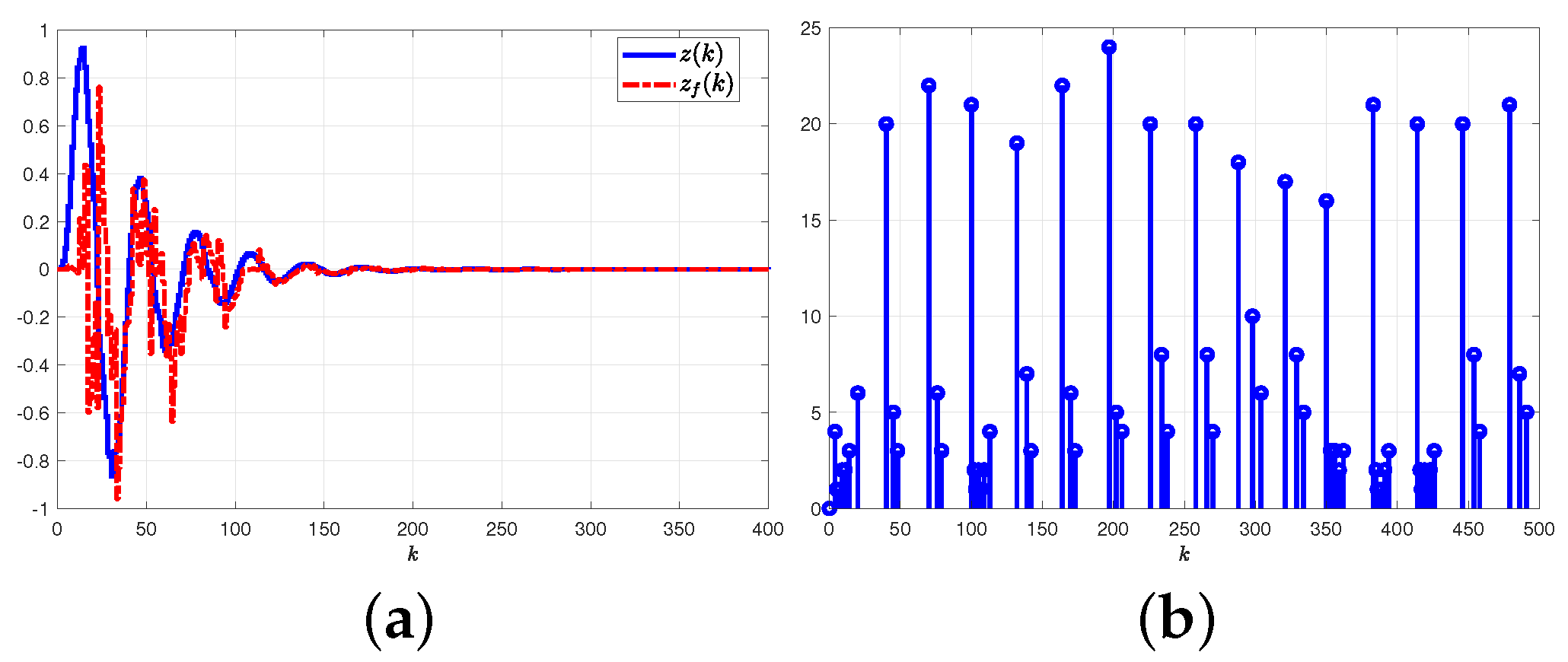
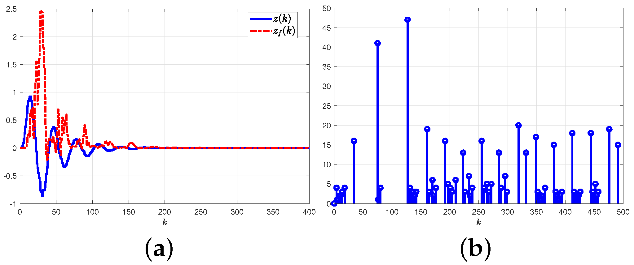
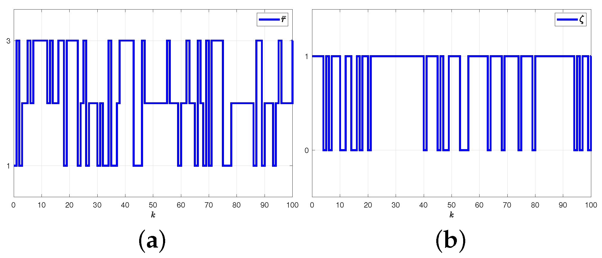
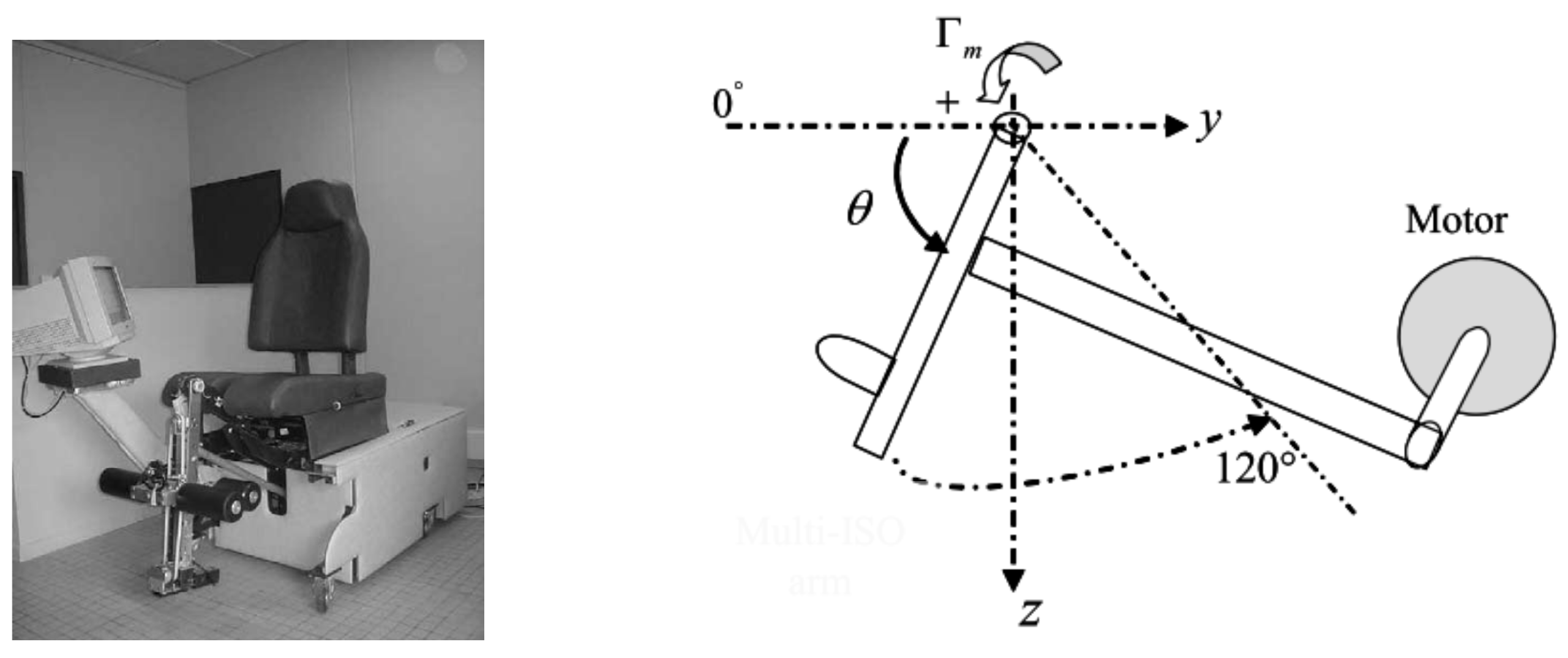
5.2. Single-Link Robot Arm System

Consider the single-link robot arm system described in [34] and stated as

$$\begin{array}{c}\hfill \left\{\begin{array}{cc}{x}_1(k+1)\hfill & =x_2\left(k\right)\hfill \\ x_2(k+1)\hfill & =-{\displaystyle \frac{m\left(\overline{r}\left(k\right)\right)gl{T}_e}{J\left(\overline{r}\left(k\right)\right)}}sin\left(x_1\left(k\right)\right)+(1-{\displaystyle \frac{D\left(\overline{r}\left(t\right)\right)T_e}{J\left(\overline{r}\left(t\right)\right)}})x_2\left(k\right)+{\displaystyle \frac{T_e}{J\left(\overline{r}\left(t\right)\right)}}u\left(k\right)\hfill \end{array}\right.\end{array}$$

(63)

with $x_1\left(k\right)$, $x_2\left(k\right)$, $m\left(\overline{r}\left(k\right)\right)$, $J\left(\overline{r}\left(k\right)\right)$, $D\left(\overline{r}\left(k\right)\right)$, and l being, respectively, the angle position, angle velocity, masses, moment of inertia, damping, and length of the robot arm, respectively. As in [34], the system can be converted into a Markov switching fuzzy system in the form of (4) with $T_s=0.1s$, and the related transition-probability matrix is defined as:

$$\mathsf{\Pi }=\left[\begin{array}{ccc}0.5& 0.25& 0.25\\ 2/14& 9/14& 3/14\\ 0.35& 0.15& 0.5\end{array}\right].$$

The considered model is described by the following system matrices:

$$\begin{array}{c}\hfill \begin{array}{cc}& {\mathit{A}}_1^1=\left[\begin{array}{cc}1& 0.1\\ -0.49& 0.7\end{array}\right],{\mathit{A}}_1^2=\left[\begin{array}{cc}1& 0.1\\ -0.43& 0.66\end{array}\right],{\mathit{A}}_1^3=\left[\begin{array}{cc}1& 0.1\\ -0.55& 0.68\end{array}\right],\hfill \\ & {\mathit{A}}_2^1=\left[\begin{array}{cc}1& 0.1\\ -0.42& 0.7\end{array}\right],A_2^2=\left[\begin{array}{cc}1& 0.1\\ -0.25v0.66\end{array}\right],{\mathit{A}}_2^3=\left[\begin{array}{cc}1& 0.1\\ -0.29& 0.68\end{array}\right]\hfill \\ & {\mathit{B}}_{wi}^p=\left[\begin{array}{c}0\\ 0.1\end{array}\right],{\mathit{C}}_{2i}^p=\left[\begin{array}{cc}1& 0\end{array}\right],{\mathit{C}}_{1i}^p=\left[\begin{array}{cc}0& 1\end{array}\right],{\mathit{D}}_{1i}^p=0,p=1,2,3.\hfill \end{array}\end{array}$$

(64)

The membership functions are defined as follows:

$$\begin{array}{cc}\hfill h_1\left(x_1\left(k\right)\right)& =\left\{\begin{array}{cc}{\displaystyle \frac{sin\left(x_1\left(k\right)\right)-{\beta }_0{x}_1\left(k\right)}{(1-{\beta }_0)x_1\left(k\right)}},\hfill & x_1\left(k\right)\ne 0\hfill \\ 1\hfill & x_1\left(k\right)=0\hfill \end{array}\right.\hfill \\ \hfill h_2\left(x_1\left(k\right)\right)& =\left\{\begin{array}{cc}{\displaystyle \frac{x_1\left(k\right)-sin\left(x_1\left(k\right)\right)}{(1-{\beta }_0)x_1\left(k\right)}},\hfill & x_1\left(k\right)\ne 0\hfill \\ 0\hfill & x_1\left(k\right)=0\hfill \end{array}\right.\hfill \end{array}$$

with ${\beta }_0={10}^{-2}/\pi$.

Next, we give the MFs of the filter. Define a nonlinear function as $l\left({\widehat{x}}_1\left(k\right)\right)={\widehat{x}}_1^2\left(k\right)$. For ${\widehat{x}}_1\left(k\right)\in [\pi -0.01,\pi +0.01]$, we have $l\left({\widehat{x}}_1\left(k\right)\right)\in [l_{min}\left({\widehat{x}}_1\left(k\right)\right),l_{max}\left({\widehat{x}}_1\left(k\right)\right)]$ with $l_{min}\left({\widehat{x}}_1\left(k\right)\right)=0$ and $l_{max}\left({\widehat{x}}_1\left(k\right)\right)={(\pi -0.01)}^2$. The MFs of the filter are given as ${\nu }_1(\widehat{x_1}\left(k\right))={\displaystyle \frac{l\left({\widehat{x}}_1\left(k\right)\right)-{\breve{l}}_{min}\left({\widehat{x}}_1\left(k\right)\right)}{{\breve{l}}_{max}\left({\widehat{x}}_1\left(k\right)\right)-{\breve{l}}_{min}\left({\widehat{x}}_1\left(k\right)\right)}}$ and ${\nu }_2(\widehat{x_1}\left(k\right))={\displaystyle \frac{{\breve{l}}_{max}\left({\widehat{x}}_1\left(k\right)\right)-l\left({\widehat{x}}_1\left(k\right)\right)}{{\breve{l}}_{max}\left({\widehat{x}}_1\left(k\right)\right)-{\breve{l}}_{min}\left({\widehat{x}}_1\left(k\right)\right)}}$ with ${\breve{l}}_{min}\left({\widehat{x}}_1\left(k\right)\right)=l_{min}\left({\widehat{x}}_1\left(k\right)\right)-0.1$ and ${\breve{l}}_{max}\left({\widehat{x}}_1\left(k\right)\right)={\pi }^2+0.1$.

For ${\tau }_m=1$, ${\tau }_M=5$, $\mathsf{\Theta }=3$, $\overline{\zeta }=0.8$, ${\varrho }_1=0.15$, ${\varrho }_2=1/0.15$, $\mathit{a}\left(k\right)=tanh\left(0.6y\right(k\left)\right)$, and $\mathit{G}=0.6$, Algorithm 1 is performed to design filters satisfying the extended dissipative performance from four aspects, namely $H_{\infty }$, $l_2-l_{\infty }$, passive, and dissipative performances. For the given cases,

Table 2. Minimal values for different performances.

Performance	${\mathsf{\Omega }}_1$	${\mathsf{\Omega }}_2$	${\mathsf{\Omega }}_3$	${\mathsf{\Omega }}_4$	${\mathit{a}}_1^{*}$	${\mathit{a}}_2^{*}$	${\mathit{b}}_1^{*}$	${\mathit{b}}_2^{*}$	${\mathit{\gamma }}^{*}$
$H_{\infty }$	−1	0	${\gamma }^2$	0	14.3165	−8.4295	14.5129	−9.4800	0.7327
passivity	0	1	$\gamma$	0	10.0000	−8.0000	14.5663	−10.0000	0.1201
dissipativity	−1	1	$\gamma$	0	10.6384	−8.0000	12.7780	−10.0000	$0.1238$

lists the minimum allowable values for $a_s$, $b_s,(s=1,2)$, and $\gamma$.

Then, we were concerned with different cases to conclude our discussion:

Case I: passivity filtering: 

$$\begin{array}{c}\hfill \begin{array}{cc}\hfill \left[\begin{array}{cccc}{\widehat{\mathit{A}}}_1^1& {\widehat{\mathit{A}}}_2^1& {\widehat{\mathit{B}}}_1^1& {\widehat{\mathit{B}}}_2^1\\ {\widehat{\mathit{A}}}_1^2& {\widehat{\mathit{A}}}_2^2& {\widehat{\mathit{B}}}_1^2& {\widehat{\mathit{B}}}_2^2\\ {\widehat{\mathit{A}}}_1^3& {\widehat{\mathit{A}}}_2^3& {\widehat{\mathit{B}}}_1^3& {\widehat{\mathit{B}}}_2^3\end{array}\right]& =\left[\begin{array}{cccccc}0.76238& 0.1182& 0.77373& 0.12784& 0.24699& 0.25917\\ -0.85348& 0.31808& -0.70568& 0.31865& 0.076161& 0.20964\\ ine0.62687& 0.078345& 0.68218& 0.059552& 0.33982& 0.42384\\ -1.4991& 0.26763& -1.3146& 0.20334& 0.40852& 1.2533\\ ine0.68872& 0.085852& 0.70391& 0.10369& 0.28929& 0.39769\\ -1.2972& 0.2118& -0.92588& 0.17481& 0.078596& 0.83558\end{array}\right]\hfill \\ \hfill \left[\begin{array}{cc}{\widehat{\mathit{C}}}_1^1& {\widehat{\mathit{C}}}_2^1\\ {\widehat{\mathit{C}}}_1^2& {\widehat{\mathit{C}}}_2^2\\ {\widehat{\mathit{C}}}_1^3& {\widehat{\mathit{C}}}_2^3\end{array}\right]& =\left[\begin{array}{cccc}-0.38676& 0.10875& -0.38987& 0.10831\\ ine-0.57935& 0.11218& -0.58156& 0.11422\\ ine-0.47562& 0.087605& -0.49095& 0.084071\end{array}\right]\hfill \end{array}\end{array}$$

(65)

Case II: dissipativity filtering: 

$$\begin{array}{c}\hfill \begin{array}{cc}\hfill \left[\begin{array}{cccc}{\widehat{\mathit{A}}}_1^1& {\widehat{\mathit{A}}}_2^1& {\widehat{\mathit{B}}}_1^1& {\widehat{\mathit{B}}}_2^1\\ {\widehat{\mathit{A}}}_1^2& {\widehat{\mathit{A}}}_2^2& {\widehat{\mathit{B}}}_1^2& {\widehat{\mathit{B}}}_2^2\\ {\widehat{\mathit{A}}}_1^3& {\widehat{\mathit{A}}}_2^3& {\widehat{\mathit{B}}}_1^3& {\widehat{\mathit{B}}}_2^3\end{array}\right]& =\left[\begin{array}{cccccc}0.75035& 0.10162& 0.76625& 0.115& 0.26128& 0.27117\\ -0.67407& 0.53154& -0.51703& 0.53359& 0.076572& 0.19088\\ ine0.56972& 0.052941& 0.63612& 0.027462& 0.34737& 0.47697\\ -1.3854& 0.46117& -1.216& 0.38875& 0.45019& 1.3471\\ ine0.60712& 0.041119& 0.61428& 0.053424& 0.30315& 0.52321\\ -1.4628& 0.3626& -1.1198& 0.28418& 0.19734& 1.4148\end{array}\right]\hfill \\ \hfill \left[\begin{array}{cc}{\widehat{\mathit{C}}}_1^1& {\widehat{\mathit{C}}}_2^1\\ {\widehat{\mathit{C}}}_1^2& {\widehat{\mathit{C}}}_2^2\\ {\widehat{\mathit{C}}}_1^3& {\widehat{\mathit{C}}}_2^3\end{array}\right]& =\left[\begin{array}{cccc}-0.32311& 0.15403& -0.32593& 0.15345\\ ine-0.61589& 0.16114& -0.61878& 0.16324\\ ine-0.4861& 0.088156& -0.50649& 0.085026\end{array}\right]\hfill \end{array}\end{array}$$

(66)

Case III: $H_{\infty }$ filtering:

$$\begin{array}{c}\hfill \begin{array}{cc}\hfill \left[\begin{array}{cccc}{\widehat{\mathit{A}}}_1^1& {\widehat{\mathit{A}}}_2^1& {\widehat{\mathit{B}}}_1^1& {\widehat{\mathit{B}}}_2^1\\ {\widehat{\mathit{A}}}_1^2& {\widehat{\mathit{A}}}_2^2& {\widehat{\mathit{B}}}_1^2& {\widehat{\mathit{B}}}_2^2\\ {\widehat{\mathit{A}}}_1^3& {\widehat{\mathit{A}}}_2^3& {\widehat{\mathit{B}}}_1^3& {\widehat{\mathit{B}}}_2^3\end{array}\right]& =\left[\begin{array}{cccccc}0.8641& 0.074582& 0.88691& 0.092459& 0.15007& 0.15425\\ -0.44428& 0.7861& -0.30547& 0.78572& -0.038087& -0.02165\\ ine0.64921& -0.017533& 0.83116& 0.06009& 0.2362& 0.31973\\ -0.45812& 0.74357& -0.091925& 0.70545& 0.017246& 0.1741\\ ine0.33701& -0.15945& 0.24163& -0.10596& 0.1781& 1.7443\\ -1.0908& 0.47433& -1.3547& 0.57936& -0.42549& 2.786\end{array}\right]\hfill \\ \hfill \left[\begin{array}{cc}{\widehat{\mathit{C}}}_1^1& {\widehat{\mathit{C}}}_2^1\\ {\widehat{\mathit{C}}}_1^2& {\widehat{\mathit{C}}}_2^2\\ {\widehat{\mathit{C}}}_1^3& {\widehat{\mathit{C}}}_2^3\end{array}\right]& =\left[\begin{array}{cccc}0.00036846& 0.63323& 0.014015& 0.63422\\ ine-0.070462& 0.57629& 5.1593.{10}^{-6}& 0.47536\\ ine-0.16548& 0.51958& 0.042926& 0.52235\end{array}\right]\hfill \end{array}\end{array}$$

(67)

Case IV: $H_{\infty }$ 

filtering in [34]: In this case, we used the filter proposed in [34] with a constant threshold $\sigma =0.5$.

For the first three cases, the gains were calculated by employing the minimal values recorded in Table 2.

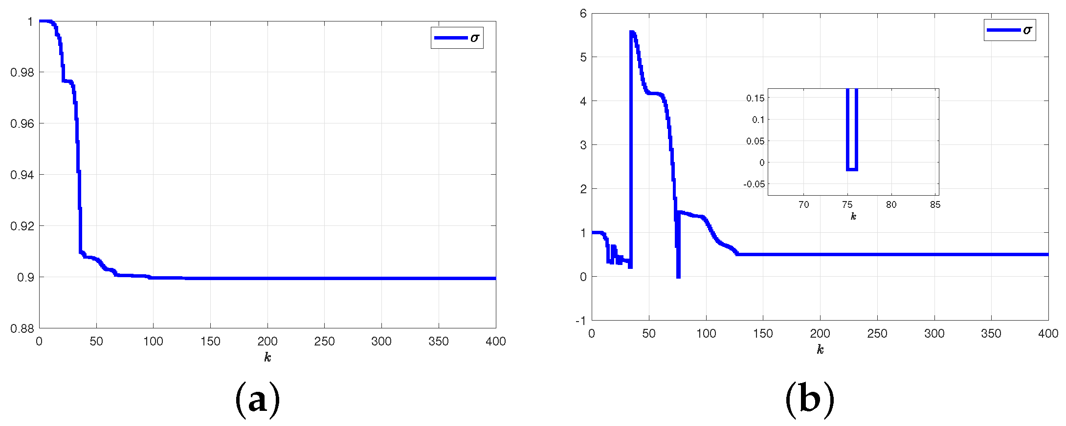
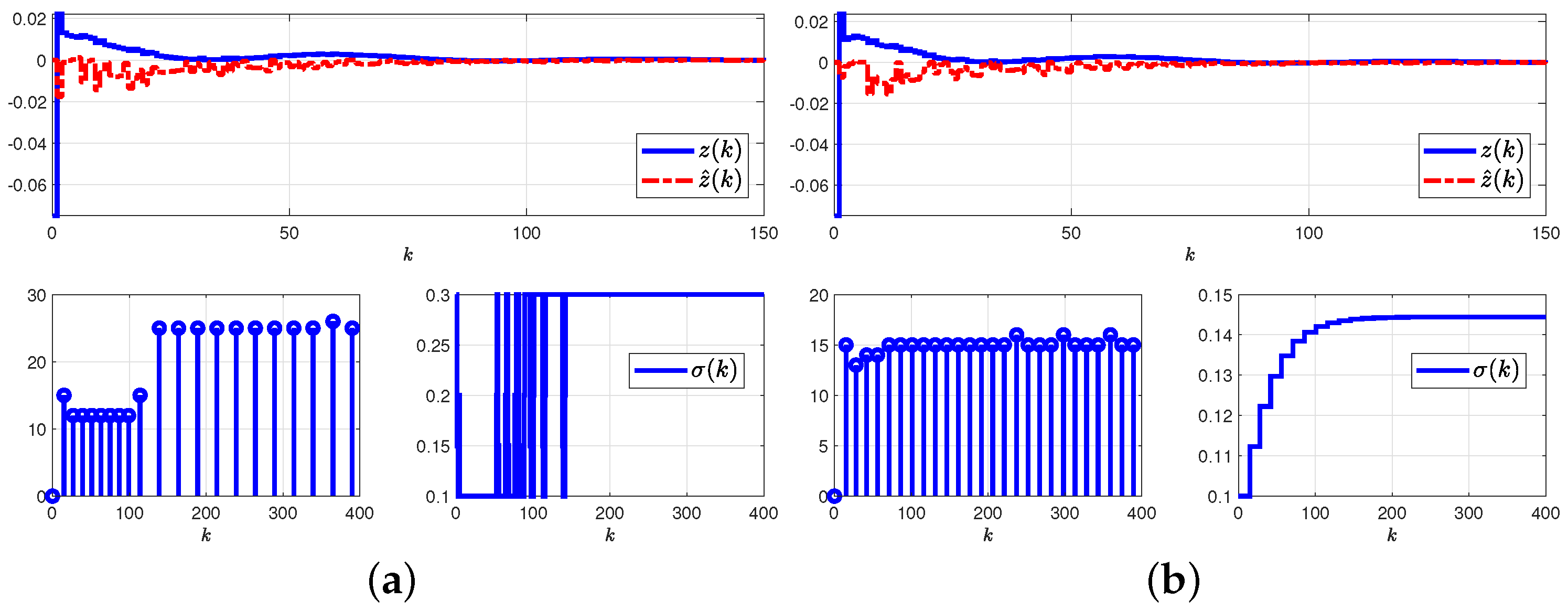
5.2.1. Results and Graphical Plots

Given the initial conditions $x\left(0\right)=\widehat{x}\left(0\right)={\left[\begin{array}{cc}0& 0\end{array}\right]}^T$, the numerical simulations were performed for $w\left(k\right)=8si{n}^2\left(k\right)e^{-0.3k}$. For different cases, the simulation results are depicted in Figure 2, Figure 3, Figure 4 and Figure 5, where the switching signal $\overline{r}\left(k\right)$ and Bernoulli distribution are, respectively, depicted in Figure 6a,b.

5.2.2. Comparative Explanations

Figure 2a, Figure 3a, Figure 4a, Figure 5a display the output $\mathit{z}\left(k\right)$ and its estimation $\widehat{\mathit{z}}\left(k\right)$. Figure 2b, Figure 3b, Figure 4, Figure 5b show the event-triggered release instants and the intervals. According to the time-triggered schemes, the percentages of transmitted data for different cases are shown in

Table 3. Data transmission rate, ISE, and IAE for different cases.

Filter Gains	(65)	(66)	(67)	[34]
Data transmission rate	14.172	13.573	12.575	18.563
ISE	1.5152	1.4895	0.94308	8.7833
IAE	2.9001	2.8546	2.4904	5.8065

. Moreover, the table provides an overview of the comparison using a quantitative analysis, where the deviations of the state error $\widehat{\mathit{e}}\left(k\right)$ are investigated by computing the integral squared error (ISE) and the integral absolute error (IAE) for different filters. In light of our results, we can substantiate that our method effectively mitigates the waste of computational resources and communication channels, with the smallest total deviation of $\widehat{\mathit{e}}\left(k\right)$. To evaluate the merit of the proposed approach, the adaptive ET scheme proposed by [48] was applied to the system, as shown in Figure 7b. Using the AET mechanism described in [48], the adaptive variable showed clearly a negative value, which is inaccurate.

5.3. A Lower Limbs Rehabilitation System

As shown in Figure 8, this example uses an isokinetic rehabilitation system for the lower limbs, which can assist the handicapped in Hail is described by the following differential nonlinear equation [61]:

$$\begin{array}{c}\hfill {\Gamma }_m=J_m\ddot{\theta }+f_m\theta -k_m{\displaystyle \frac{\dot{\theta }}{|\dot{\theta }|}}{\dot{\theta }}^2-Fl-acos\left(\theta \right)-bsin\left(\theta \right)\end{array}$$

(68)

${\Gamma }_m$, $J_m$, and $f_m$, respectively, represent the controlled variables that determine the torque, inertia, and viscous friction. Moreover, the variables $\ddot{\theta }$, $\dot{\theta }$, and $\theta$ correspond to the angular position, velocity, and acceleration of the mobile part. The torque delivered by the patient is described by F times l; the potential energy of the system is described by $acos\left(\theta \right)$; the centrifugal force coefficient is described by $bsin\left(\theta \right)$, while the centrifugal force coefficient needs to be added or subtracted according to the velocity sign. Define $\mathit{x}\left(t\right)=[x_1\left(t\right),x_2\left(t\right)]=[\dot{\theta },\theta ]$, $u\left(t\right)={\Gamma }_m$, and $w\left(t\right)=F$. A discrete-time model of System (68) can be obtained by applying Euler’s discretization:

$$\begin{array}{c}\hfill \left\{\begin{array}{cc}{x}_1(k+1)\hfill & =(1+T_{s}g(k_m,x_1\left(k\right)))x_1\left(k\right)+T_{s}f\left(x_2\left(k\right)\right)x_2\left(k\right)+{\displaystyle \frac{T_s}{J_m}}u\left(k\right)+{\displaystyle \frac{T_{s}l}{J_m}}w\left(k\right)\hfill \\ x_2(k+1)\hfill & =x_2\left(k\right)+T_s\left(k\right)\hfill \end{array}\right.\end{array}$$

(69)

with $g(k_m,x_1\left(k\right))={\displaystyle \frac{k_m\left|x_1\left(k\right)\right|-f_m}{J_m}}$ and $f\left(x_2\left(k\right)\right)={\displaystyle \frac{acos\left(x_2\left(k\right)\right)-bsin\left(x_2\left(k\right)\right)}{J_m{x}_2\left(k\right)}}$.

A list of the parameters of the system can be found in

Table 4. Markov mode parameters of the system.

Parameter	Physical Meaning	Value	Mode 1	Mode 2	Unit
a	Gravitational coefficient	110	-	-	(N)
b	Gravitational coefficient	31	-	-	(N)
l	Arm’s length	$0.5$	-	-	(m)
$f_m$	Viscous friction	$103.6$	-	-	(N(rad/s)${}^{-1}$)
$k_m$	Coriolis coefficient	$[70,80]$	-	-	(Nm(rad/s)${}^{-1}$)
$J_m$	inertia	-	33.8	35.2	(kg m${}^{-2}$)

. As a further consideration, it was assumed that parameter $J_m$ has two different modes, listed in the table. Given the uncertainty associated with the parameter $k_m$, it is evident that the IT-2 fuzzy system should be adopted to model a nonlinear system (68). Assume that $x_1\left(k\right)\in [-2\pi ,2\pi ]$ and $x_2\left(k\right)\in [\pi /180,2\pi /3]$; we can obtain $g_{max}=-3.0651$ and $g_{min}=11.806$, and $g\left(x_1\left(k\right)\right)\in [{\overline{g}}_{max},{\overline{g}}_{min}]=[-4,12]$.

By adopting the sector nonlinearity method, the membership functions of the corresponding IT-2 fuzzy model are defined as

$$\begin{array}{cccc}\hfill {\mu }_1\left(x_1\left(k\right)\right)& =m_1\left(x_1\left(k\right)\right)h_1\left(x_2\left(k\right)\right),\hfill & \hfill {\mu }_2\left(x_1\left(k\right)\right)& =m_2\left(x_1\left(k\right)\right)h_2\left(x_2\left(k\right)\right),\hfill \\ \hfill {\mu }_3\left(x_1\left(k\right)\right)& =m_1\left(x_1\left(k\right)\right)h_1\left(x_2\left(k\right)\right),\hfill & \hfill {\mu }_4\left(x_1\left(k\right)\right)& =m_2\left(x_1\left(k\right)\right)h_2\left(x_2\left(k\right)\right)\hfill \end{array}$$

with $m_i\left(x_1\left(k\right)\right)={\underline{m}}_i\left(x_1\left(k\right)\right){sin}^2\left(x_1\left(k\right)\right)+{\overline{m}}_i\left(x_1\left(k\right)\right){cos}^2\left(x_1\left(k\right)\right)$, ${\underline{m}}_1\left(x_1\left(k\right)\right)=$${\displaystyle \frac{{\overline{g}}_{max}-g(80,x_1\left(k\right))}{{\overline{g}}_{max}-{\overline{g}}_{min}}}$, ${\overline{m}}_1\left(x_1\left(k\right)\right)={\displaystyle \frac{g_{max}-g(70,x_1\left(k\right))}{{\overline{g}}_{max}-{\overline{g}}_{min}}}$, ${\underline{m}}_2\left(x_1\left(k\right)\right)=1-{\overline{m}}_1\left(x_1\left(k\right)\right)$, ${\overline{m}}_2\left(x_1\left(k\right)\right)=1-{\underline{m}}_1\left(x_1\left(k\right)\right)$, $h_1\left(x_2\left(k\right)\right)={\displaystyle \frac{187.35-f\left(x_2\left(k\right)\right)}{187.75}}$, and $h_2\left(x_2\left(k\right)\right)=1-h_1\left(x_2\left(k\right)\right)$.

Thus, the dynamical model of (68) can be described by the Markov switching fuzzy system in the form of (4) with $T_s=0.025$ s, and the transition probability rate matrix and the system matrices are defined as:

$$\begin{array}{c}\hfill \begin{array}{cc}& A_1^1=\left[\begin{array}{cc}-0.2557& -6.1348\\ 0.0250& 1.0000\end{array}\right],A_2^1=\left[\begin{array}{cc}-0.2561& -1.3733\\ 0.0250& 1.0000\end{array}\right],A_3^1=\left[\begin{array}{cc}0.0706& -6.0071\\ 0.0250& 1.0000\end{array}\right],\hfill \\ & A_4^1=\left[\begin{array}{cc}0.0706& -1.4156\\ 0.0250& 1.0000\end{array}\right],A_1^2=\left[\begin{array}{cc}-0.2488& -6.0116\\ 0.0250& 1.0000\end{array}\right],A_2^2=\left[\begin{array}{cc}-0.2487& -1.4191\\ 0.0250& 1.00001\end{array}\right],\hfill \\ & A_3^2=\left[\begin{array}{cc}0.0649& -5.8815\\ 0.0250& 1.0000\end{array}\right],A_4^2=\left[\begin{array}{cc}0.0644& -1.4777\\ 0.0250& 1.0000\end{array}\right],B_i^1=\left[\begin{array}{c}0.00037\\ 0\end{array}\right],B_i^2=\left[\begin{array}{c}0.000355\\ 0\end{array}\right],\hfill \\ & \mathsf{\Pi }=\left[\begin{array}{cc}0.7& 0.3\\ 0.2& 0.8\end{array}\right]\hfill \end{array}\end{array}$$

(70)

For ${\tau }_m=2$, ${\tau }_M=6$, $\mathsf{\Theta }=5$, $\overline{\zeta }=0.85$, ${\varrho }_1=0.15$, and ${\varrho }_2=1/0.15$, Algorithm 1 was performed, and the optimal values of the $l_2-l_{\infty }$ performance were obtained as: $a_1^{*}=2.0581$, $a_2^{*}=2.5176$, $b_1^{*}-0.1309$$b_2^{*}=-0.1744$, and ${\gamma }^{*}=7.{223}^{-4}$. The filter matrices are designed as

$$\begin{array}{c}\hfill \begin{array}{cc}\hfill & \left[\begin{array}{cccc}{\widehat{\mathit{A}}}_1^1& {\widehat{\mathit{A}}}_2^1& {\widehat{\mathit{A}}}_3^1& {\widehat{\mathit{A}}}_4^1\\ {\widehat{\mathit{A}}}_1^2& {\widehat{\mathit{A}}}_2^2& {\widehat{\mathit{A}}}_3^2& {\widehat{\mathit{A}}}_4^2\end{array}\right]=\hfill \\ \hfill & \left[\begin{array}{cccccccc}0.073469& -3.4221& 0.083413& -0.6332& 0.20643& -3.2698& 0.21936& -0.73011\\ 0.01021& 0.926& 0.0076208& 0.97167& 0.011397& 0.92152& 0.012629& 0.97586\\ ine-0.060213& -2.8422& -0.092627& -0.75619& 0.17697& -2.6329& 0.19582& -0.79572\\ 0.013459& 0.93971& 0.010413& 0.96712& 0.014624& 0.93769& 0.018435& 0.97071\end{array}\right]\hfill \\ \hfill & \left[\begin{array}{cccc}{\widehat{\mathit{B}}}_1^1& {\widehat{\mathit{B}}}_2^1& {\widehat{\mathit{B}}}_3^1& {\widehat{\mathit{B}}}_4^1\\ {\widehat{\mathit{B}}}_1^2& {\widehat{\mathit{B}}}_2^2& {\widehat{\mathit{B}}}_3^2& {\widehat{\mathit{B}}}_4^2\end{array}\right]=\hfill \\ \hfill & \left[\begin{array}{cccc}-9.5398& 9.3138& -8.6087& 6.7673\\ -0.0038308& 0.32511& -0.042507& 0.38779\\ ine-7.5654& 6.6368& -6.6323& 5.2521\\ 0.041711& 0.28217& 0.019727& 0.29285\end{array}\right]\hfill \\ \hfill & \left[\begin{array}{cccc}{\widehat{\mathit{C}}}_1^1& {\widehat{\mathit{C}}}_2^1& {\widehat{\mathit{C}}}_3^1& {\widehat{\mathit{C}}}_4^1\\ {\widehat{\mathit{C}}}_1^2& {\widehat{\mathit{C}}}_2^2& {\widehat{\mathit{C}}}_3^2& {\widehat{\mathit{C}}}_4^2\end{array}\right]=\hfill \\ \hfill & \left[\begin{array}{cccccccc}0.029365& 0.015436& 0.029365& 0.015436& 0.029365& 0.015436& 0.029365& 0.015436\\ ine0.044923& 0.026018& 0.044923& 0.026018& 0.044923& 0.026018& 0.044923& 0.026018\end{array}\right]\hfill \end{array}\end{array}$$

(71)

According to the above parameters, the simulation results are presented in Figure 9, Figure 10 and Figure 11, where Figure 11b illustrates, respectively, the random variables $\overline{r}\left(k\right)$ and $\zeta \left(k\right)$. As an intuitive method for evaluating the communication performance of the designed filter, Figure 9a, Figure 10a, Figure 11a record the trajectories of the system’s and filter’s outputs, the triggering instants and intervals of each system state component, as well as the dynamic threshold parameters for the different trigger mechanisms suggested in [35,48,53,54]. As can be seen in these figures, the implemented filter for different ETMs can guarantee the convergence of the system’s states despite uncertainties, external disturbances, and cyber-attacks. Based on

Table 5. Number and rate of transmitted data packets and IAE for different event-triggered mechanisms.

Event-Triggered Mechanism	Packets Transmitted	Data Transmission Rate (%)	IAE (%)
Proposed	12	2.99	1.69
[35]	20	4.98	1.74
[48]	14	3.49	1.67
[53]	19	4.74	1.81
[54]	26	6.48	1.67

, it appears that the application of the AETM in this article may further optimize communication resources and reduce bandwidth usage because the number of data packets transmitted with an acceptable IAE was significantly less than the number of data packets transmitted using the ETMs in [35,48,53,54,62].

5.4. Comparative Explanations

The dynamic- and adaptive-event-triggered filtering problem for nonlinear networks has recently been the subject of numerous studies in the literature, so several methods are comparable to what we presented here. There are, however, some differences from our approaches as follows:

• To handle nonlinear network systems, a $H_{\infty }$ linear filter was designed in [26] using Type-1 fuzzy models, which may lead to conservative results. As an alternative, we took a more general approach based on a Markovian jump Type-2 fuzzy model to design an IT2 fuzzy filter with extended dissipativity performance.
• Different from [49,62], the filter design method described in [26] was based on an improved matrix decoupling approach that uses appropriate selected scalars. The selection of these parameters can be achieved either by a numerical analysis or by using meta-heuristic techniques, such as the PSO method addressed in this study.

6. Conclusions, Limitations, and Future Work

Some conclusions, possibilities for future developments, and limitations of the filtering strategy are presented in this section.

6.1. Concluding Remarks

For a class of nonlinear discrete-time systems described by Markov jumping IT-2 fuzzy models, a novel adaptive-event-triggered extended dissipativity-based filtering problem was developed. This study successfully addressed the hypothesis of perturbations and the random occurrence of cyber-attacks. As a means of reducing the unnecessary use of limited communication resources, a new event-triggered scheme with an adaptive triggering scheme was used to determine whether or not the current measurements needed to be transmitted. Furthermore, delay-dependent conditions were developed for the filter design in order to ensure that the error system would be stochastically stable with extended dissipativity performance. Using the upper and lower membership functions, less conservative results were obtained. Furthermore, an optimization-based algorithm (PSO) was used for the determination of the filter gains and to achieve the best-possible performance. Finally, this paper concluded with two examples that illustrated how effective the method proposed here can be.

6.2. Limitations

Despite the power and performance of the synthesized technique, the latter imposes that the Markov chain transition probability is known as a delicate task in practice. Equally important, the synchronization between modes of the filter and model is a task that may be difficult to achieve in practice.

6.3. Future Work

Further research that may be focused on in the context of the present study is related to the state estimation of singular systems based on the dynamic-event-triggered communication protocol [56,63]. Moreover, the determination of partial and time-varying transition probabilities in our framework is an open problem to be addressed in the future.

References

1. Hou, L.; Chen, D.; He, C. Finite-time nonfragile dissipative control for discrete-time neural networks with Markovian jumps and mixed time-delays. Complexity 2019, 2019, 5748923. [Google Scholar] [CrossRef]
2. Sathishkumar, M.; Sakthivel, R.; Alzahrani, F.; Kaviarasan, B.; Ren, Y. Mixed H and passivity-based resilient controller for nonhomogeneous Markovian jump systems. Nonlinear Anal. Hybrid Syst. 2019, 31, 86–99. [Google Scholar] [CrossRef]
3. Cheng, J.; Park, J.H.; Cao, J.; Qi, W. A hidden mode observation approach to finite-time SOFC of Markovian switching systems with quantization. Nonlinear Dyn. 2020, 100, 509–521. [Google Scholar] [CrossRef]
4. Cheng, J.; Park, J.H.; Zhao, X.; Karimi, H.R.; Cao, J. Quantized Nonstationary Filtering of Networked Markov Switching RSNSs: A Multiple Hierarchical Structure Strategy. IEEE Trans. Autom. Control. 2020, 65, 4816–4823. [Google Scholar] [CrossRef]
5. Li, H.; Shi, P.; Yao, D.; Wu, L. Observer-based adaptive sliding mode control for nonlinear Markovian jump systems. Automatica 2016, 64, 133–142. [Google Scholar] [CrossRef]
6. Ma, Y.; Jia, X.; Zhang, Q. Robust finite-time non-fragile memory H control for discrete-time singular Markovian jumping systems subject to actuator saturation. J. Frankl. Inst. 2017, 354, 8256–8282. [Google Scholar] [CrossRef]
7. Wu, B.; Zhao, Y. Dissipative Control for Fuzzy Singular Markov Jump Systems With State-Dependent Noise and Asynchronous Modes. IEEE Access 2021, 9, 25691–25702. [Google Scholar] [CrossRef]
8. Qi, W.; Park, J.; Cheng, J.; Chen, X. Stochastic stability and L1-gain analysis for positive nonlinear semi-Markovian jump systems with time-varying delay via TS fuzzy model approach. Fuzzy Sets Syst. 2019, 371, 110–122. [Google Scholar] [CrossRef]
9. Kavikumar, R.; Sakthivel, R.; Kwon, O.; Kaviarasan, B. Reliable non-fragile memory state feedback controller design for fuzzy Markovian jump systems. Nonlinear Anal. Hybrid Syst. 2020, 35, 100828. [Google Scholar] [CrossRef]
10. Tian, Y.; Wang, Z. Asynchronous Extended Dissipative Filtering for T-S Fuzzy Markov Jump Systems. IEEE Trans. Syst. Man Cybern. Syst. 2022, 52, 3915–3925. [Google Scholar] [CrossRef]
11. Li, J.; Zhang, Q.; Yan, X.G.; Spurgeon, S.K. Integral sliding mode control for Markovian jump T-S fuzzy descriptor systems based on the super-twisting algorithm. Iet Control. Theory Appl. 2017, 11, 1134–1143. [Google Scholar] [CrossRef]
12. Lv, C.; Chen, J.; Lv, X.; Zhang, Z. Finite-time H control for interval Type-2 fuzzy singular systems via switched fuzzy models and static output feedback. Nonlinear Anal. Hybrid Syst. 2022, 45, 101206. [Google Scholar] [CrossRef]
13. Zhao, T.; Wei, Z.; Dian, S.; Xiao, J. Observer-based H controller design for interval Type-2 T-S fuzzy systems. Neurocomputing 2016, 177, 9–25. [Google Scholar] [CrossRef]
14. Song, W.; Tong, S. Fuzzy decentralized output feedback event-triggered control for interval Type-2 fuzzy systems with saturated inputs. Inf. Sci. 2021, 575, 639–653. [Google Scholar] [CrossRef]
15. Alshammari, O.; Kchaou, M.; Jerbi, H.; Ben Aoun, S.; Leiva, V. A Fuzzy Design for a Sliding Mode Observer-Based Control Scheme of Takagi–Sugeno Markov Jump Systems under Imperfect Premise Matching with Bio-Economic and Industrial Applications. Mathematics 2022, 10, 3309. [Google Scholar] [CrossRef]
16. Wang, S.; Feng, J.; Zhang, H. Robust fault tolerant control for a class of networked control systems with state delay and stochastic actuator failures. Int. J. Adapt. Control. Signal Process. 2014, 28, 798–811. [Google Scholar] [CrossRef]
17. Latrech, C.; Kchaou, M.; Guéguen, H. Networked non-fragile H static output feedback control design for vehicle dynamics stability: A descriptor approach. Eur. J. Control. 2018, 40, 13–26. [Google Scholar] [CrossRef]
18. Wang, B.; Chen, W.; Wang, J.; Zhang, B.; Zhang, Z.; Qiu, X. Cooperative Tracking Control of Multiagent Systems: A Heterogeneous Coupling Network and Intermittent Communication Framework. IEEE Trans. Cybern. 2019, 49, 4308–4320. [Google Scholar] [CrossRef]
19. Li, Q.; Wang, Z.; Sheng, W.; Alsaadi, F.E.; Alsaadi, F.E. Dynamic event-triggered mechanism for H non-fragile state estimation of complex networks under randomly occurring sensor saturations. Inf. Sci. 2020, 509, 304–316. [Google Scholar] [CrossRef]
20. Chen, M.; Karimi, H.R.; Sun, J. Observer-based finite time H control of nonlinear discrete time-varying systems with an adaptive-event-triggered Mechanism. J. Frankl. Inst. 2020, 357, 11668–11689. [Google Scholar] [CrossRef]
21. Chu, X.; Li, M. H non-fragile observer-based dynamic-event-triggered sliding mode control for nonlinear networked systems with sensor saturation and dead-zone input. ISA Trans. 2019, 94, 93–107. [Google Scholar] [CrossRef] [PubMed]
22. Qi, W.; Zong, G.; Zheng, W.X. Adaptive Event-Triggered SMC for Stochastic Switching Systems With Semi-Markov Process and Application to Boost Converter Circuit Model. IEEE Trans. Circuits Syst. I: Regul. Pap. 2021, 68, 786–796. [Google Scholar] [CrossRef]
23. Zhang, Y.; Shi, P.; Agarwal, R.K.; Shi, Y. Event-Based Dissipative Analysis for Discrete Time-Delay Singular Jump Neural Networks. IEEE Trans. Neural Netw. Learn. Syst. 2020, 31, 1232–1241. [Google Scholar] [CrossRef]
24. Wang, X.L.; Yang, G.H. Event-triggered fault detection for discrete-time T-S fuzzy systems. ISA Trans. 2018, 76, 18–30. [Google Scholar] [CrossRef] [PubMed]
25. Song, X.; Men, Y.; Zhou, J.; Zhao, J.; Shen, H. Event-triggered H control for networked discrete-time Markov jump systems with repeated scalar nonlinearities. Appl. Math. Comput. 2017, 298, 123–132. [Google Scholar] [CrossRef]
26. Chen, Q.X.; Chang, X.H. Resilient filter of nonlinear network systems with dynamic event-triggered mechanism and hybrid cyber-attack. Appl. Math. Comput. 2022, 434, 127419. [Google Scholar] [CrossRef]
27. Tian, E.; Wang, Z.; Zou, L.; Yue, D. Probabilistic-constrained filtering for a class of nonlinear systems with improved static event-triggered communication. Int. J. Robust Nonlinear Control. 2019, 29, 1484–1498. [Google Scholar] [CrossRef]
28. Liu, J.; Zhang, N.; Li, Y.; Xie, X. H filter design for discrete-time networked systems with adaptive-event-triggered mechanism and hybrid cyber-attacks. J. Frankl. Inst. 2021, 358, 9325–9345. [Google Scholar] [CrossRef]
29. Dong, S.; Fang, M.; Shi, P.; Wu, Z.G.; Zhang, D. Dissipativity-Based Control for Fuzzy Systems With Asynchronous Modes and Intermittent Measurements. IEEE Trans. Cybern. 2020, 50, 2389–2399. [Google Scholar] [CrossRef]
30. Liu, J.; Yin, T.; Cao, J.; Yue, D.; Karimi, H.R. Security Control for T-S Fuzzy Systems With Adaptive Event-Triggered Mechanism and Multiple Cyber-Attacks. IEEE Trans. Syst. Man Cybern. Syst. 2021, 51, 6544–6554. [Google Scholar] [CrossRef]
31. Hsieh, C.S. Robust two-stage Kalman filters for systems with unknown inputs. IEEE Trans. Autom. Control. 2000, 45, 2374–2378. [Google Scholar] [CrossRef]
32. Jwo, D.J.; Wang, S.H. Adaptive Fuzzy Strong Tracking Extended Kalman Filtering for GPS Navigation. IEEE Sens. J. 2007, 7, 778–789. [Google Scholar] [CrossRef]
33. Hamid, K.R.; Talukder, A.; Islam, A.K.M.E. Implementation of Fuzzy Aided Kalman Filter for Tracking a Moving Object in Two-Dimensional Space. Int. J. Fuzzy Log. Intell. Syst. 2018, 18, 85–96. [Google Scholar] [CrossRef]
34. Zhang, M.; Shi, P.; Liu, Z.; Ma, L.; Su, H. H filtering for discrete-time switched fuzzy systems with randomly occurring time-varying delay and packet dropouts. Signal Process. 2018, 143, 320–327. [Google Scholar] [CrossRef]
35. Wang, H.; Xue, A. Adaptive event-triggered H filtering for discrete-time delayed neural networks with randomly occurring missing measurements. Signal Process. 2018, 153, 221–230. [Google Scholar] [CrossRef]
36. Zhang, J.; Peng, C. Event-triggered H filtering for networked Takagi–Sugeno fuzzy systems with asynchronous constraints. IET Signal Process. 2015, 9, 403–411. [Google Scholar] [CrossRef]
37. Zhang, Y.; Shi, P.; Agarwal, R.K.; Shi, Y. Event-based mixed H and passive filtering for discrete singular stochastic systems. Int. J. Control. 2020, 93, 2407–2415. [Google Scholar] [CrossRef]
38. Tian, Y.; Wang, Z. Finite-Time Extended Dissipative Filtering for Singular T-S Fuzzy Systems With Nonhomogeneous Markov Jumps. IEEE Trans. Cybern. 2022, 52, 4574–4584. [Google Scholar] [CrossRef]
39. Shi, P.; Su, X.; Li, F. Dissipativity-Based Filtering for Fuzzy Switched Systems with Stochastic Perturbation. IEEE Trans. Autom. Control. 2016, 61, 1694–1699. [Google Scholar] [CrossRef]
40. Cheng, J.; Park, J.H.; Chadli, M. Peak-to-peak fuzzy filtering of nonlinear discrete-time systems with Markov communication protocol. Inf. Sci. 2022, 607, 361–376. [Google Scholar] [CrossRef]
41. Song, J.; Chang, X.H. Finite-Time Peak-To-Peak Filtering for Nonlinear Singular System. IEEE Trans. Circuits Syst. Ii: Express Briefs 2022, 69, 4369–4373. [Google Scholar] [CrossRef]
42. Kchaou, M.; Regaieg, M.A.; Al-Hajjaji, A. Quantized asynchronous extended dissipative observer-based sliding mode control for Markovian jump TS fuzzy systems. J. Frankl. Inst. 2022, 359, 9636–9665. [Google Scholar] [CrossRef]
43. Liu, J.; Gu, Y.; Cao, J.; Fei, S. Distributed event-triggered H filtering over sensor networks with sensor saturations and cyber-attacks. ISA Trans. 2018, 81, 63–75. [Google Scholar] [CrossRef] [PubMed]
44. Zhang, J.; Christofides, P.D.; He, X.; Wu, Z.; Zhang, Z.; Zhou, D. Event-triggered filtering and intermittent fault detection for time-varying systems with stochastic parameter uncertainty and sensor saturation. Int. J. Robust Nonlinear Control. 2018, 28, 4666–4680. [Google Scholar] [CrossRef]
45. Wu, Y.; Cheng, J.; Wu, Z.G. Fuzzy-Affine-Model-Based Filtering Design With Memory-Based Dynamic Event-Triggered Protocol. IEEE Trans. Fuzzy Syst. 2022, 1–11. [Google Scholar] [CrossRef]
46. Peng, C.; Zhang, J.; Yan, H. Adaptive Event-Triggering H Load Frequency Control for Network-Based Power Systems. IEEE Trans. Ind. Electron. 2018, 65, 1685–1694. [Google Scholar] [CrossRef]
47. Gu, Z.; Yue, D.; Liu, J.; Ding, Z. H tracking control of nonlinear networked systems with a novel adaptive-event-triggered communication scheme. J. Frankl. Inst. 2017, 354, 3540–3553. [Google Scholar] [CrossRef]
48. Zhang, Z.; Liang, H.; Wu, C.; Ahn, C.K. Adaptive Event-Triggered Output Feedback Fuzzy Control for Nonlinear Networked Systems With Packet Dropouts and Actuator Failure. IEEE Trans. Fuzzy Syst. 2019, 27, 1793–1806. [Google Scholar] [CrossRef]
49. Chang, X.H.; Liu, Y. Robust H Filtering for Vehicle Sideslip Angle With Quantization and Data Dropouts. IEEE Trans. Veh. Technol. 2020, 69, 10435–10445. [Google Scholar] [CrossRef]
50. Xia, W.; Zheng, W.X.; Xu, S. Event-triggered filter design for Markovian jump delay systems with nonlinear perturbation using quantized measurement. Int. J. Robust Nonlinear Control. 2019, 29, 4644–4664. [Google Scholar] [CrossRef]
51. Li, F.; Cao, X.; Zhou, C.; Yang, C. Event-triggered asynchronous sliding mode control of CSTR based on Markov model. J. Frankl. Inst. 2021, 358, 4687–4704. [Google Scholar] [CrossRef]
52. Chu, X.; Li, M. H observer-based event-triggered sliding mode control for a class of discrete-time nonlinear networked systems with quantizations. ISA Trans. 2018, 79, 13–26. [Google Scholar] [CrossRef] [PubMed]
53. Ahmad, I.; Ge, X.; Han, Q.L. Decentralized Dynamic Event-Triggered Communication and Active Suspension Control of In-Wheel Motor Driven Electric Vehicles with Dynamic Damping. IEEE/CAA J. Autom. Sin. 2021, 8, 971–986. [Google Scholar] [CrossRef]
54. Pan, Y.; Yang, G.H. Event-based output tracking control for fuzzy networked control systems with network-induced delays. Appl. Math. Comput. 2019, 346, 513–530. [Google Scholar] [CrossRef]
55. Shen, H.; Jiao, S.; Huo, S.; Chen, M.; Li, J.; Chen, B. On energy-to-peak filtering for semi-Markov jump singular systems with unideal measurements. Signal Process. 2018, 144, 127–133. [Google Scholar] [CrossRef]
56. Tao, J.; Xiao, Z.; Li, Z.; Wu, J.; Lu, R.; Shi, P.; Wang, X. Dynamic Event-Triggered State Estimation for Markov Jump Neural Networks With Partially Unknown Probabilities. IEEE Trans. Neural Netw. Learn. Syst. 2022, 33, 7438–7447. [Google Scholar] [CrossRef]
57. Zhang, B.; Zheng, W.X.; Xu, S. Filtering of Markovian Jump Delay Systems Based on a New Performance Index. IEEE Trans. Circuits Syst. Regul. Pap. 2013, 60, 1250–1263. [Google Scholar] [CrossRef]
58. Shen, Y.; Wu, Z.G.; Shi, P.; Shu, Z.; Karimi, H.R. H control of Markov jump time-delay systems under asynchronous controller and quantizer. Automatica 2019, 99, 352–360. [Google Scholar] [CrossRef]
59. Chen, J.; Lu, J.; Xu, S. Summation inequality and its application to stability analysis for time-delay systems. IET Control. Theory Appl. 2016, 10, 391–395. [Google Scholar] [CrossRef]
60. Hamidi, F.; Aloui, M.; Jerbi, H.; Kchaou, M.; Abbassi, R.; Popescu, D.; Ben Aoun, S.; Dimon, C. Chaotic Particle Swarm Optimisation for Enlarging the Domain of Attraction of Polynomial Nonlinear Systems. Electronics 2020, 9, 1704. [Google Scholar] [CrossRef]
61. Moughamir, S.; Zaytoon, J.; Manamanni, N.; Afilal, L. A system approach for control development of lower-limbs training machines. Control. Eng. Pract. 2002, 10, 287–299. [Google Scholar] [CrossRef]
62. Kaviarasan, B.; Kwon, O.M.; Park, M.J.; Sakthivel, R. Reduced-order filtering for semi-Markovian jump systems against randomly occurring false data injection attacks. Appl. Math. Comput. 2023, 444, 127832. [Google Scholar] [CrossRef]
63. Wu, Z.; Chen, J.; Zhang, X.; Xiao, Z.; Tao, J.; Wang, X. Dynamic event-triggered synchronization of complex networks with switching topologies: Asynchronous observer-based case. Appl. Math. Comput. 2022, 435, 127413. [Google Scholar] [CrossRef]
Figure 1. The framework of filtering system under deception attacks.
Mathematics 11 02064 g001
Figure 2. z ( k ) and its estimation z ^ ( k ) (a) and the release instants and release interval (b), for Case I.
Mathematics 11 02064 g002
Figure 3. z ( k ) and its estimation z ^ ( k ) (a) and the release instants and release interval (b), for Case II.
Mathematics 11 02064 g003
Figure 4. z ( k ) and its estimation z ^ ( k ) (a) and the release instants and release interval (b), for Case III.
Mathematics 11 02064 g004
Figure 5. z ( k ) and its estimation z f ( k ) (a) and the release instants and release interval (b), for Case IV.
Mathematics 11 02064 g005
Figure 6. A possible sequence of the system mode (a) and the states of measurements (b).
Mathematics 11 02064 g006
Figure 7. Adaptive variable using the proposed method (a) and the AET mechanism in [48] (b).
Mathematics 11 02064 g007
Figure 8. Lower limbs rehabilitation system.
Mathematics 11 02064 g008
Figure 9. Simulation results based on the proposed AETM (a) and simulation results based on the AETM in [35] (b).
Mathematics 11 02064 g009
Figure 10. Simulation results based on the AETM in [48] (a) and simulation results based on the AETM in [53] (b).
Mathematics 11 02064 g010
Figure 11. Simulation results based on the AETM in [54] (a) and a possible sequence of the system mode and the states of measurements (b).
Mathematics 11 02064 g011