Abstract
Choosing the best attribute from a dataset is a crucial step in effective logic mining since it has the greatest impact on improving the performance of the induced logic. This can be achieved by removing any irrelevant attributes that could become a logical rule. Numerous strategies are available in the literature to address this issue. However, these approaches only consider low-order logical rules, which limit the logical connection in the clause. Even though some methods produce excellent performance metrics, incorporating optimal higher-order logical rules into logic mining is challenging due to the large number of attributes involved. Furthermore, suboptimal logical rules are trained on an ineffective discrete Hopfield neural network, which leads to suboptimal induced logic. In this paper, we propose higher-order logic mining incorporating a log-linear analysis during the pre-processing phase, the multi-unit 3-satisfiability-based reverse analysis with a log-linear approach. The proposed logic mining also integrates a multi-unit discrete Hopfield neural network to ensure that each 3-satisfiability logic is learned separately. In this context, our proposed logic mining employs three unique optimization layers to improve the final induced logic. Extensive experiments are conducted on 15 real-life datasets from various fields of study. The experimental results demonstrated that our proposed logic mining method outperforms state-of-the-art methods in terms of widely used performance metrics.
Keywords:
logic mining; data mining; log-linear analysis; reverse analysis; statistical classification; evolutionary computation; discrete Hopfield neural network MSC:
68T07
1. Introduction
Data mining is the process of discovering patterns, relationships, and insights from large datasets using various mathematical and computational techniques. It involves extracting valuable information from data and transforming it into an understandable structure for further use. Data mining is commonly used in various fields, such as business, healthcare, and science, to make informed decisions and predictions [1,2,3,4]. In theory, data mining enables us to make an informed decision or to explore the outcome of a decision without making the decision itself. Thus, this method of handling data can be used in a multitude of real-life applications, including those in the medical [5], water research [6], stock market [7], data mining [8], landslide prediction [9], education [10], and diagnostics [11] fields, among others [12,13]. With the rapid advancement of science and technology, it is vital to return to the fundamentals of data mining. Typically, data are converted into a certain rule and processed by an AI platform [14]. The AI platform is then used to explore the behavior of the dataset and to provide the end user with interpretable rules. In this context, the data must be easily interpreted by both AI and humans, so that the AI system governing the outcome can be well understood [15]. This leads us to the main issue with data mining: most of the rules extracted from datasets are not optimally interpreted by early and end users. To overcome this problem, instead of extracting rules from the data using the black box model, the data can be represented in terms of logic that is supported by mathematics. Therefore, one must understand how logic can be applied to represent data in artificial neural networks.
One of the most challenging tasks in creating an optimal logic mining method is choosing the right logic to represent the dataset. The logic is then learned using intelligent systems, such as a discrete Hopfield neural network (DHNN) [16]. The first implementation of logic in an ANN was pioneered by Abdullah [17], where logic was implemented in a DHNN. In that paper, the synaptic weight of a neuron was obtained by comparing the cost function of a logic with the Lyapunov energy function. By computing the synaptic weight of the network, the optimal final neuron state corresponding to the learned logic could be obtained. Following the introduction of logic into the DHNN, several variants of logic from the literature were implemented into DHNNs. Kasihmuddin et al. [18] proposed incorporating 2-satisfiability logic (2SAT) into a DHNN with exactly two neurons per clause. With the aid of a mutation operator during the retrieval phase, the proposed logic in the DHNN was reported to outperform all existing state-of-the-art DHNNs in governing 2SAT logic. In [19], the first non-systematic logic, random 2-satisfiability logic (RAN2SAT), was implemented into a DHNN. The first and second clauses of the RAN2SAT formulation were connected by a disjunction. Despite facing learning problems during the learning phase, RAN2SAT was still compatible with a lower number of neurons. Interestingly, this study attracted a large number of studies in the field of non-systematic logic. Recently, Zamri et al. [20] proposed weighted random 2-satisfiability (r2SAT) logic in a DHNN as an extension of RAN2SAT. The proposed logic required an additional phase, the logic phase, to ensure that each logic embedded into the DHNN had a certain ratio of negated literals. Thus, the DHNN had more search space to represent the neuron in terms of the logical rule. Gao et al. [21] proposed Y-type random 2-satisfiability logic (YRAN2SAT), which randomly generates a first- and second-order clause. This logic exhibits an interesting behavior because YRAN2SAT can be represented in terms of systematic and non-systematic logical rules. Despite the rapid development of logic in DHNNs, the use of higher-order systematic logic in DHNNs is limited to a single-unit DHNN. For example, the work by Mansor et al. [22] demonstrated the use of a single-unit DHNN that has limited storage information, which leads to a potential overfitting issue when the data are represented in the form of logic.
DHNN, which is governed by logic, plays a pivotal role in creating an optimal logic mining method. Logic mining is a subset of data mining where the information from the dataset is extracted in the form of logical rules. Logic mining was first proposed by Sathasivam and Abdullah [23], namely a reverse analysis that extracted logical rules from real-life datasets. In that paper, Wan Abdullah’s method was utilized to find the synaptic weight of the neuron responsible for the final induced logic. The induced logic was verified using support and confidence metrics. The main issue with that study was the absence of general induced logic that represents the behavior of the dataset. To tackle this problem, Kho et al. [24] proposed a novel logic mining method called 2-satisfiability reverse analysis (2SATRA) to extract information from the dataset in the form of 2SAT. Compared with the previous method, 2SATRA has the capability to produce induced logic that can classify the outcome of the dataset. The proposed 2SATRA was reported to be useful in extracting logical rules in E-games in terms of error and accuracy. Zamri et al. [25] proposed a higher-order logic mining method by representing data in the form of 3SAT. With the aid of the clonal selection algorithm (CSA), the proposed logic mining method (3SATRA) managed to extract optimal induced logic from data on Amazon employees’ resource access. Despite reporting huge success in obtaining the best induced logic for the dataset, the quality of the logic learned by DHNN was far from optimal. Jamaludin et al. [26] argued that the logic used during logic mining can be further optimized by applying a permutation to change the configuration of the attribute in the 2SAT. This argument led to the development of permutations 2SATRA and P2SATRA, where all possible 2SAT containing the attributes of the datasets were embedded into a DHNN. The proposed P2SATRA was reported to outperform the state-of the art logic mining methods in extracting the best induced logic from the benchmark dataset. In another study, Jamaludin et al. [27] ensured that each induced logic produced by logic mining must be derived from the final neuron state that achieved the global minimum energy. This led to the introduction of an energy-based 2-satisfiability reverse analysis method (E2SATRA), where the proposed logic mining method was utilized to extract a logical rule from E-recruitment data. By using the induced logic, the behavior of the potential recruits could be optimally classified. Although the proposed E2SATRA was reported to obtain global induced logic, there is a high chance that the selected attribute is an insignificant variable for the logical rule. In this context, the insignificant attribute makes the final induced logic uninterpretable.
Due to the potential pitfall of unsupervised logic mining, Kasihmuddin et al. [28] proposed the first supervised logic mining, the supervised 2-satisfiability-based reverse analysis method (S2SATRA). In this model, the calculation for each attribute is computed with respect to the outcome of the datasets. The proposed S2SATRA has outperformed all the state-of-the-art logic mining models in various performance metrics. After supervised learning was introduced, Jamaludin et al. [29] proposed another interesting logic mining model by capitalizing on the log-linear model (A2SATRA) to extract significant attributes with respect to the outcome of the dataset. The proposed A2SATRA uses the k-Way interaction to ensure only significant attributes represent the 2-satisfiability logic. After obtaining the best logic, the DHNN learns the logic and produces the induced logic for dataset classification. Despite the usefulness of supervised learning in the context of logic mining, previous studies only utilized only a single objective function, which leads to potential overfitting during the learning phase of a DHNN. Another possible issue with current logic mining is the lack of higher-order logic to represent the induced logic. Higher-order logic, such as 3SAT logic, is crucial to ensure that more attributes fit into each logical clause. In other words, each attribute allows for more than one attribute to be connected, which we believe will improve the generalizability of the induced logic. Although the work of Zamri et al. [25] shows some development in terms of higher-order logic, the selection of attributes from the datasets was still poorly executed and prone to potential overfitting.
According to the existing literature [29], the log-linear model has been found to be effective in representing data classification. By utilizing a multi-unit discrete Hopfield neural network governed by higher-order logic and a permutation operator, our proposed logic mining method is able to obtain optimal induced logic for a real-life dataset. Therefore, these are the contributions of this paper:
- (a)
- A log-linear approach is formulated by selecting significant attributes with respect to the final logical outcome. The log-linear approach removes insignificant attributes from datasets before being translated into a higher-order logical rule (3-satisfiability), which reduces the complexity of the logic mining to select the best attribute to represent the dataset.
- (b)
- A novel objective function that utilizes both true positives and true negatives when deriving optimal 3-satisfiability logic is formulated. In this context, the logic mining method selects the top and best logic before entering the learning phase of the discrete Hopfield neural network. Using multi optimal logical rules that maximize the objective function, that the search space of the network can be expanded in one direction.
- (c)
- A multi-unit discrete Hopfield neural network that is governed by the best logic obtained from the datasets is proposed. The multi-unit discrete Hopfield neural network independently learns the logic from the datasets and derives respective synaptic weights using Wan Abdullah’s method. Using the multi-unit network, the number of induced logics that represent the behavior of the datasets can be increased.
- (d)
- A permutation operator of 3-satisfiability logic is proposed in a discrete Hopfield neural network. In this case, the chosen attribute from the log-linear analysis undergoes permutation to ensure that the optimal attribute configuration in each logical clause can be obtained. By allowing logical permutation, logic mining has the capability to identify the highest performing induced logic in terms of a confusion matrix.
- (e)
- An extensive analysis of the proposed hybrid logic mining is performed in real-life datasets. The performance of the proposed hybrid logic mining is compared with state-of-the-art logic mining methods. In this context, various performance metrics are analyzed to validate the performance of the proposed logic mining method. A non-parametric test is performed to validate the superiority of the proposed logic mining.
This paper is organized as follows: Section 2 presents the motivation behind the paper. Then, in Section 3, we introduce the higher-order 3-satisfiability representation. Next, in Section 4, we explain how 3-satisfiabilty is implemented into a DHNN. Section 5 described the integration of a log-linear model into 3SATRA. Section 6 outlines the experimental setup. The most important parts of the paper are presented in Section 7 where we discuss the simulation of log-linear model in a 3-satisfiability-based reverse multi-unit. Section 8, we reveal the limitation of our research and in Section 9 discussed future work. Finally, we conclude with the results of our findings in Section 10.
2. Motivation
In this section, we discuss the motivation behind our work. Each motivation addresses the problem with existing logic mining and how our proposed logic mining can fill these gaps in the field.
2.1. Lack of Higher-Order Logic to Represent Selected Attributes
Logical rules play a pivotal role in representing the information in a dataset. In the conventional paradigm, attributes with more connection to the logical rule have the capacity to store more information. In current methods of logic mining, such as 2SATRA [26] and E2SATRA [27], logic is limited to the second order, where only two attributes are embedded into the clause. In this context, each attribute connects with only one attribute to satisfy the clause. This causes problems in satisfying the interpretation of the logic during the learning phase because the probability of the 2SAT being satisfied is less than that of a higher-order clause [29]. There are two potential issues with lower-order logic in logic mining. Firstly, obtaining the wrong synaptic weight can lead to a wrong final neuron state during the retrieval phase of a DHNN, which can impact the performance of the induced logic. Secondly, lower-order logic has a smaller search space, which may not be sufficient to accurately represent the behavior of the dataset. On the other hand, higher-order logic can represent more attributes, which can improve the generalizability of the induced logic. Furthermore, the permutation operator can be implemented to explore more possible combinations of attributes, which can lead to the discovery of better solutions. The work by Jamaludin et al. [30] demonstrated that a permutation operator can reveal possible induced logical rules. However, if the number of attributes is low, the performance of logic mining will not improve. This will result in a huge loss in potential optimal induced logic. Although there are some attempts to realize higher-order logic mining, such as the work proposed by Zamri et al. [25], where 3SAT was utilized to represent logic in logic mining, there has not been any attempts to represent the “right” 3SAT logic because all attributes in the dataset have equal probability of being chosen. In this paper, we propose a higher-order logic mining by capitalizing on the use of 3-satisfiability logic to represent attributes in a dataset. In this context, our proposed logic mining. will utilize log-linear models to extract the most optimal attribute with respect to the logical outcome.
2.2. Limited Single-Unit DHNN
Due to its simplicity and effective synaptic weight management, a DHNN governed by logic has good potential in learning the behavior of a dataset. Given the simplicity of DHNNs such as content addressable memory (CAM) and effective synaptic weight management, a DHNN has the capability to retain information about the dataset and to retrieve any necessary rules during the retrieval phase. Despite demonstrating stellar performance in simulated learning [20,21], DHNNs have been shown to be ineffective at extracting information from real-life datasets. This is due to only one logic being translated into CAM, which leads to a single outcome, because only one set of synaptic weights was learned during the learning phase of the DHNN. In this context, the possibility of logic mining obtaining the most optimal induced logic is reduced drastically. For instance, the logic mining method proposed by Kho et al. [24] embedded the single best logic into DHNN. Since each DHNN can only learn one type of logic, the final induced logic obtained from logic mining was limited to the direction of the local field. When the number of induced logical rules was small, the performance of the logic mining deteriorated. A similar observation was found in the work by Alway et al. [31], where a single-unit DHNN reduced the probability of the network arriving at the optimal induced logic. To remedy this matter, this paper proposes a multi-unit DHNN to increase the solution space for logic mining. After obtaining a few logical rules with high fitness values, each logic is learned by the DHNN. In this context, each DHNN learns the logic independently and recommends their own induced logic without any interaction between other CAMs. This perspective helps the logic mining method achieve optimal induced logic [32].
2.3. Issue with Single Objective Function
In addition to the multi-unit DHNN discussed in Section 2.2, the quality of the best logic must be improved to reduce potential overfitting of the DHNN. Generally, the objective function of logic mining during the pre-processing phase is to maximize the number of true positives. For example, the logic mining proposed by Zamri et al. [25] depends solely on the number of positive outcomes from the learning phase and does not consider the number of true negatives although both outcomes are consistent with the learned logic. In the event of all outcomes achieving all true negatives, the proposed logic mining is reduced to a random classifier because the DHNN is unable to obtain the most optimal synaptic weight. A similar observation was reported in the work by Kasihmuddin et al. [26]. Despite achieving optimal induced logic using S2SATRA, the induced logic could learn data that led to true positives. This is the major limitation of the proposed S2SATRA because most of the logic from the dataset that yields true negatives are ignored. In this context, the learning data embedded into the DHNN is reduced drastically, which reduces the sensitivity of the logic mining towards more specialized datasets. To address the root of this problem, the best logic obtained from the pre-processing phase must be flexible enough without sacrificing valuable information about the learning data. In this way, the objective function of the best logic must accommodate the frequency of the true negative outcome. In this paper, we propose a logic mining that maximizes any logical outcomes that are both true positives and true negatives before being learned by the DHNN. Therefore, the proposed logic mining contributes to enhancing the search ability of induced logic in extracting more accurate logical rules from a dataset.
3. Higher-Order 3-Satisfiability Representation
The systematic 3SAT is a logical rule that strictly comprises three variables in each clause with disjunction between the clauses. This logic was popularized in several prominent studies, such as [22], where each variable represented information about the application or problem. Since 3SAT was proven in NP by [33], there was no efficient method to guarantee that a consistent assignment that satisfies 3SAT can be found by the algorithm. Based on [25], 3SAT consists of the following features:
- (a)
- A set of n variables, ;
- (b)
- A set of literals, where a literal is a variable L or a negation of variable ;
- (c)
- A set of m distinct clauses, which are connected with the logical AND (∧) and in which each consists of exactly three literals variables forming the k-SAT clause and every logical clause normally has exactly k variables that are linked with the OR (∧) operator.
The general formula for 3SAT can be defined as follows:
By considering features (a)–(c), the formulation for 3SAT can be generalized as follows:
where each clause contains exactly three literals. Note that each variable in the clause can be 1, which represents true, or −1, which represents false. The goal of Equation (1) is to align all the states of the variable so that .
The suggested logical formula of is shown in Equation (2):
As presented in Equation (2), is satisfiable when in the initial neuron state are , which represents true. On the other hand, if in the initial neuron state is , it is not satisfied. This logical structure does not consider redundant literals. The dimensionality feature, which permits only three decisions to affect the outcome of the datasets, is another benefit of suggesting three variables per clause. When a logical rule is embedded into an artificial neural network, the choice of three-dimensional model remains interpretable based on the logical rule. Furthermore, we need to save the interaction between the variables in the sentence. Optimizing the value of k is necessary as reaching k = 3 is the primary goal. This study also utilized a permutation operator in the logical structure. The basic definition of the is as follows:
where , , and are the arrays of attributes and . Then, is the selected attributes a and b, respectively. The 3SAT logical structure is a higher-order logical structure that is probably satisfied and compatible into the DHNN. The logical structure obtains the correct synaptic weight in order to achieve the global minimum value. The possible logical structure after the permutation is shown in Equations (4) and (5).
Equation (4) has a difference in the arrangement of the literals in each clause in the logical structure. The logical permutation in both equations gives a higher accuracy for the logical structure.
4. 3-Satisfiability in Discrete Hopfield Neural Network
The discrete Hopfield neural network (DHNN) consists of interconnected neurons that have input and output patterns in the form of discrete vectors. The network’s weights are symmetrical, and there are no self-connections [17]. The symmetrical synaptic weights are connected by interconnected neurons in a conventional recurrent network. Low computation, high convergence, and good content addressable memory (CAM) are all elements of this network [24]. Furthermore, in this study, the HNN is compatible with the bipolar neuron representation, and the fundamental neuron update can be expressed using Equation (6), and the fundamental neuron update can be expressed using Equation (6). HNN’s general asynchronous updating rule is as follows:
where is the weight for units to , and refers to the threshold of the HNN.
To incorporate L3SAT into a DHNN, a neuron is assigned to each variable in Equation (3). Each neuron is defined in [–1,1], which stands for false and true, respectively. To model neurons collectively, the cost function associated with the L3SAT must be minimized. In general, the cost function, , is formulated as follows:
where NV denotes the number of variables, whereas NC denotes the number of clauses, and Equation (8) presents the definition of the L3SAT inconsistency:
Before identifying any inconsistencies in the L3SAT, the first step is to identify the cost function of the L3SAT. In the learning phase, the αL3SAT must be able to produce at least the minimum cost function so that the synaptic weight results can guarantee that the proposed L3SAT can be modelled into the DHNN. The final neuron state of the DHNN will be sequentially updated in the retrieval phase using the local field , shows in Equation (9):
where the synaptic weights are connected at the third order , second order , and first order . The most recent final neuron state , is as followed by Equation (10):
The hyperbolic tangent activation function (HTAF), abbreviated as , is shown in Equation (11):
It is important that, according to [23], HTAF capacity is non-linearly classified and that the optimal solution is differentiated by minimizing neuron oscillation during the retrieval phase in the DHNN. The final neuron state generated by DHNN-L3SAT denotes the L3SAT performance. The properties of DHNN, as described by Theorem 1 in [17], include its tendency to converge, which is also corroborated by [18].
Theorem 1.
Assume that N = (W, θ), where θ is the model’s threshold for the DHNN. Assume that W is a symmetric matrix with nonnegative diagonal components and that N operates in an asynchronous mode. DHNN will then always reach a stable state.
Since the suggested 3SAT into DHNN does not contain a hidden layer, the network must be examined before transferring into the ideal neuron state. It will be simple to evaluate the optimality as Lyapunov energy in this scenario that be instantly identify if the final neuron state was captured in a suboptimal condition. The following is the formulation of the Lyapunov energy function, which relates to the DHNN-L3SAT.
The value of is the absolute final energy, and is monotonically reduced to produce the minimum energy . According to [17] and [22], the number of clauses can be used to predict the absolute minimum energy of any logical rule. The lowest energy of the L3SAT is presented in Equation (13) as this paper addresses logical rules that include three variables per phase. is calculated using Equation (13).
Meanwhile, and represent the third order and three literal clauses in .
Finally, to identify the global and local minimum solutions, Equation (14) can be used. Significantly, the final neuron states will reach the global minimum solution if it is satisfied; if not satisfied, they become the local minimum solution. is the tolerance value, which is an indicator of a satisfied solution.
Figure 1 presents a schematic 3SAT outline, and Figure 2 presents a flow chart of the DHNN-3SAT steps using the following pseudocode. then updates the neuron at time t + 1. In Figure 1, the main block represented by the black dotted lines shows the higher-order logic based on the number of clauses. Inside the higher-order logic block, the blue, red, and green lines indicate the connections between the neurons labelled , , and , respectively.
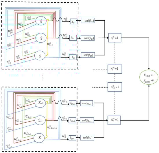
Figure 1.
Schematic diagram for DHNN-L3SAT.
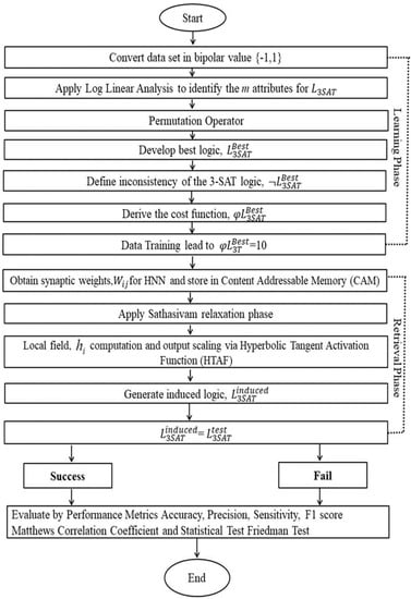
Figure 2.
Flow chart of the workflow of .
The methodology used in this study is illustrated in Figure 2 and comprises a logic phase and a training phase. The flow chart shows that the pre-processing method is involved in the learning phase, making it a critical step. Therefore, the quality and appropriateness of the pre-processing method can significantly influence the performance of the logic mining model. To evaluate the performance of the induced logic after completing the training phase, performance metrics were utilized. These metrics were used to determine whether the model accurately predicted the outcome or if it required improvement.
5. Proposed Higher-Order Log-Linear Model in Logic Mining
This paper discusses the method of a higher-order log-linear analysis and the objective function of a multi-unit DHNN. The following section explores the formulation of a log-linear model, including the selection of significant attributes, and the creation of a multi-unit DHNN. Furthermore, in each section, the log-linear formula is well explained according to the objective function.
5.1. Log-Linear Analysis to Represent 3-Satisfiability Logic
One of the significant applications of logic in DHNN is logic mining. Logic mining is used to extract logical rules from real-life datasets. Logic mining is different from data mining methods in the literature [23,24,25,26,27,28,29,30,31] because the end product for logic mining is a classification model based on SAT rules. The main goal of logic mining is to extract a logical rule that explains the behavior of the dataset. Note that logic mining that utilizes 3SAT in a DHNN was first proposed by Zamri et al. [25] and can be abbreviated as 3SATRA. In this context, it is imperative for logic mining to have a more effective DHNN model that is governed by higher-order logic. However, a real-life dataset might consist of hundreds of attributes and often contributes to the “curse of dimensionality” [32] in logic mining. One of the possible solutions to this problem is choosing the right attribute to be processed by logic mining.
One of the possible methods of extracting the right attributes is through a log-linear analysis. In this paper, we propose a log-linear analysis using 3SATRA or . Let N be the quantity of variables that represents the attribute in bipolar form . Before proceeding to the DHNN, we are required to extract the best attributes from the total of from the datasets. The log-linear model is used to examine whether there is a significant difference between the proportion of categories with two or more group variables [33]. This model expresses the log of an expected frequency in a contingency table as a summation of the function for all parameters involved in the datasets. Note that the two-way table with respect to the expected frequency, , for a column is given as follows if each of the neurons is independent from each other [34].
where n is the sum of entries, while and stand for partial distributions for the variables in the i-th row (row probabilities) and j-th column (column probabilities), respectively. The outcome of performing a linear regression on Equation (15) is shown in Equation (16):
The frequency for the cross-tabulation cell is predicted using a linear model for the log-linear function. The margins and interaction between the variables should be measured in a two-way table known as a saturated model. Equation (17) shows the formulation for the saturation model:
where ρ = ln n is the true outcomes, while are the basic outcomes of neurons and , respectively. According to [29], the association parameter that represents the ability to adapt the log expected cell frequency is expressed using only the partial distribution of each variable and . Equation (18) reproduces the observed frequencies perfectly, known as a saturated model. G2 and the Pearson chi square are used to evaluate the goodness of fit to acquire the likelihood ratio.
Equations (18) and (19) are employed to identify the results based on both the statistical sample size and targeted model [35]. Additionally, the values of these two statistics are computationally the same. In the log-linear analysis, determination of the significance level requires assessing both the parameter and the goodness of fit. In model, the significance of the parameters is evaluated using a partial association test, which calculates the difference in values for the relevant degrees of freedom (df) in the model. Essentially, this means that if there is a relationship between a pair of variables, the null hypothesis test can be selected [36]. Additionally, the null hypothesis is rejected when the parameter values of each individual variable are found to be significantly associated. The alternative hypothesis assumes that there is a significant difference between the observed data and the population parameter. In hypothesis testing, the goal is to reject the null hypothesis in favor of the alternative hypothesis based on statistical evidence [37]. The outcomes of the variables are shown by the generated parameter, by indicating the both values. is then embedded into the DHNN and can be formulated using the values, whereas are significant p-values for attributes , respectively. Additionally, represents the lowest significant p-value between . To guarantee the final model of L3SAT, this work implemented a log-linear analysis and embedded it into a DHNN model according to [38]. It is important to note that neither neuron was considered in the L3SAT formulation when evaluating the performance of each neuron. Another consideration in this suggested method is the changes in traditional k-SATRA proposed by [24,25] if Equation (20) for all variables cannot reach the threshold variable when . Furthermore, determining the neuron negativity presents the biggest problem in Equation (15). The essence of a log-linear analysis is to remove any weak neurons, as indicated by Equations (18) and (19). In this study, we apply a log-linear analysis in the 3-satisfiability-based reverse analysis multi-unit approach or in order to determine which attributes in the dataset will be selected to represent specific variables in the . In particular, utilizes a log-linear analysis to select the best nine attributes that have the strongest interactions among the dataset outcomes. To apply higher-order logic, the selected nine attributes are randomly permuted. The selected ideal attribute will then be represented as an induced logic in the form of a 3SAT, which will be embedded into the DHNN. This method was also implemented by [30], in work on the 2SAT logical rule based on a six-attribute selection. This method obtains the optimal solution when we compare the logic mining method introduced by [30] with 2SAT logical rules.
5.2. New Objective Function with Multi-Unit DHNN
In previous studies, such as [24,25,26,27,28,29], the objective function of the pre-processing phase is to find the best logic that maximizes the true positive . After obtaining the most optimal , the DHNN will learn this logic and obtain the optimal synaptic weight, which leads to the final induced logic. The main issue with this procedure is the lack of consideration of another important variable, which is the true negative . A previous study [39] failed to consider the , which plays a pivotal role in obtaining a negative variable in the induced logic. In this paper, we propose a new objective function that considers and maximizes the summation of and . The formulation of the objective function is as follows:
where is the cardinality of TP in set that has a state equal to 1. Note that represents the DHNN unit. In other words, represents the initial behavior of the dataset before being learned by the DHNN. Equation (20) is different from the work by Zamri et al. [25], where only with the highest frequency was chosen. In this paper, the top logic that satisfies the condition in Equation (20) is chosen to proceed to the learning phase.
5.3. in Multi-Unit DHNN
The next strategy to learn through the DHNN is proposing a multi-unit DHNN that processes several independently. This strategy ensures that the proposed can cover more search space during the retrieval phase. This can be implemented by capitalizing on the synaptic weight from different types of , which leads to different directions in the final neuron state. Kasihmuddin et al. [18] proposed a mutation DHNN to address a similar concern by increasing the search space by mutating the final neuron state. However, due to the limited number of synaptic weights produced by the Wan Abdullah method, the final neuron state tends to converge towards a similar neuron state. From this perspective, we can obtain different types of final neuron states just by obtaining different logic during the learning phase of the DHNN [40]. The equation that governs the multi-unit DHNN is given as follows:
where refers to a multi-unit DHNN in which the structure leads to . After obtaining a satisfactory interpretation, the synaptic weight of can be obtained and is stored as CAM in each multi-unit DHNN. During the retrieval phase of the DHNN, the final neuron state is obtained using Equation (9) and is transformed into the following induced logic.
Next, using the obtained induced logic, the outcome of the induced logic is compared with the testing data. In this context, the comparison is only made with all of the proposed from different DHNN units. Algorithm 1 shows the pseudocode of the proposed work.
| Algorithm 1: pseudocode of . |
| Input Set all attributes with respect to GC, and trial Output The best induced logic Begin Initialize algorithm parameters; Define the attribute for with respect to Search the p-value for each Attribute; for (α < p) do if Equation (7) is satisfied then Assign as and continue; while (i ≤ GC) do Using Equation (21) to find the Check the clause satisfaction for Compute using Equation (12) Compute the synaptic weight associated with by using WA approach: Store the synaptic weight and in CAM; Initialize the final neuron state; for (k ≤ trial) Compute using Equation (9); Convert to the logical from using Equation (22); Combine to form induced logic Compare the outcome of the with the continue; - k ← k + 1 end for i← i + 1 end for End |
6. Experimental Setup
To validate the performance of the proposed , the experiment setup must be performed according to the following setup:
6.1. Benchmark Dataset
The for 15 datasets is extracted using the log-linear analysis in Section 5.1. These datasets and their assigned labels are retrieved from the UCI machine learning repository (https://archive.ics.uci.edu/ml/datasets.php) and Kaggle open set (https://www.kaggle.com/datasets). The dataset was downloaded on 6 November 2022 from the respective website. To avoid possible bias, we chose datasets from different fields of studies (refer to Table 1). Table 1 shows the details of each selected dataset.

Table 1.
Details of each selected dataset.
There are two main criteria for choosing datasets. First, each dataset must contain at least 15 attributes. This is important for validating the capability of the log-linear model in extracting the best attributes during the pre-processing phase. In other words, if we choose datasets that have less than 10 attributes, the proposed model would provide the same results as the work by Zamri et al. [25]. Second, the number of instances must be more than 200 to avoid overfitting in . When the number of instance is very low, there is a high chance that the learning data will consist only of and , which leads to random selection. In addition, k-means clustering [30] will be used to convert the value of the dataset into bipolar form . This conversion is crucial to ensure that the proposed can be compared with other existing work. Since each attribute is represented in bipolar form, the missing data are assigned randomly to 1 or −1. According to Sathasivam [38], the CAM dismisses the outlier data in the bipolar form as being the fault tolerance of the DHNN.
The continuous attribute values in the dataset are standardized using k-means clustering by converting them into bipolar representations. The method used for k-means clustering was inspired by the work of [24,25,31]. To address the issue of missing values, they are replaced with a random bipolar state (either 1 or −1), but the selected datasets should have very few missing values to ensure that the learning phase is not affected.
In addition, all simulations utilize the train-split [30] method, where the training phase contains 60% of instances and the testing phase contains 40% of instances. This method has been used in various studies [24,25,26,27,28,29,30,31], where a further testing percentage was used to confirm the effectiveness of the . This study used k cross validation on the limited sampling instances to estimate how the dataset is expected to perform in the testing phase; those same instances are not used during the training phase for the model.
6.2. Performance Metrics
Based on popular classification metrics such as accuracy (Acc), precision (PREC), sensitivity (SEN), F1 score (F1), and Matthews correlation coefficient (MCC), the effectiveness of the suggested model can be assessed. Acc is applied to figure out the percentage of true-positive and true-negative predictions over the total number of instances. The numbers of instances accurately anticipated a positive and negative cases are known as the true positive (TP) and true negative (TN), respectively, whereas false-positive (FP) and false negative (FN) instances are the sum of the number of falsely anticipated negative and positive outcomes, respectively. The Acc value can be measured using Equation (23), as shown in [41]:
SEN examines the positive tendencies of the instances accurately anticipated in a particular situation, as mentioned by [42].
According to [43], PREC is used to analyze the number of positive outcomes among the false-positive outcomes from the predicted outcomes. The PREC can be formulated as follows:
F1 is also one of the metrics used to measure accuracy. F1 is the modulation index of the sensitivity and precision parameters. The F1 formula is presented in the following equation:
The effectiveness of the logic mining process is evaluated in the Matthews correlation coefficient (MCC), which considers all the elements of a confusion matrix. According to [44], MCC is a valid indicator for evaluating the quality of the proposed model and may be applied in various sizes of classes.
6.3. Baseline Methods
The performance of the model is compared with numerous well-known current works to confirm the efficiency of the suggested methodology. Even though there are numerous classification algorithms that have been introduced, including those proposed by [43,44,45,46,47], none of these studies have demonstrated that induced logical rules can effectively categorize and extract patterns from a dataset.. Note that the authors of [48] have proposed logic mining that utilizes a log-linear model, but the order of the logic is lower than what we propose in this paper. In addition, our proposed model is incomparable with the work in [49] due to the structure of the radial basis function neural network (RBFNN), which only produced a single . Thus, our proposed model is compared with the following state-of-the-art logic mining methods:
- (a)
- 2SATRA [24] was the first attempt at extracting the best from datasets. This logic mining method utilizes systematic as a logical rule during training and testing phase. As for the preprocessing phase, 2SATRA uses random selection to choose the best attribute. In terms of the best logic , 2SATRA uses the objective function that maximizes the number of . In addition, 2SATRA only uses a single-unit DHNN.
- (b)
- E2SATRA [27] utilizes energy-based logic mining to ensure that the always follows the dynamic of the Lyapunov function. During the retrieval phase of the DHNN, the neuron state that achieves the local minimum energy is discarded. In this context, the number of is theoretically lower than those of 2SATRA and P2SATRA. E2SATRA uses similar objective functions to that of 2SATRA and only utilizes a single-unit DHNN.
- (c)
- L2SATRA was inspired by the work of [50], which employed the log-linear method to extract a model for an ovarian cyst dataset. This standard selection method utilized characteristics and incorporated conventional 2SATRA based on a log-linear analysis. Although the log-linear method was utilized to extract the best attributes, L2SATRA does not contain a permutation operator. L2SATRA uses a similar objective function to that of 2SATRA and only utilizes a single-unit DHNN.
- (d)
- P2SATRA [26] is an extension of the work by [51], where was formulated with a permutation operator and took into consideration various configurations for the literals in . The permutation operator determines all the possibility search spaces of the and leads to the highest accuracy value. P2SATRA uses similar objective functions to that of 2SATRA and only utilizes a single-unit DHNN.
- (e)
- RA [23] is the earliest logic mining that utilizes HornSAT when extracting a logical rule from a dataset. The initial RA does not contain any pre-processing phases and generalized induced logic. In this paper, the RA is the systematic second-order logic during the preprocessing phase. During the retrieval phase, only a that has the property of HornSAT is chosen. RA uses a similar objective function to that of 2SATRA and only utilizes a single-unit DHNN.
- (f)
- A2SATRA was inspired by [30], and its permutation operator investigates every conceivable search space that is connected only to the selected attributes. Attributes are selected by focusing only on a log-linear analysis by selecting significant attributes in the form of a contingency table. In the context of the learning and testing phases, A2SATRA uses a similar objective function to that of 2SATRA and only utilizes a single-unit DHNN.
6.4. Configuration Model
The configuration model of was built based on a log-linear analysis, which consists of a multidimensional examination dataset in the form of a contingency table that presents the relationship between the qualitative and discrete scales. However, concentrates on only one-way interactions to identify the minor qualities that could potentially cause the logic to overfit. Equation (16) is used to measure the likelihood ratio to detect any significant effects and to carry out a primary interaction analysis. Significant attributes are determined using Equation (18) and the permutation attributes are determined using Equation (19). The permutation operator in Equation (20) is used to expose all the interconnections among the variables of . Equation (21) determines the significant attribute applied. We incorporate the configuration of the into DHNN-3SAT using the optimal attribute which leads to via Equation (2).
Table 2 shows the k-Way model and higher-order effects component for , whereby the saturated model yields the significant effect components. We want to understand how the variables interact with one another rather than with all the attributes; hence, is the most important value to observe how using into DHNN can create interactions between variables by concentrating just on one specific variable at a time. Due to the p-value of the Pearson chi square being less than 0.05, it is possible to infer that the number of iterations representing the trial variable stops at one point significantly more often than expected by chance. Table 2 shows that the first-order effects have a substantial impact on the model. Even though in Table 2 it was indicated that the first-order effect had a significant impact on the analysis, we still need to consider partial relationships among all the variables. As a result, to obtain the partial association findings, the variables selected before being expressing in the 3SAT logical structure are analyzed. The parameters are selected based on the p-value by excluding unimportant qualities from the datasets .
Table 2.
Contingency table with significant values.
6.5. Experimental Design
In this experiment, we used IBM SPSS Statistics version 27 to perform a log-linear analysis on each dataset in Table 1. The specific concentrations used are listed in Table 3, which provides a comprehensive overview of the experimental parameters and their respective values. We used cross-validation to identify the most important attribute, which we then used for logic mining in DEV C++ Version 5.11. The simulation ran on a device with an AMD Ryzen 5 3500U processor, Radeon Vega Mobile Gfx, and 8 GB of RAM running on Windows 10. To ensure consistent results, we ran all trials on the same device to avoid any potential errors during the simulation.
Table 3.
The parameters for each standard logic mining method.
7. Results and Discussion
The primary aim of this study is to assess the performance of logic mining when using a pre-processing structure to select attributes. In this section, we evaluate its performance by comparing with existing work. The results of each performance metric for (the existing logic mining = ), where + is the existing logic mining loss in and - is the existing surplus by , compared with existing methods, showed good results and are discussed in this section.
7.1. Accuracy for Current and Logic Mining Models
Table 4 shows the ACC results for the selected logic mining model. There are several variations in the performances for . The bold values indicate that the logic mining method achieved the maximum value. Diff refers to the differences between the proposed logic mining method () and the selected existing logic mining method. Table 4 also displays the average value and minimum, maximum, and average ranks of the Friedman test. The accuracy values were recorded following computing using Equation (23).
Table 4.
Acc value for in comparison with state-of-the-art logic mining methods.
- (a)
- Several decent performances resulted from the . The application of the log-linear analysis is assumed to be highly effective in pre-processing methods, as it identifies significant attributes with a p-value of p ≤ 0.05. This results in optimal synaptic weight values associated with the resulting attributes for L3SAT [50]. Furthermore, since the logical rules embedded in the model are well-structured, the outcomes have the potential to achieve higher values for the true positives (TPs) and true negatives (TNs).
- (b)
- The dataset L11 (Facebook Metric) was significant because its accuracy rating was almost 1. Therefore, we can conclude that the induced logic obtained an accuracy that was very close to 1 for all TP and TN. However, a study by [26] found that, when compared with the log-linear integration method using the nine-attribute permutation method, the P2SATRA method with restrictions improved identification of the best induced logic and produced more satisfactory results based on true data. This indicates that, in terms of the performance of the dataset, the local field can extract the best induced logic [54].
- (c)
- According to Table 4, there are several values for our proposed logic in which an accuracy of Acc > 0.8 was achieved. Therefore, we can deduce that the proposed logic mining method separate true positives from true negative for datasets. Therefore, our work applied Wan Abdullah’s approach to obtain optimal synaptic weight stands [17] to decrease the false negative values that can be produced in clauses [23].
- (d)
- The induced logic retrieved for L8 is . L8 refers to symptoms of hepatis disorder, with attribute A, B, C, D, E, F, G, H, and I representing steroid, antivirals, fatigue, malaise, anorexia, liver big, liver firm, spleen palpable, ascites, and varices, respectively. According to the induced logic, the symptoms of hepatis disorder increase when bilirubin increases by about 60% for factors A, C, E, and G.
- (e)
- The Friedman rank test was performed on each dataset with and degree of freedom . The Acc p-value is less than 0.05 . The null hypothesis, which claimed that all logic mining models perform identically, was rejected. As mentioned by [30], the highest average rank is evidence of the superior performance of a logic mining model. In this research, the proposed model achieved a mean rank of approximately 1.6 among the other logic mining models. However, the second-highest rank was achieved by P2SATRA [21], which closely competed with our model, with an average rank of approximately 2.23.
As shown in Figure 3, we can conclude that the high ACC value is due to the effective training phase, which leads to an optimal synaptic weight for the 3SAT logical rule. This enables the network to retrieve the optimal induced logic through a local field (Equation (9)). By using a log-linear analysis to select the best attribute, we can further improve the accuracy by obtaining optimal synaptic weights, which leads to higher true positive (TP) and true negative (TN) values. Additionally, the log-linear model can eliminate non-significant attributes, resulting in lower false positive (FP) and false negative (FN) values. Comparing our work with RA(HornSAT) [18], we observe that the non-flexible synaptic weight of their logical structure results in lower TP and TN values. The suboptimal synaptic weight also leads to suboptimal induced P, which is further exacerbated when attributes are randomly selected in RA(HornSAT). This feature contributes to the lower TP and TN values in RA(HornSAT).
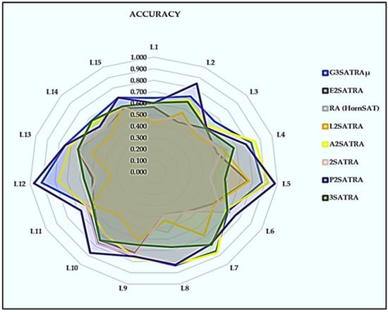
Figure 3.
Accuracy of logic mining models.
7.2. Precision for Current and Logic Mining Models
The PREC values for the chosen logic mining model are displayed in Table 5 below. shows several variations in performance for each dataset. The values in bold show that the specific logic mining method reached its maximum value. Diff denotes the differences between the chosen current logic mining and the proposed logic mining (). Table 5 also shows the Friedman test’s average value, minimum and maximum ranks, and range for ranks. The precision values here were predicated based on Equation (25).
Table 5.
PREC value for in comparison with state-of-the-art logic mining methods.
- (a)
- PREC shows that performs better than other logic mining models across all 15 datasets. This demonstrates the capability of to extract a high value for true positives. improved the performance of the 3SATRA proposed by [20] by embedding optimal attributes in the 3SAT and retrieving optimally induced logic that is important to the dataset. As a result, is more capable than other current logic mining models at producing successful outcomes.
- (b)
- achieved a PREC that is very close to 1 (Precision = 1) in two datasets, L5 and L6. There, it shows that the induced retrieved by can predict positive outcomes with certainty. Every dataset output from the induced equals 1. The proposed logic mining model yields a precision that is almost equal to 1 in datasets L5 and L6. Therefore, the final neuron states obtained from the local field provide a satisfactory interpretation as a result [25].
- (c)
- In comparison with A2SATRA proposed by [30], the proposed in this paper is able to more accurately predict positive instances, with the exception of three datasets (L4, L6, and L7). While P2SATRA suggested by [21] may still predict the best induced logic for five datasets (L2, L5, L10, L12, and L13), the model can achieve higher positive values for these specific datasets.
- (d)
- This proposed model outperforms other logic mining models such as E2SATRA, RA, 2SATRA, 3SATRA, and L2SATRA in terms of achieving higher values of true positives (TPs) and true negatives (TNs). It has been demonstrated that using a log-linear analysis for attribute selection and multi-unit theory in 3SAT leads to more accurate TP values.
- (e)
- The average rank of the proposed logic mining model is 1.600, which is higher than the average rank of other models. The closest competing method is P2SATRA, with an average rank of 2.530. The statistical analysis confirms that our proposed model is superior to the other methods. This means that our model is very good at identifying both positive and negative results.
In Figure 4, the precision value is higher compared with other existing logic mining methods such as RA(HornSAT), E2STRA, 2SATRA, and A2SATRA. The proposed model using a log-linear analysis achieved a higher Pbest value by selecting the perfect attribute from the whole dataset. The permutation operated within a very large searching space to reduce the cost function. The multidimensional solution in the proposed systematic logical structure led to obtaining more TNs and less FPs. The existing logic mining methods L2SATRA [50] and A2SATRA [30] obtained sup-optimal performances in the testing phase, obtaining more FPs that reduce the precision value for their model.
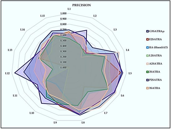
Figure 4.
Precision of logic mining models.
7.3. Sensitivity for Current and Logic Mining Models
Table 6 shows the SEN results for the selected logic mining model. There are variations in the performances of the . Whereas the bold values indicate that the particular logic mining achieved the maximum value, diff refers to the differences between the proposed logic mining method () and the selected existing logic mining method. Table 6 also displays the average value and minimum, maximum, and average ranks from the Friedman test. These SEN values were obtained using Equation (24).
Table 6.
SEN values for in comparison with state-of-the-art logic mining methods.
- (a)
- Our proposed logic mining method outperformed the 3SATRA and P2SATRA. This demonstrates the importance of the log-linear-approach-chosen features for a given dataset not being significant for the dataset. The random selection proposed by [26] successfully retrieved for all outcomes.
- (b)
- Our model achieved a SEN close to 1 (0.937), indicating its ability to predict positive outcomes in the retrieval phase of the DHNN for the L5 dataset. For the other datasets, our model demonstrated high TN and TP values compared with other logic mining models. In fact, for the L7 and L8 datasets, our proposed model achieved higher TN and TP values than other models.
- (c)
- There are some instances where the sensitivity was not recorded due to the lack of a positive outcome for that dataset in the logic mining methods E2SATRA and L2SATRA. Furthermore, there is a good likelihood that the dataset represents an actual situation and that the testing data only contains negative classes. It follows that the induced is bias towards to the negative class.
- (d)
- For all of the datasets, the Friedman rank test was performed with and . The p-value for Sen is <0.05, and . As a result, the null hypothesis that all logic mining models perform equally well was rejected. According to Table 6, ’s performance still displays a competitive Sen value when compared with other published work such as 3SATRA, P2SATRA, and A2SATRA. The lowest statistical average rank achieved in the logic mining method E2SATRA was 5.80. This statical test can predict that A3SATRA can still reach the when adding another optimization layer, which would increase the DHNN’s complexity.
Similarly, to the precision metrics, the confusion metric for sensitivity also achieves a higher TP value in the proposed logical structure when compared with other logical structures, except P2SATRA [26]. Figure 5 shows the selection of random attributes and the permutation operator obtaining an accurate local field to achieve the best optimal solution. The is not bad in terms of the optimal solution when we used the Friedman rank test. Its ranking value was still of a higher order compared with the other current logic mining methods.
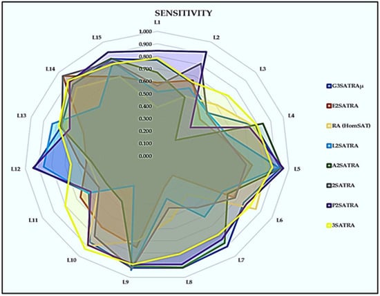
Figure 5.
Sensitivity of logic mining models.
7.4. F1 for Current and Logic Mining Models
Table 7 shows the F1 result for the selected logic mining model. There is variation in the performances for the . Whereas the bold values indicate that the particular logic mining method achieved the maximum value, diff refers to the differences between the proposed logic mining method () and the selected existing logic mining method. Table 7 also displays the average value and minimum, maximum, and average ranks from the Friedman test. These F1 values were computed using Equation (26).
Table 7.
FI value for in comparison with state-of-the-art logic mining methods.
- (a)
- The multi-unit forms quite a good number of positive outcomes when learning from all the datasets [41]. When we compare P2SATRA with the proposed , performance is lacking in terms of retrieved positive outcomes. Therefore, the authors of [29] stated that the optimal value for synaptic weight is kept in the content addressable memory, and can enhance the local field when computing the ideal final neuron state.
- (b)
- One dataset, L5, obtained an F1 score of 0.921, which is close to 1, in the proposed model . This shows that our proposed produced the correct number of TPs during the retrieval phase of the DHNN, and as we know through previous work [43], if F1=1, the model has perfect precision and recall (correct positive predictions relative to total actual positives) efficiency.
- (c)
- There is no instance where our data return an F1 score = 0; therefore, our proposed logic was able to produce TPs. The that was determined by computing the local field is sensitive to correctly forecasted positive situations. The majority of leaned towards = 1, reaching the value of F1. The induced logic led to
- (d)
- All datasets with and seven degrees of freedom underwent the Friedman test accurately. The F1 p-value is , and . Thus, the null hypothesis that all logic mining models will perform equally well was rejected. However, compared with the other works, obtained a great average rank equal to 1.53. This is the outcome of ’s ability to anticipate which attributes maximise TP during the DHNN retrieval phase.
In Figure 6, we continue analyzing the FI value with all of the higher-order logical structures; 3SAT has a higher probability of being a satisfied logic. Its higher-order logical rule obtains the correct synaptic weight to achieve an ideal local field, which increases accuracy. is still has the highest FI value compared to other logic mining methods, which are second-order logical structures with a high probability of being an unsatisfied condition. A successfully selected random attribute obtains more FP values in the 15 selected datasets. As we can see, the 3SATRA proposed by [25] still can achieve an optimal value close to that of due to both being higher-order logical structures.
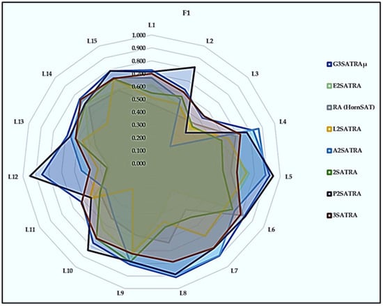
Figure 6.
FI Score of logic mining models.
In Figure 6, we continue analyzing the FI value with all of the higher order logical structures; 3SAT has a higher probability of being a satisfied logic. It higher-order logical rule obtain the correct synaptic weight to achieve an ideal local field, which increases its accuracy. is still in the lead in terms of FI value compared with the other logic mining methods that are second-order logical structures with very high chances of being an unsatisfied condition. A successfully selected random attribute obtains more FP values in the 15 selected datasets. As we can see, the 3SATRA proposed by [25] can still achieve an optimal value close to that of due to both being higher-order logical structures.
7.5. Matthews Correlation Coefficient for Current and G3SATRAµ Logic Mining Models
The MCC result for the chosen logic mining model can be seen in Table 8. displays a variety of linear capabilities. The bold numbers, on the other hand, show that a given logic mining approach has reached its maximum value. Diff represents the differences between the chosen existing logic mining method and the suggested logic mining method (). The average value and minimum, maximum, and average ranks of the Friedman test are shown in Table 8. These MCC values were obtained using Equation (27).
Table 8.
MCC value for in comparison with state-of-the-art logic mining methods.
- (a)
- Our proposed logic mining method, the multi-unit , managed to obtain optimal results for MCC, about 10 out of 15, for all datasets. The authors of [51] mentioned that as the MCC value approaches 0, the values are able to predict which attributes will be randomly selected. In this aspect, the MCC value analysis assists in determining the effectiveness of the confusion matrix derived from the induced logic extracted by .
- (b)
- The log-linear analysis proposed by [30] is able to produce the best attribute selection in A2SATRA and to obtain instances of positive outcomes, with MCC = > 0.5 in this research analysis. As a result, the MCC values of the five datasets in the model are more than 0.5 among the 15 dataset (L4, L7, L9, L10, and L12).
- (c)
- Datasets L5 and L6 obtained values of zero, as the MCC was not registered because no positive outcome was registered throughout the dataset. This indicates in the model, is not reliable. In some the other logic mining methods, the false values of zero in logic mining methods E2SATRA, L2SATRA, and 2SATRA are not reliable in certain datasets.
- (d)
- All datasets with α = 0.05 and df= 7 were subjected to a Friedman rank test. The MCC p-value is , and . As a result, the null hypothesis that all logic mining models perform equally well was rejected. The highest average rank among the currently used methods is 1.87, for . At the same time, notice that P2SATRA, with an average rank of 2.800, is the method that most closely rivals . As a result, it indicates that all the confusion matrices proposed in this study statistically support ’s superiority over those in previous studies.
According to the findings in Figure 7, has a greater MCC value than the other available methods. This model capitalizes on higher-order k-satisfiability logic as opposed to the model put forth by [26], where only second-order logic was used to represent the dataset. Throughout this condition, has a greater logical capacity to reflect the dataset’s dimensionality. The proposed log-linear analysis in Equation (20) can filter a greater number of non-significant attributes using higher values of k, which results in well-balanced TPs and TNs. For learning in the HNN, additionally obtains more than one , preventing the network from becoming overfit with a single . As a result, the in the has a greater MCC value, preventing it from becoming a random classifier. E2SATRA was found to have several drawbacks E2SATRA uses 2SAT poor capacity in a satisfied logical rule. The lower-order logical structure retrieves worse CAM than higher-order logic, which can minimize the energy (). significantly achieves a smaller search space. There is a higher chance that only one induced logic was discovered during the learning phase, which caused the MCC value to be close to zero, converging to the random classifier.
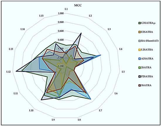
Figure 7.
MCC of logic mining models.
From Figure 8, we can conclude that the Friedman test is a statistical test that does not rely on specific assumptions about the data, and it is commonly used to compare three or more related groups or conditions. This test is preferred when the data do not meet the criteria needed for parametric tests, such as a normal distribution or homogeneity of variances. In the Friedman test, the highest rank refers to the logic mining method with the highest median rank across all the logic mining included in the study, which indicates that it performed the best or had the most favorable outcome compared with all the other logic mining methods compared. Similarly, the lower ranking is a crucial element in interpreting the results of the Friedman test as it helps to identify which treatment or condition performed the worst and suggests that it may require improvement or elimination in future studies.
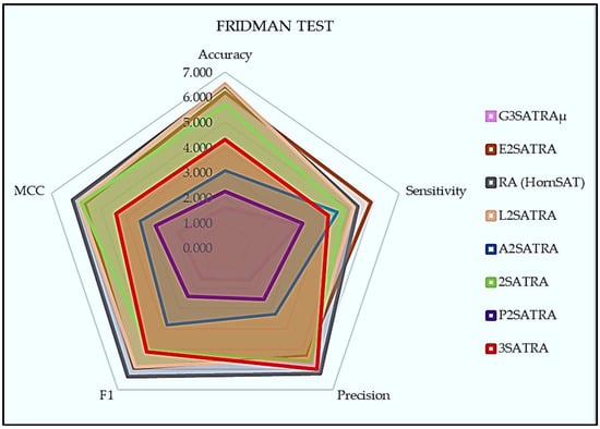
Figure 8.
Friedman test results for logic mining models.
According to the results of the test, the model achieved the highest average rank among all the logic mining models that were discussed. This means that the model performed better than the other models. The second highest average rank among the logic mining models was achieved by the P2SATRA model. The permutation operator used in the P2SATRA model had a significant impact on its performance during the statistical test. Overall, the results of the Friedman test indicate that the model is the best performing logic mining model among those evaluated. However, it is important to note that the test only evaluated a specific set of models and may not necessarily generalize to other models or scenarios. In contrast, the RA(HornSAT) achieved the lowest rank in a Friedman test result. This indicates that it had the lowest median rank among all the proposed logic mining approaches in the study and performed the worst or had the least favorable outcome among all the logic mining methods compared.
In summary, the proposed logical structure demonstrates superior performance compared with other logic mining methods, according to the technical analysis. The uses a log-linear analysis to select the best attributes, which results in optimal synaptic weights, leading to higher true positives and true negatives and lower false positives and false negatives. The different performance metrics such as accuracy, precision, sensitivity, MCC, and F1 score showed that the proposed method outperforms the other logical mining methods, except for P2SATRA in sensitivity, which achieved more true positives. Additionally, the statistical test results ranked the proposed method as the best among the other methods. The goal of this study was to assess the effectiveness of the proposed method relative to other logic mining techniques using a range of performance metrics and statistical tests. This evaluation aimed to determine whether the proposed method performs better than other methods and, if so, to what degree.
8. Limitation of
The aim of logic mining is to extract rules and patterns from data that can be used to make predictions or to gain insights into the underlying structure of the data. However, like any other scientific method, logic mining has its limitations. There may be cases where the data are too noisy or where the patterns are too complex for the method to effectively identify useful rules. There may also be situations where the method is too computationally expensive or requires too much data to be practical.
Therefore, in this study, we aim to explore these limitations in more detail. By identifying and understanding the limitations of logic mining, we can find ways to enhance the effectiveness of logic mining techniques.
- (a)
- Only focusing the log-linear approach on selecting significant attributes. Firstly, by removing insignificant attributes from the dataset before translation into higher-order logical rules, the complexity of the logic mining process can be reduced, which can lead to a faster and more efficient model in the training phase. The selected attribute that best represents the dataset can improve the overall accuracy and performance of the logic mining model and can reduce the risk of overfitting, which can improve the generalizability and applicability of the .
- (b)
- Selecting multi-unit optimal 3-satisfiability logical rules is dependent on the selection of true positive and true negative values. Relying on a single set of values for true positives and true negatives may not be sufficient in capturing the intricacies of the dataset, thus resulting in suboptimal solutions. However, using multi-unit optimal logical rules may lead to a substantial expansion of the search space for the discrete Hopfield neural network, particularly when dealing with highly complex or noisy datasets.
- (c)
- The multi-unit discrete Hopfield neural network may not always be effective in learning and deriving the best logic from the dataset. The accuracy and performance of the network may be affected by the quality and quantity of the data used in the analysis. Therefore, the use of Wan Abdullah’s method to derive synaptic weights can be effective for highly complex or noisy datasets. Using a multi-unit neural network, the amount of induced logic that represents the behavior of the datasets increases.
- (d)
- The proposed permutation operator for 3-satisfiability logic in a discrete Hopfield neural network enables the identification of the optimal attribute configuration for each logical clause, which can lead to the generation of more accurate and efficient induced logic. Additionally, the use of permutation provides flexibility in the identification of the highest performing induced logic in terms of a confusion matrix, which can improve the overall accuracy and performance of the model. Moreover, the ability to identify the highest performing induced logic through permutation enables the selection of the most relevant and significant attributes, which can lead to more meaningful and interpretable results.
9. Future Work
In selecting a network for our needs, we opted for DHNN over RBFNN and others due to the need for an additional optimization layer when adjusting parameters. The RBFNN requires multiple training phases (no-training, half-training, and full training) to evaluate relevant parameters such as width and center. Even with the right parameters, the feedforward RBFNN only creates a single piece of induced logic, which is usually a simplified linear classifier with no utility. However, this work does not compare DHNN options, such as the one presented by [48]. Instead, this experiment examines the impact of attribute selection on logic mining. It is important to note that in the method, the interaction indicated by a log-linear analysis only depends on the integration of the attributes and the solution. The method is biologically inspired and based on the premise that the human brain is effective at removing unwanted details when the outcome is visible.
Selecting true positive and true negative values from the performance of the logic mining and discrete Hopfield neural network involves experimenting with various selection strategies, such as using different thresholds or weights for each value and evaluating their impact on the quality of the induced logics and the overall performance of the network [55,56]. Another idea could be to explore the use of other machine learning techniques in conjunction with the proposed hybrid logic mining approach, such as deep learning or reinforcement learning. This could involve investigating how these techniques can be integrated with the discrete Hopfield neural network to further enhance the accuracy and efficiency of the logic mining process, particularly when dealing with large and complex datasets. Finally, other potential studies can apply the proposed hybrid logic mining method to specific real-world problems or applications, such as fraud detection or medical diagnoses. This could involve adapting the approach to the specific requirements and characteristics of the problem domain and evaluating its performance and effectiveness in comparison with existing solutions.
10. Conclusions
In this paper, we proposed a new logic mining that utilizes several fresh perspectives. First, we formulated a log-linear approach by selecting significant higher-order attributes with respect to the final logical outcome. Using this approach, we reduced the number of insignificant attributes in the datasets. Second, a new objective function that utilizes both true positives and negatives during the pre-processing phase was proposed. The new objective function considers negative outcomes, which were not considered in previous state-of-the-art methods. Third, this paper proposed the first multi-unit DHNN where each unit learns from individual , which leads to diversification of the induced logic. Fourth, the proposed logic mining in this paper utilizes a permutation operator to ensure the optimal arrangement of the attribute was used during the learning phase of a DHNN. Finally, extensive experimentation using various real-life datasets was performed in and was compared with other state-of-the-art logic mining methods. Based on these results, our proposed was observed to outperform the state-of-the-art logic mining methods in terms of various performance metrics and statistical validation. Ultimately, this signifies the robustness of the in extracting the most optimal logical rule. As for future work, the proposed can be implemented using non-satisfiable logic such as maximum satisfiability. This study provides a new perspective in extracting datasets that have negative outcomes in nature. In addition, metaheuristics algorithms such as reinforcement learning and simulated annealing can be implemented during the learning phase of a DHNN to ensure only that correct synaptic weights are obtained.
Author Contributions
Conceptualization, methodology, software, writing—original draft preparation, G.M.; formal analysis; S.N.F.M.A.A.; validation, N.‘A.R.; supervision and funding acquisition, M.S.M.K.; writing—review and editing, S.A.; visualization, N.‘A.R.; project administration, M.A.M. All authors have read and agreed to the published version of the manuscript.
Funding
This research is fully funded and supported by Universiti Sains Malaysia, Short Term Grant, 304/PMATHS/6315655.
Data Availability Statement
Not applicable.
Acknowledgments
The authors express special thanks to all researchers in the Artificial Intelligence Research Development Group (AIRDG) for their continued support. We also acknowledge “Universiti Sains Malaysia, Short Term Grant, 304/PMATHS/6315655” for the support and funding.
Conflicts of Interest
The authors declare no conflict of interest.
References
- Witten, I.H.; Frank, E. Data mining: Practical machine learning tools and techniques with Java implementations. Acm Sigmod Rec. 2002, 31, 76–77. [Google Scholar] [CrossRef]
- Li, H.; Li, T. A review of data mining techniques and their applications in healthcare. Int. J. Med. Inform. 2022, 158, 104618. [Google Scholar]
- Wu, X.; Zhu, X.; Wu, G.Q.; Ding, W. Data mining with big data. IEEE Trans. Knowl. Data Eng. 2014, 26, 97–107. [Google Scholar]
- Wang, X.; Yao, X.; Sun, Y. Application of data mining techniques in the field of business: A systematic review. Electron. Commer. Res. Appl. 2019, 34, 100827. [Google Scholar]
- Aslani, N.; Galehdar, N.; Garavand, A. A systematic review of data mining applications in kidney transplantation. Inform. Med. Unlock. 2023, 37, 101165. [Google Scholar] [CrossRef]
- Da Silveira Barcellos, D.; de Souza, F.T. Optimization of water quality monitoring programs by data mining. Water Res. 2022, 221, 118805. [Google Scholar] [CrossRef]
- Kaur, J.; Dharni, K. Application and performance of data mining techniques in stock market: A review. Intell. Syst. Account. Financ. Manag. 2022, 29, 219–241. [Google Scholar] [CrossRef]
- Sunhare, P.; Chowdhary, R.R.; Chattopadhyay, M.K. Internet of things and data mining: An application orient-ed survey. J. King Saud Univ. Comput. Inf. Sci. 2022, 34, 3569–3590. [Google Scholar] [CrossRef]
- Miao, F.; Xie, X.; Wu, Y.; Zhao, F. Data Mining and deep learning for predicting the displacement of “Step-like” landslides. Sensors 2022, 22, 481. [Google Scholar] [CrossRef]
- Shafiq, D.A.; Marjani, M.; Habeeb, R.A.A.; Asirvatham, D. Student Retention Using Educational Data Mining and Predictive Analytics: A Systematic Literature Review. IEEE Access 2022, 10, 72480–72503. [Google Scholar] [CrossRef]
- Izonin, I.; Tkachenko, R.; Shakhovska, N.; Ilchyshyn, B.; Singh, K.K. A Two-Step Data Normalization Approach for Improving Classification Accuracy in the Medical Diagnosis Domain. Mathematics 2022, 10, 1942. [Google Scholar] [CrossRef]
- Wang, Y.; Yang, L.; Wu, J.; Song, Z.; Shi, L. Mining Campus Big Data: Prediction of Career Choice Using Interpretable Machine Learning Method. Mathematics 2022, 10, 1289. [Google Scholar] [CrossRef]
- Montisci, A.; Porcu, M.C. A Satellite Data Mining Approach Based on Self-Organized Maps for the Early Warn-ing of Ground Settlements in Urban Areas. Appl. Sci. 2022, 12, 2679. [Google Scholar] [CrossRef]
- Ferandez, D.M.; Cernadas, E.; Barro, S.; Amorim, D. Explainable artificial intelligence (XAI): Concepts, taxonomies, opportunities, and challenges toward responsible AI. Inf. Fusion 2020, 58, 82–115. [Google Scholar]
- Kumar, A.; Tanwar, S. Explainable AI for data-driven decision-making in healthcare. J. Ambient. Intell. Humaniz. Comput. 2021, 2021, 1–13. [Google Scholar]
- Hopfield, J.J.; Tank, D.W. “Neural” computation of decisions in optimization problems. Biol. Cybern. 1985, 52, 141–152. [Google Scholar] [CrossRef]
- Abdullah, W.A.T.W. Logic programming on a neural network. Int. J. Intell. Syst. 1992, 7, 513–519. [Google Scholar] [CrossRef]
- Mohd Kasihmuddin, M.S.; Mansor, M.A.; Md Basir, M.F.; Sathasivam, S. Discrete mutation Hopfield neural network in propositional satisfiability. Mathematics 2019, 7, 1133. [Google Scholar] [CrossRef]
- Sathasivam, S.; Mansor, M.A.; Ismail, A.I.M.; Jamaludin, S.Z.M.; Kasihmuddin, M.S.M.; Mamat, M. Novel random k satisfiability for k ≤ 2 in hopfield neural network. Sains Malays 2020, 49, 2847–2857. [Google Scholar] [CrossRef]
- Zamri, N.E.; Azhar, S.A.; Mansor, M.A.; Alway, A.; Kasihmuddin, M.S.M. Weighted random k satisfiability for k= 1, 2 (r2SAT) in discrete Hopfield neural network. Appl. Soft Comput. 2022, 126, 109312. [Google Scholar] [CrossRef]
- Guo, Y.; Kasihmuddin, M.S.M.; Gao, Y.; Mansor, M.A.; Wahab, H.A.; Zamri, N.E.; Chen, J. YRAN2SAT: A novel flexible random satisfiability logical rule in discrete hopfield neural network. Adv. Eng. Softw. 2022, 171, 103169. [Google Scholar] [CrossRef]
- Mansor, M.A.; Kasihmuddin, M.S.M.; Sathasivam, S. Artificial Immune System Paradigm in the Hopfield Network for 3-Satisfiability Problem. Pertanika J. Sci. Technol. 2017, 25, 1173–1188. [Google Scholar]
- Sathasivam, S.; Wan Abdullah, W.A.T. Logic mining in neural network: Reverse analysis method. Computing 2011, 91, 119–133. [Google Scholar] [CrossRef]
- Kho, L.C.; Kasihmuddin, M.S.M.; Mansor, M.; Sathasivam, S. Logic Mining in League of Legends. Pertanika J. Sci. Technol. 2020, 28, 211–215. [Google Scholar]
- Zamri, N.E.; Mansor, M.A.; Mohd Kasihmuddin, M.S.; Alway, A.; Mohd Jamaludin, S.Z.; Alzaeemi, S.A. Amazon employees resources access data extraction via clonal selection algorithm and logic mining approach. Entropy 2020, 22, 596. [Google Scholar] [CrossRef]
- Jamaludin, S.Z.M.; Mansor, M.A.; Baharum, A.; Kasihmuddin, M.S.M.; Wahab, H.A.; Marsani, M.F. Modified 2 satisfiability reverse analysis method via logical permutation operator. Comput. Mater. Contin. 2023, 74, 2853–2870. [Google Scholar]
- Mohd Jamaludin, S.Z.; Mohd Kasihmuddin, M.S.; Md Ismail, A.I.; Mansor, M.A.; Md Basir, M.F. Energy based logic mining analysis with hopfield neural network for recruitment evaluation. Entropy 2020, 23, 40. [Google Scholar] [CrossRef]
- Li, S.; Li, Y.; Li, R.; Li, X.; Liu, Y. A novel hybrid algorithm for solving large-scale 2-SAT problems. Appl. Soft Comput. 2021, 100, 106997. [Google Scholar]
- Kasihmuddin, M.S.M.; Jamaludin, S.Z.M.; Mansor, M.A.; Wahab, H.A.; Ghadzi, S.M.S. Supervised learning perspective in logic mining. Mathematics 2022, 10, 915. [Google Scholar] [CrossRef]
- Jamaludin, S.Z.M.; Romli, N.A.; Kasihmuddin, M.S.M.; Baharum, A.; Mansor, M.A.; Marsani, M.F. Novel logic mining incorporating log linear approach. J. King Saud Univ. Comput. Inf. Sci. 2022, 34, 9011–9027. [Google Scholar] [CrossRef]
- Alway, A.; Zamri, N.E.; Mohd Kasihmuddin, M.S.; Mansor, A.; Sathasivam, S. Palm Oil Trend Analysis via Logic Mining with Discrete Hopfield Neural Network. Pertanika J. Sci. Technol. 2020, 28, 967–981. [Google Scholar]
- Wu, X.; Zhang, X.; Wei, X. A dynamic Hopfield neural network for constrained optimization problems. Neural Netw. 2017, 87, 43–54. [Google Scholar]
- Cook, S.A. Short propositional formulas represent non-deterministic computations. Inf. Process. Lett. 1988, 26, 269–270. [Google Scholar] [CrossRef]
- Zollanvari, A.; James, A.P.; Sameni, R. A theoretical analysis of the peaking phenomenon in classification. J. Classif. 2020, 37, 421–434. [Google Scholar] [CrossRef]
- Gardini, F.; Trivisano, C.; Lanciotti, R.; Maffei, M.; Guerzoni, M.E. Suitability of log-linear models to evaluate the microbiological quality of baby clams (Chamelea gallina L.) harvested in the Adriatic Sea. Int. J. Food Microbiol. 2000, 54, 63–74. [Google Scholar] [CrossRef] [PubMed]
- Haque, M.M.; Chin, H.C.; Debnath, A.K. An investigation on multi-vehicle motorcycle crashes using log-linear models. Saf. Sci. 2012, 50, 352–362. [Google Scholar] [CrossRef]
- Cumming, G. The new statistics: Why and how. Psychol. Sci. 2014, 25, 7–29. [Google Scholar] [CrossRef]
- Sathasivam, S.; Mamat, M.; Kasihmuddin, M.S.M.; Mansor, M.A. Metaheuristics approach for maximum k satisfiability in restricted neural symbolic integration. Pertanika J. Sci. Technol. 2020, 28, 545–564. [Google Scholar]
- Lloyd, S. Least squares quantization in PCM. IEEE Trans. Inf. Theory 1982, 28, 129–137. [Google Scholar] [CrossRef]
- Sathasivam, S. Upgrading logic programming in Hopfield network. Sains Malays. 2010, 39, 115–118. [Google Scholar]
- Jha, K.; Saha, S. Incorporation of multimodal multi objective optimization in designing a filter-based feature selection technique. Appl. Soft Comput. 2021, 98, 106823. [Google Scholar] [CrossRef]
- Ahmad, S.; Ullah, T.; Ahmad, I.; Al-Sharabi, A.; Ullah, K.; Khan, R.A.; Ali, M.A. Novel hybrid deep learning model for metastatic cancer detection. Comput. Intell. Neurosci. 2022, 2020, 8141530. [Google Scholar] [CrossRef] [PubMed]
- Luque, A.; Carrasco, A.; Martin, A.; Heras, A. The impact of class imbalance in classification performance metrics based on the binary confusion matrix. Pattern Recognit. 2019, 91, 216–231. [Google Scholar] [CrossRef]
- Chicco, D.; Starovoitov, V.; Jurman, G. The benefits of the Matthews correlation coefficient (MCC) over the diagnostic odds ratio (DOR) in binary classification assessment. IEEE Access 2021, 9, 47112–47124. [Google Scholar] [CrossRef]
- Shi, J.; Li, Z.; Zhao, H. Feature Selection via Maximizing Inter-class Independence and Minimizing Intra-class Redundancy for Hierarchical Classification. Inf. Sci. 2023, 626, 1–18. [Google Scholar] [CrossRef]
- Shang, R.; Kong, J.; Wang, L.; Zhang, W.; Wang, C.; Li YJiao, L. Unsupervised feature selection via discrete spectral clustering and feature weights. Neurocomputing 2023, 517, 106–117. [Google Scholar] [CrossRef]
- Wang, P.; Xue, B.; Liang, J.; Zhang, M. Feature Selection Using Diversity-Based Multi-objective Binary Differential Evolution. Inf. Sci. 2023, 626, 586–606. [Google Scholar] [CrossRef]
- Jeon, Y.; Hwang, G. Feature selection with scalable variational gaussian process via sensitivity analysis ased on L2 divergence. Neurocomputing 2023, 518, 577–592. [Google Scholar] [CrossRef]
- Alzaeemi, S.A.S.; Sathasivam, S. Examining the forecasting movement of palm oil price using RBFNN-2SATRA metaheuristic algorithms for logic mining. IEEE Access 2021, 9, 22542–22557. [Google Scholar] [CrossRef]
- Jamaludin, S.Z.M.; Ismail, M.T.; Kasihmuddin, M.S.M.; Mansor, M.A.; Antony, S.N.F.M.A.; Makhul, A.A. Modelling benign ovarian cyst risk factors and symptoms via log-linear model. Pertanika 2021, 29, 99–2216. [Google Scholar] [CrossRef]
- Singh, N.; Singh, P. A hybrid ensemble-filter wrapper feature selection approach for medical data classification. Chemometr. Intell. Lab. Syst. 2021, 217, 104396. [Google Scholar] [CrossRef]
- Sidik, S.S.M.; Zamri, N.E.; Mohd Kasihmuddin, M.S.; Wahab, H.A.; Guo, Y.; Mansor, M.A. Non-systematic weighted satisfiability in discrete hopfield neural network using binary artificial bee colony optimization. Mathematics 2022, 10, 1129. [Google Scholar] [CrossRef]
- Mansor, M.A.; Sathasivam, S. Accelerating activation function for 3- satisfiability logic programming. Int. J. Intell. Syst. Appl. 2016, 8, 44–50. [Google Scholar] [CrossRef]
- Karim, S.A.; Zamri, N.E.; Alway, A.; Kasihmuddin, M.S.M.; Ismail, A.I.M.; Mansor, M.A.; Hassan, N.F.A. Random sat-1125 isfiability: A higher-order logical approach in discrete Hopfield Neural Network. IEEE Access 2021, 9, 50831–50845. [Google Scholar] [CrossRef]
- Kudenko, D.; Kazakov, D. Logic-based reinforcement learning. Mach. Learn. 2009, 75, 47–88. [Google Scholar]
- Chen, J.; Chen, Y.; Hu, Y. Improved discrete Hopfield neural network for solving optimization problems. Neurocomputing 2018, 312, 257–267. [Google Scholar]


Disclaimer/Publisher’s Note: The statements, opinions and data contained in all publications are solely those of the individual author(s) and contributor(s) and not of MDPI and/or the editor(s). MDPI and/or the editor(s) disclaim responsibility for any injury to people or property resulting from any ideas, methods, instructions or products referred to in the content. |
© 2023 by the authors. Licensee MDPI, Basel, Switzerland. This article is an open access article distributed under the terms and conditions of the Creative Commons Attribution (CC BY) license (https://creativecommons.org/licenses/by/4.0/).