1. Introduction
In this paper, we intend to highlight different areas in the field of mathematics, such as Catastrophe Theory, qualitative geometry or topology, Quantum Algorithms and modern Computer Science, and the advances in Artificial Intelligence that can be used in chaos theory and its applications to economics. Let us start with three names and three dates with a common denominator: Giordano Bruno (1583), Henri Poincaré (1889), and Edward Lorenz (1963). All of them can be considered fathers or prophets of chaos theory; the new paradigm emerged in the latter half of the twentieth century. Giordano Bruno provides the clearest and most ancient definition of chaos in his 1583 book published in Venice and titled “De l’infinito universe mondi”: “
Now more than ever I perceive that a tiny error in the beginning causes a big difference and a serious deviation at the end; a single problem was multiplied, gradually branching out into an infinite number of others, just as a root spread in infinite branches and masses” [
1] (cinque dialogi, p. 62). This thought, so succinctly and meaningfully expressed, constitutes an obligatory reference when dealing with the origins of chaos understood as a subset of complexity.
The “three-body problem” constitutes one of the most original chapters of Poincaré’s work, as well as palpable proof of the breadth and variety of its knowledge. It is about addressing the problem raised and not resolved by Isaac Newton in his work Philosophiae Naturalis Principia Mathematica, published in 1687, regarding questions about the stability of the solar system and the possibility of predicting the relative situations of three celestial bodies over time. The way of carrying out this task is still somewhat atypical and original since it has as its starting point the fact that in 1885, on the occasion of the sixtieth anniversary of the birth of Oscar II, King of Sweden and Norway, the well-known mathematician and professor Gösta Mittag-Leffler proposed to hold a contest consisting of answering four questions raised by Karl Weierstrass, a central figure in mathematics in that time. One of these questions concerned celestial mechanics, and more concretely, the one on the three-body problem, a subject in which Poincaré, as we know, had been working and had a special interest. The jury to judge the expected entries and ensure the prestige of the prize should have the best possible international panel, and after not a few discussions, it was constituted by the Swedish Mittag-Leffler, the French Charles Hermite and the German Karl Weierstrass, all recognised and distinguished mathematicians.
Poincaré, who had registered as a contender for the prize, delivered his research on the three-body problem in 1888, with the circumstance that, as is well-known, the author had made a very serious mistake, which he himself immediately noticed, but that gave rise to a certain scandal, forcing him to withdraw the entire edition, to be replaced by a new memory, already corrected, that would appear in 1890 in Acta Mathematica with the title “
Sur le problème des trois corps et les équations de la dynamique” [
2]. Despite so many ups and downs and the fact that no solution was really found to the problem that Newton had left pending, and at the proposal of Weierstrass, the prize was awarded to Poincaré for his brilliant contribution to Celestial Mechanics; and because, although they were not aware of it at the time, it had opened the doors to what would later become the theory of complexity and the mathematics of chaos [
3] (pp. 159–169), [
4] (pp. 175–178). The award ceremony took place on 20 January 1889, one day before the anniversary of the birth of Monarch Oscar II. It is true that the great French figure trying to apply the theory of the three bodies found that his attempt led to an extremely complex problem, whose result varied ostensibly with only small variations in the distance between the bodies. With his great intuition, Poincaré handled the characteristics that we now call chaotic in the three-body problem, introducing what he called doubly asymptotic solutions that he obtained by applying the mathematical methods of linear and nonlinear dynamics.
Although we have given three data and three names for considering the brief history of chaos, the definitive birth of chaos really arrived with the unexpected 1963 discovery made by the meteorologist Edward Lorenz, resulting in a paper presented at a meeting in Washington in 1972 entitled “
Does the flap of a butterfly’s wings in Brazil set off a tornado in Texas?”. The dynamical system employed by Lorenz was a simplified mathematical model for atmospheric convection. When the parameters of the system are set to σ = 10, b = 8/3, and r = 28, then a chaotic solution is obtained representing the wings of a butterfly. In his seminal work, Lorenz affirms: “
Finite systems of deterministic ordinary nonlinear differential equations may be designed to represent forced dissipative hydrodynamic flow. Solutions of these equations can be identified with trajectories in phase space. For those systems with bounded solutions, it is found that nonperiodic solutions are ordinarily unstable with respect to small modifications so that slightly differing initial states can evolve into considerably different states” [
5] (p. 130).
But “Chaos” as a standard term for nonperiodic behaviour began with the publication in 1975 of the widely cited article by Tien Y. Li and James Yorke entitled “
Period Three Implies Chaos” [
6]. In addition, we can mention the work of Kaplan and Yorke published in 1979 [
7] (pp. 24–25).
In this same period and in a comparable way, the concept of “Complexity” was emerging and becoming extremely important, to such an extent that chaos theory has often been defined as a subset of it. Such was the level of importance achieved that the publication of numerous books and articles continued uninterrupted well into the nineties, thus entering the third stage under consideration. As we say in one of the recent books, this third stage, sometimes known as the “golden age” of chaos theory, covers part of the eighties, the whole of the nineties, and the beginning of the 21st century. The use of what we could call the techniques and mathematics of chaos has intensified, incorporating other contributions from outstanding researchers into this recent branch of science. Over this broad period, we find ourselves with Feigenbaum’s bifurcation diagrams [
8], the Mandelbrot fractal geometry of nature [
9], Grassberger and Procaccia’s work on the characterization of strange attractors [
10], the contribution of McCauley on chaos [
11,
12], dynamics and fractals, and the very well-known book written by Alligood, Sauer, and Yorke [
13].
After this evolution, there was a short period in which interest in the subject seemed to wane due, as it has been argued, to research being focused exclusively on the theoretical side. But from the middle of the first decade of the 21st century to the present, there has been a veritable avalanche of research and applications in such important sciences as biology and medicine, as well as in the field of engineering, without forgetting the pioneering cases in physics itself and economics [
7].
Before concluding this introduction, it is worth briefly insisting on the importance and meaning of the concept of complexity in our work, a subject to which we have devoted much attention in previously published books and articles. Complexity is something more than a label or term. Complexity is more than just a broad label that embraces issues such as nonlinearity, chaos, and irregularity. Indeed, complexity as a science should be able to integrate many disciplines in addition to the main ones already mentioned. These include information theory, statistical physics, the theory of networks, stochastic process theory, and computational sciences.
When we talk about formalization, we distinguish between two types of complexity: algorithmic and natural probabilistic. Regarding the first, it can be said that the complexity of a problem is measured using the calculation time needed by a Turing machine or a reference theoretical computer for solving it. Due to the nonlinearity of the underlying dynamics, ad hoc mathematical instruments were developed in the seventies of the last century to understand complex dynamic behaviours. We can stake among them the works on fractals, thus providing a theoretical framework for the study of complex forms. Some authors, referring to the formalization of complexity, speak of the geometric approach, on the one hand, and about the algorithmic complexity, on the other. In short, they consider the qualitative or topological view in the first place and, at the same time, the mathematical way of measuring it [
14] (pp. 33–37), [
15] (pp. 102–106). The field of economics, by its very nature, exhibits or presents the most direct algorithmic complexity, in addition to the natural probabilistic complexity—for example, in the treatment of economic equilibrium models with computers, as Herbert Scarf does in his well-known works on the matter.
Beyond Economic Science, already in the 1990s, when the application of chaos theory seemed to take on special importance, books and articles were published in which the way to resolve the gap between chaos science and its technological applications was proposed, covering especially the fields of engineering, physics, chemistry, and the physiological sciences. In this regard, we can cite, as an example, the excellent text edited by Jong Hyun Kim and John Stringer in 1992 (John Wiley & Sons, Hoboken, NY, USA) [
16]. Along this line, the visible face of complexity, that is, chaos theory, can and should take advantage of the great advances in Computer Science and, more generally, in Artificial Intelligence.
2. Catastrophe Theory in Economics: A Must Reference
Irregularity and nonlinearity in economics arise from the very complexity of the behaviour of economic agents. This complexity requires the use of new concepts and instruments specifically designed to face the challenges that arise in economics and, of course, in other fields of knowledge. And among them, as mentioned above, chaos theory and Catastrophe Theory play a leading role. Both can be considered as two approaches to a general dynamic theory of discontinuities, sharing nonlinearity as the fundamental functional relationship and the concept of critical points in which the equilibrium is split and fractured. They differ in the types of discontinuities modelled. Catastrophe Theory describes large-scale discontinuities as long as the mathematics of chaos explains small-scale ones.
The theory of catastrophes can be seen as belonging to the general Poincaré’s bifurcation, which considers the world as essentially stable and uniform but subject to sudden unexpected changes in certain state variables that produce discontinuities on a large scale. The origin of the theory of catastrophes can be found in the late sixties and early seventies in the works of René Thom [
17] and Christopher Zeeman [
18]. We have previously used this mathematical approach to describe the evolution of economic phenomena, particularly the puzzle of those situations in which high inflation coexists with a severe economic recession, which has come to be known as stagflation. Suppose we start with the dynamic system:
where we represent with
the state variables of dimension
, and with
the exogenous or control variables of dimension
.
The trajectories of the system define a vector field
in the space
The behaviour of this system and its deformations can be described by associating to it a set of differential applications or equivalent functions
These functions that are René Thom’s elemental catastrophe are of dimension
, representing with
the set of
variables of state, fast or behavioural, and with
the set of
control parameters or slow variables. The system reaches its equilibrium point for
It is called the space of stability or space of universal deployment of the catastrophe (or “manifold”) , such as the one defined by the set of equilibrium points, , corresponding to the different values of . The projection of onto the space defined by the axes of the slow variables is called the control space . Through these functions, a topological interpretation of the discontinuities observed in the behaviour of the system is given, which is the projection of these discontinuities on the points of singularities of the catastrophes.
The analysis of the elemental catastrophes that the French mathematician realized in 1969 constitutes the crucial point of the theory, especially if it is viewed from the perspective of applications to the various fields of science, highlighting the social sciences, biological sciences, and certain branches of physics. In 1969, René Thom effectively studied seven elemental catastrophes. However, the number of these catastrophes depends on the number of parameters ; when , we have the seven catastrophes commonly known and handled, and if , the total number of eleven elemental catastrophes would be obtained. Thom’s seven catastrophes are named as follows: fold, cusp, dovetail, butterfly, hyperbolic umbilical, elliptical umbilical, and parabolic umbilical.
We are going to choose the catastrophe called “cusp” as an example to consider an application in the specific field of economics. Its formulation would be the following:
Deriving would get
and the second derivative would be
If, in the last equation, we eliminate
and substitute in the (2), taking the corresponding steps, we would have
The first derivative, that is, Equation (2), represents the deployment surface (“manifold”), corresponding to (4) located to the projection situated on the surface , in which the fold-curve is produced on the horizontal control plane . This projection is also called a “bifurcation set” and has an endpoint of closure delimiting a figure, which is what justifies the name “cusp” with which this catastrophe is known.
For the purpose of better understanding what we have exposed, we are going to use this type of catastrophe to analyse an economic problem in the same way that we could in other fields of knowledge where this theory can be applied. The problem in question refers to the crisis that took place in the period 1974–1983 in Western economies and was baptized with the singular name of “stagflation” to mean the simultaneous existence of high inflation rates and elevated percentages of unemployment. If we take the variables
,
,
, that is, the growth of money wages, expected inflation and the percentage of unemployment, we will have the relationship:
known as equation or Phillips curve in their original and more simplified version. It is possible to study the dynamic behaviour of this relation using an elemental catastrophe of the cusp type, specifying the phenomenon of inflation with unemployment (stagflation). The control variables would be (
,
), behaving
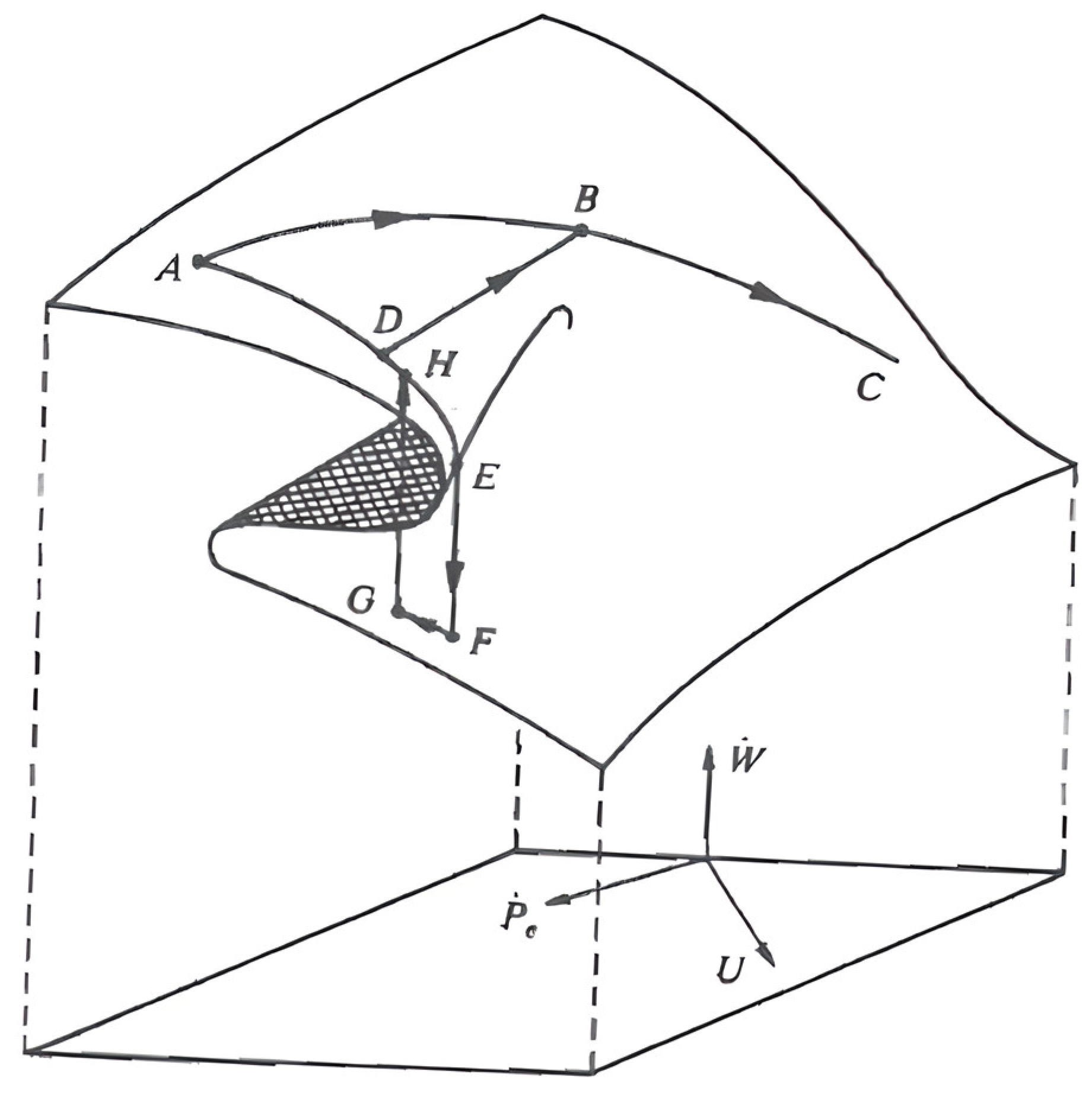
as a state variable, although in this last case, the effective rate of price growth could also be used. Taking all this into account, we would have the graphic representation of the “cusp” (
Figure 1) referring to the specific problem that we have chosen as an illustrative example [
19].
The position marked by point indicates a high expectation of price growth. The intention to reduce it would suppose an increase in unemployment, following the trajectory , although there could also be an increase in unemployment without giving up the expectative of inflation, which would mean following the trajectory , that would correspond to the “stagflation” situation. Exiting the zone can occur in two different ways: by choosing the option of a not excessively rapid increase in unemployment while initiating actions that guarantee a clear improvement in expected inflation (path ); or by collapsing the situation through a decrease in inflation in exchange for a drastic growth of unemployment trajectory .
There is also the possibility of contemplating an attempt to reduce unemployment from the last position ( point), even if this means returning to higher levels of inflation. This would suppose a new discontinuity or catastrophe through a trajectory such as the , in which the hysteresis principle or phenomenon is obviously fulfilled. This phase of the process could be assimilated into the concept of the “natural rate of unemployment” of the accelerationist theory of inflation, in the sense that any attempt to reduce the percentage of unemployment below such a one only translates into a constant increase in inflation.
To conclude this section, we want to draw attention to something that could lead to doubts and confusion, and it is the fact that, being the continuity in the deformation process substantial in topology, we can consider that it breaks when the collapse occurs when passing from point to point of the cusp, although it is not. Effectively, if we see the surface as if it were a sheet of paper forming its profile, a kind of capital S, it can be verified that the continuity is not altered, thus complying with the requirement. The abrupt fall of the upper point of the fold of the sheet on the lower surface of the same is considered an alternative path that certainly constitutes a discontinuity, the first of which can be of five properties that, according to Zeeman, has the cuspid catastrophe, and that consists in the fact that minimal variations of the slow variables are followed by sudden jumps in the behaviour of the system. The line that joins the points and would represent, in the economic problem that we have raised, the curve corresponding to the long-term Phillips equation, which, instead of being a third-order parabola, as was found for the crisis period of the 1970s, became, in theory, a vertical line whose abscissa point came to indicate the unemployment rate non-accelerating the inflation.
Let us indicate, finally, that most authors agree that Catastrophe Theory and chaos mathematics can be thought of as two approaches to a general theory of discontinuity dynamics. Both share the concept of bifurcation or unfolding of equilibrium at critical points, as well as the fact that functional relationships are more often nonlinear. The original, and in a certain sense controversial work of the French mathematician undoubtedly supposes an important contribution to the development of differential topology, although it turns out to be a fundamentally programmatic approach if one considers, as Thom himself reminds us, that “là où il n’y a pas de théorème, il n’y a pas de théorie” [
20] (p. 521).
3. The Mathematics of Chaos: A Short Review
Chaos is a ubiquitous universal phenomenon that can be observed in any area of science, from the three bodies of celestial mechanics to Hamiltonians, particle accelerators, fluid dynamics, chemical reactions, biological systems, and the field of economics. Lyapunov exponents help to characterise chaotic behaviour by providing a measure of the local instability of a system in the sense of the exponential separation between two initially neighbouring trajectories:
The limits
or
are both (6) and (7) Lyapunov exponent expressions. In a dynamical system, there will be as many Lyapunov exponents as there are degrees of freedom (number of state variables), representing each exponent as the mean rate of contraction or expansion of the solution of the system in each axis of the phase space. Simple dynamic attractors can be distinguished from complex dynamic attractors by means of these Lyapunov exponents. These attractors are dynamic equilibrium, i.e., a bounded region of phase space in which a system tends to evolve. Simple dynamics attractors are the fixed points, limit cycles and quasi-periodic torus that we could say were the only existing attractors until Lorenz’s contribution in 1963. Complex dynamics attractors are chaotic or strange attractors.
We call simple dynamics fixed points, limit cycles, or tori because, inside these attractors, two nearby orbits starting from arbitrarily close initial conditions always remain close, guaranteeing the accuracy of prediction of the system in the long run. By contrast, in a system with chaotic behaviour, the evolution of any solution should be bounded inside a strange attractor but should also be locally unstable. This implies that the trajectories described by the solution to a chaotic system are irregular and aperiodic, with sensitive dependence on initial conditions. This complex dynamic of strange attractors makes predictions beyond the very short term difficult.
As the Lyapunov exponent can be used to measure local instability, they can be used to distinguish between “simple dynamics” and “complex dynamics”. More concretely, chaos can be detected in dissipative systems when there is a positive Lyapunov exponent. In one-dimension dynamics, the only possible attractors that can exist are fixed points, which the Lyapunov exponent, , should be negative = −). In systems with two dimensions, the attractors could be either fixed points or limit cycles with, = (−) and (, ) = (−, 0) respectively. In three dimensions, one would have:
(, , ) = (−, −, −) ➝ (stable fixed point)
(, , ) = (0, −, −) ➝ (stable limit cycles))
(, , ) = (−, 0, 0) ➝ (stable torus)
(, , ) = (+, 0, −) ➝ (strange attractor)
The strangeness and local instability of chaotic attractors are related to the fact that these attractors are fractals, geometric objects that have a beautiful microscopic structure. This new geometry of complexity was created by Benoît Mandelbrot, who in 1975 published his novel work The Fractal Geometry of Nature. He was educated at “École Normale” and the “École Polytechnique” and with that fractal geometry, he aimed to challenge the uninhibited formality of the Bourbaki group, thereby restoring the image and prestige of Henri Poincaré.
The fractal geometry concerns a new concept of measure and dimension beyond the Euclidian one. Fractals are geometric objects with fractal dimensions; that is, they do not take up all the space corresponding to their Euclidean dimension. The dimension of fractal objects is less than the number of state variables or degrees of freedom of the system, and this means that not all theoretically potential states are exploited. A fractal could be seen as a geometric form that remains unaltered no matter at what scale. One might say that, to a certain extent, the structure of a fractal is the same at every scale. This is the opposite of what happens in the phenomenon of renormalization, in which the figures significantly change when observed at different scales. The size of a fractal is given by its dimension, which is not necessarily an integer. This fractal dimension, originally called the Hausdorff-Besicovitch dimension, provides a numeric measurement of the degree of rigorousness of the fractal, a measure of how this geometric object occupies space. One of the methods used to measure fractals is based on the concept of homothecy in Euclidean geometry. Fractal dimensions can be derived using the concept of capacity:
where
is the minimum number of
n-dimensional
-sided cubes required to cover the subset of the
n-dimensional space
. The implicit definition in (8) implies that for small values of
:
The capacity or dimension of a point, a line, and a plane is 0, 1 and 2, respectively. That is, the number of hypercubes of side
required to cover a point, a line and the surface of a plane would be proportional to 1/
, 1/
, and 1/
respectively. As mentioned above, a fractal is a geometric object whose dimension is strictly greater than its Euclidean capacity. The Cantor set and the Kotch curve, typical examples of fractals, have fractal dimensions greater than 0 and 1, respectively:
In addition to the fractal dimension and the Lyapunov exponent, another key concept in the analysis of complex dynamics is bifurcation. A bifurcation occurs when the period of the orbit is doubled when some system parameter is changed. One can explore the comparative dynamics of a system, that is, the different types of attractors that a model can achieve when the value of a parameter is changed through the analysis of bifurcations. Bifurcation is the way in which the system moves from one attractor to another when a structural parameter changes. Considering the essential contributions of Yorke, May, and Stephen Smale and the decisive work of David Ruelle and Floris Taken in the “Institut des Hautes Études Scientifiques”, perhaps the best illustrative example of comparative dynamics through bifurcation is the Feigenbaum tree [
7] (pp. 5–11). Consider, for example, the logistic map:
where the parameter
determines the type of dynamic equilibrium or attractor of the map:
0 ≤ < 3 → a single stable fixed point
= 3 → the fixed point becomes marginally stable
> 3 → the fixed point turns unstable
= 3.2 → period 2 limit cycle
= 3.5 → period 4 limit cycle
= 3.56 → period 8 limit cycle
= 3.567 → period 16 limit cycle
= 3.58→→→the cascade of duplications accelerates, and the attractor becomes chaotic
The graph of bifurcation, also called the Feigenbaum Tree, is represented in
Figure 2 and shows the bifurcation or duplication of the attractor period of the model as the
a parameter increases. The scale factor of the
parameter for doubling the period of the attractor:
converges towards a constant
= 4.66922, known as the universal Feigenbaum number. An interesting characteristic feature of chaotic systems is that inside the range of values where the map behaves chaotically, there are some windows of periodicity and order. These windows are represented in the bifurcation diagram by clear patches within the shaded zone of chaos, representing periodic limit cycles with an odd period, a property used by Li and York to define chaos [
7] (pp. 5–11).
4. Tests Detecting Chaos in Economic Time Series
Economic theory does not face major conceptual difficulties that prevent it from defining theoretical economic models with chaotic behaviour. In fact, there are many contributions generalizing the traditional economic models to behave chaotically under economically plausible assumptions. On the contrary, there is no robust empirical evidence that detects chaos in observed time series in economics or finance. In this sense, the main focus of the most recent contributions on chaos in economics deals with the development of new tools and techniques to detect chaotic behaviour in economic time series. That is, tools to test whether the underlying economic process is chaotic or, on the contrary, a simple dynamic system with perhaps an added purely random process. Chaos is disorder and determinism at the same time. And, given that economic time series are highly irregular, we want to discern when this disorder has a chaotic origin.
The first step to detect chaotic behaviour in the underlying dynamics generating a time series is to search for evidence of nonlinear dependence. The BDS test and the Hurst exponent are the most widely used tests for time dependence, whether linear or nonlinear. These BDS and Hurst statistics allow the nonlinearity test of a time series if all linear dependence has previously been eliminated, and this can be achieved by obtaining the residuals of a fitted series using an ARMA process.
Having established nonlinear dependence, the next step to test for chaos in a time series involves the estimation of the fractal dimension and the Lyapunov exponent of the attractor of the underlying system. The main restriction we may face is that the attractor of the underlying system is rarely known, so it is difficult to estimate these measures of chaos. For this reason, to estimate the Lyapunov exponents and the fractal dimension from a time series, it is necessary to recover or reconstruct the underlying attractor while ensuring that the qualitative properties of the underlying unknown dynamical system are preserved.
One of the most commonly used methods for reconstructing the underlying attractor is based on the embedding theorem of Takens using lagged time series data. This method allows the reconstruction of an attractor that preserves the topological properties of the original unknown attractor; that is, it is equivalent in its dynamic and geometric properties. We can obtain the relevant information, such as the fractal dimension and Lyapunov exponents of the underlying dynamical system, to detect chaos in a time series, even when the generating systems are unknown.
A fractal dimension is a measure of the attractor that uses alternative metric concepts for length, area or volume. A fractal dimension is estimated using hyper-cube covers of the phase space. The probabilistic fractal dimension, which is more generally used in economics, where time series usually have measurement errors, is the correlation dimension. This method consists, basically, in using hyper-cubes of radius
r to count the frequency at which two points in the phase space are close together as a consequence of the system [
15]. The correlation integral between two points is:
where
is the hyper-sphere radius,
is the embedding dimension, and
is known as the correlation dimension. Taking the logarithm gives us:
and, therefore,
This is the correlation dimension; its values have been demonstrated by Grassberger and Procaccia to be near the capacity dimension but without exceeding them,
[
10] (pp. 189–208).
If the correlation dimensions grow with the embedding dimensions
, the process should be considered stochastic, whereas if correlation dimensions converge to a value independent of
the process will be deterministic. The fractal dimension can be used to measure the complexity of the attractor. However, the estimation of this fractal dimension, by using, for example, the correlation dimension, cannot be considered as a sufficient condition in testing for chaos in a time series. The reason is, among others, that we have to accept that there is always some random component in economic time series, so estimates of the correlation dimension may be biased upwards, confounding the detection of truly low-dimensional chaotic behaviour. Therefore, fractal dimension estimates are usually considered complementary to other techniques for detecting chaos, in particular, the Lyapunov exponent spectrum. Recall that the presence of a positive Lyapunov exponent in dissipative systems indicates a sensitive dependence on initial conditions, that is, chaotic dynamics. In this sense, different contributions have appeared in the literature that try to estimate Lyapunov exponents that are consistent even in the presence of random noise in the time series [
21].
Another method previous to detecting chaos is, as we mentioned above, the Hurst exponent that can be estimated through the analysis R/S, where R and S are the range and the standard deviation of a subsample of size
of the time series, respectively. We can estimate the regression between R/S and
in logs to obtain Hurst’s exponent as the slope
of this regression line. The Hurst exponent provides a measure of correlation,
The interpretation of the Hurst exponent can be summarised as follows:
0 < < 0.50 → < 0 (Pink noise)
= 0.50 → = 0 (White noise)
0.50 < < 1 → > 1 (Black noise)
That is, by estimating the Hurst exponent, we can conclude that the time series may be a white noise with no correlation; an antipersistent or ergodic series, i.e., a pink noise; or a persistent time series, i.e., black noise. The pink and black noise can be described using a Fractional Brownian Motion, and its fractal dimension can be estimated as the inverse of
.
The hydrologist Harold Edwin Hurst studied Nile floods using R/S analysis and concluded that optimum dam sizing, or equilibrium position, could be achieved at around 0.67. Long memory persistent time series are in this approach random biased walk, where the magnitude of the bias depends on the degree to which is above 0.50. Such series are fractals, and the inverse of H is a measure of their fractal dimension.
There are other methods or tests to identify whether a time series is chaotic or evolves randomly. These include the BDS test, already mentioned, and the Kaplan test. The BDS statistic asymptotically follows a normal standard distribution under the null of IID, identical and independent distribution. Nonlinearity and chaos are included within the alternative hypothesis. On the other hand, the Kaplan test was initially formulated as a test for determinism, although it has been adapted as a general test for nonlinearities in a time series. This Kaplan test relies on the continuity properties of the phase space of deterministic systems. If the underlying dynamical system is deterministic, then the images of two nearby points will also be close together. On the other hand, if the system is stochastic, the evolution of two initially nearby points should be far apart in the phase space. That is, the Kaplan test is concerned with the evolution of the distance between two initially nearby states [
22] (pp. 469–482).
5. Chaos Topology in Economics
In the ambitious, knowledge-devouring, and multifaceted world of the great French mathematician and physicist Henri Poincaré, there is, without a doubt, a place for topology. Indeed, the restless and tireless scientist who had studied the three-body problem, celestial mechanics, the qualitative theory of differential equations, the theory of Diophantine equations, the theory of numbers, and the theory of special relativity could not ignore the growing importance of algebraic topology, which he would deal with in his well-known “Analysis Situs”.
Although Poincaré’s contribution to topology comes from very different sources and pathways, we can provide a rough idea of what it entailed considering his valuable and controversial conjecture, on the one hand, and the no less discussed problem of the three bodies, on the other. Regarding the conjecture, let us remember the notion of surface understood as a geometric figure that can be obtained by deforming, curving, and conveniently joining one or several pieces of the plane. The way in which these deformations are carried out leads to diverse types of surfaces, each with different properties, being able to cite, as examples, the cylinders, the spheres, the ellipsoids, and the paraboloids or tori. Regarding the three-body problem, we have already referred to it previously, highlighting the fundamental issues. In any case, we remind the reader that in Chapter II, Volume I of his book “Les méthodes Nouvelles de la mécanique celeste” [
23], Poincaré, basing himself on Jacobi’s 1st and 2nd theorems and the use of Keplerian variables, explains with an extremely formalized rigorous approach the three-body problem.
In a clear and direct way, we must say that in addition to defining the essential content of chaos theory and using various tests to find out if a time series is random or if it is of the deterministic chaotic type, chaos mathematics has a specific content broader and more complete in which topology or qualitative geometry is not absent. As we already have said, Poincaré’s development of topology included new creative ways to study the properties of differential equations. Gilmore, Letellier, and Lefranc affirm that… “ideas and tools from this branch of mathematics are particularly well suited to describe and to classify a restricted but enormously rich class of chaotic dynamical systems, and thus the term chaos topology refers to the description of such systems” [
24]. The usefulness of these chaotic systems lies in the fact that they are embedded in a three-dimensional space, making them easy to visualise.
Physics and economics are the two fields of science where topology plays a role of special relevance, which are also of great importance in their contribution to the development and applications of chaos theory. Because of this, it is necessary to have in mind the content, characteristics, and possibilities of topology. In economics, as an example, we can remember that in a bright contribution, von Neumann uses a topological proposition, the Brouwer fixed point theorem, which can prove that his general equilibrium model has a solution. This constitutes a good proof of the great importance of analyzing the meaning of topology in the framework of economic theory. The problem of the three bodies, for its part, as can be deduced from what we have exposed at the time, is without a doubt another example of the role that topology can play, this time in the field of mathematics applied to astrophysics.
Beyond metric and projective geometry, respectively inspired by the notions of distance and straight line, appears the “qualitative”, the topology, a third geometry in which quantity does not work. In topology, two shapes are always equivalent to each other when one can be transformed from one to the other by means of a continuous deformation. For example, when we apply pressure to deform a rubber band without breaking it, some properties, such as length, will change, but others, the topological properties, will remain unchanged. Topology has allowed the development of the theory of dimension, Poincaré’s polygon, the differential geometry of curves and surfaces, etc. [
7] (pp. 83–84).
For the purposes of expanding what we have said about topology, let us point out that this peculiar branch of geometry can be subdivided into combinatorial and set topology, on the one hand, and in general, algebraic and differential topology, on the other. But frequently, as a third option, a distinction is made between knot theory and manifold theory, the latter being considered by most topologists as the central point of their discipline. To avoid a complex and excessively formalized exposition, we are going to go ahead and summarize our considerations on the nature and content of topology, addressing some issues and problems raised, studied, and resolved by two great figures who dealt with the matter. We are referring to Leonhard Euler, on the one hand, and Henri Poincaré, on the other, the first initiator and the second great protagonist and referent, as we know. Swiss mathematician and physicist Leonhard Euler found the solution in 1736 to the well-known problem of the Königsberg bridges, a solution considered the first theorem of graph theory. Years later, in 1750, he published what is known as Euler’s polyhedral theorem, which consists of looking for a relationship between the number of faces, edges and vertices in the polyhedral, and which can be expressed very simply as follows. If
,
and
respectively denote the numbers of vertices, edges, and faces for any regular polyhedral, it is always true that
or the number of faces (
) plus the number of vertices (
) equals the number of edges (
) plus 2, which is the same.
This formula also applies to any simple irregular polyhedron, i.e., it has no holes, so its surface can be continuously deformed into that of a sphere. Euler’s formula is then extended in the form
for polyhedral with
holes, considering that a simple polyhedron is one which
= 0.
It is necessary to highlight that the number
−
+
, called the Euler characteristic number, will have the same value for all maps of our surface, and the number
is called the genus of the surface. The relationship between two numbers in (16) obviously remains invariant when the surface is continuously deformed. Intrinsic geometric properties of this type, which have little relation to lengths, areas, and volumes, are called topological, and their study has offered and continues to offer very variable perspectives to different fields of mathematics and important branches of science [
7].
We have already commented at the beginning of this section on the fundamental role played by Henri Poincaré in the development of algebraic topology and, within his vast field of research, the close relationship with the birth of chaos theory. On this, as we have done with Leonhard Euler, we want to go deeper, within the limitations that we have imposed ourselves, around the very personal contribution made by the great French mathematician in this matter. Let us remember that Poincaré was the progenitor of what we now call chaos. He described it as follows: “It may happen that small differences in the initial conditions produce very great ones in the final phenomena. A small error in the former will produce an enormous in the latter” [
25] (p. 48), [
14] (pp. 21–22). It is interesting to remember that his Analysis Situs, already mentioned, is reached by his attempts at qualitative integration of the differential equations. The Poincaré geometric intuitionist approach, which contrasts with Hilbert’s formalist, serves as the basis for some of the approaches to chaos mathematics, which owes not a little to the seminal work of the prestigious, restless, and versatile French mathematician.
To better understand the topological component in the theory of chaos, it seems advisable to establish the connection between two elements, notions, or fundamental instruments of the same: the attractor and fractal concepts, which we have briefly discussed above. Do not forget, as we have said in the corresponding section, that the relationship of transformation and equivalence existing between them is clearly topological; in other words, it is of a qualitative geometry. First, let us point out that the trajectories shown in the Lorenz and Rössler attractors, for instance, are solutions of two respective first-order nonlinear ordinary differential equations, being the motion described by them being deterministic, bounded, and recurrent.
It is important to know that the essential geometrics of chaos consist of stretching and bending, as pointed out by Stephen Smale in his topologic transformations. In effect, the irregularity of movement is produced by a mechanism that is broken down into two actions. On the one hand, the spatial phase is stretched by separating trajectories, and then it doubles back into itself, or what is the same, we have a process of stretching and squeezing. Stretching is responsible for sensitivity to initial conditions that can be quantitatively measured using positive Lyapunov exponents. Squeezing is measured using the negative Lyapunov exponents, which in turn is responsible for building up a layered structure, like a millefeuille, that provides the fractal structure to strange attractors [
24].
The construction of an attractor, such as Rössler, is performed by the repetition of stretching and folding. The folded parts of the attractor are squeezed together to build up a fractal. This process, of topological nature, allows us to affirm that chaotic attractors are fractals, geometric objects that have a beautiful microscopic structure developed within the framework of a new form of the geometry of nature or complexity, a framework created by Benoît Mandelbrot, who in 1975 published his famous work “The Fractal Geometry of Nature”.
It should be noted that the analysis of chaotic dissipative systems in the chaotic regime has led to the advance of new topological methods that, although originally developed for three-dimensional systems, are also applicable to any “low-dimensional” system, which can be reflected in a three-dimensional subspace of phase space. Logically, the associated attractor should have Lyapunov dimension
< 3. These topological methods supplement those metric and dynamical invariants previously stated. As pointed out by R. Gilmore…: “topological methods possess three additional features: they describe how to model the dynamics; they allow validation of the models so developed; and the topological invariants are robust under changes in control-parameter values” [
26] (pp. 1460–1461).
The main objective of the analysis of dynamical systems under the topology approach is the identification of the stretching and squeezing forces driving the aperiodic orbits of the systems inside strange attractors. These mechanisms stretching and squeezing the phase space are represented by a branched manifold called a template or a knot holder, terms and concepts to which we have already referred above.
Before concluding this section and thinking about the role of topology in advancing chaos theory and its applications, we would like to mention professor Dennis Sullivan for the wide perspectives he opens with his books and articles on the subject. As culmination of his fruitful career, the prestigious mathematician has won the 2022 Abel Prize “for his contribution to topology in its broadest sense and in particular in its algebraic, geometry and dynamical aspects, introducing new concepts, proving landmark theorems, answering old conjectures and formulating news problems that have driven the fields forwards”. The extensive area of study and research undertaken by the great American mathematician has led to being frequently called or known as the “Unifier of Topology and Chaos”.
6. Computing and Chaos
Following previous renowned authors, we have already had the opportunity to say in other contributions that the quantum theory, the theory of relativity, and chaos theory are the three winning discoveries of the 20th century [
7]. However, there is a fundamental difference between the two great conquests of science, relativity and quantum physics, on the one hand, and chaos theory, on the other. The first two are great, decisive, and consolidated branches or fields of science. What we call chaos theory, on the other hand, is a set of techniques and mathematical tools conceived as an instrument, or logical support, for those sciences in which complexity is an irrefutable fact, where nonlinearity constitutes a characteristic of a dynamic system, and where there is an important dependence on small variations in the initial conditions. Does this mean that we should neither use the expression chaos theory nor have it act at the same level as the theory of relativity and quantum theory? Within a strict and rigorous criterion, the answer would be yes since comparisons cannot be made when there is no homogeneity. But this in no way diminishes the wide range of applications of the mathematics of chaos techniques and the important successes and advances achieved in a relatively short period of time [
7] (pp. 75–78).
It is often said that where there is chaos, there is no possibility of prediction. This is a wrong identification of chaos with randomness, inconsistent with the very definition of chaotic behaviour, as under the disguise of irregularity hides a deterministic law that we must discover. Chaos does not always imply low predictability. An orbit can be effectively chaotic and still be predictable in the sense that it is followed or shadowed by a real orbit. This makes its prediction physically valid.
Chaos theory has made a decisive contribution to solving many problems that we found intractable in the past [
7,
27,
28]. Among them and considering the applications in different scientific fields, we can mention, by way of example, cardiological and neurophysiological episodes, sequencing of the human genome, complex studies on atmospheric phenomena, policy analysis, decision making, capital markets evolution, or the novel problem of the management and control of certain chaotic processes in response to their potential consequences. Of course, there is still a huge research effort ahead.
Reflecting on the matter, the famous British mathematician Roger Penrose, to whom we shall return later in another section, states “that despite such profound difficulties for deterministic prediction, all the normal systems that are referred to as chaotic are to be included in what I call computational. Why is this?” [
29] (p. 23). Penrose himself answers that to decide that a procedure is computational, we must know whether it can be put into an ordinary computer. On this basis, we allow ourselves to add that we can include chaotic systems since he works with long, apparently random series but with great frequency, and after applying the various tests, they are deterministic series that hide important laws and behaviours.
Given the above, a fundamental question remains regarding the usefulness of establishing a profitable relationship between chaos and computing. Penrose, to whom we have already referred, gave a detailed analysis of the matter in his enchanting book on the Shadows of the Mind written, as we know, in 1994, concluding that “chaos does not really get us out of our difficulties with the computational model” [
29] (p. 179). However, in recent years, some books and papers have been published in which we find new approaches relating to the possibilities of Chaos Computing. In this regard, as professor Miguel A.F. Sanjuan affirmed in a recent work, “Machine learning and deep learning techniques are contributing much to the advancement of science. Their powerful predictive capabilities appear in numerous disciplines, including chaotic dynamics, but they miss understanding” [
30] (pp. 1–5). According to professor Sanjuan, in research from the University of Maryland, veteran chaos theorist Edward Ott and their collaborators have employed a “machine-learning” algorithm called “reservoir computing” to understand the dynamics of an archetypal chaotic system, the Kuramoto-Sivashinsky equation, consisting of the important result in the fact that after training the equation with past data, they were able to predict the evolution of the system out to eight Lyapunov times into the future, what basically means eight times further ahead than the previous methods allowed. Integrating the machine learning approach and traditional model-based prediction could obtain accurate predictions twelve Lyapunov times.
It is convenient to clarify before going on that the term “reservoir” refers to the internal structure of the computer and that it must meet two requirements, or if you prefer, that it is characterized by two properties. Firstly, it must consist of nonlinear individual units, and secondly, it may be able to store information. The nonlinear response of each unit to input allows reservoir computers to solve complex problems. Reservoirs can store information by linking the units in recurrent loops, where the previous input influences the next response. The computers learn specific tasks by training and using information about past interactions.
In this connection, it should be emphasised that the work and research on computing and chaos must benefit all technological advances and, at the same time, make full use of the valuable tools and methods of Statistical Science. In this line, Escot and Sandubete make use of new computing techniques to estimate the Lyapunov exponents, which, as seen in the previous sections, is one of the main indicators of the existence of chaotic behaviour behind a time series [
21]. The authors have illustrated the robustness of the algorithms proposed for estimating the Lyapunov exponent from several noise-contaminated time series, comparing the results provided by the traditional direct methods with those of the Jacobian indirect ones and demonstrating that the indirect methods provide better estimates than direct methods in all the experiments that they have conducted. Achievements of this type are the ones that really matter, beyond more or less clear and debatable considerations about the scope and possibilities of Q.A.I. and its impact, among other areas, on chaos theory itself.
As the authors say, this method or approach “could motivate the scientific community in this area where new contributions may appear considering new machine learning methods and statistical procedures to obtain robust Lyapunov exponent estimators on a noisy environment in which the presence of just a (small) measurement noise can lead to confusion between a chaotic deterministic system and a purely stochastic one” [
21].
Once the existence of chaotic behaviour has been detected through the estimation of Lyapunov exponents, the machine learning algorithms can also help improve the predictions of these chaotic time series. Ramadevi and Bingi present a review of significant contributions on various approaches using machine learning techniques for chaotic time series forecasting, such as convolutional neural network (CNN), wavelet neural network (WNN), fuzzy neural network (FNN), and long short-term memory (LSTM) in the nonlinear system. These predictive models have demonstrated greater accuracy and better results than traditional statistical models [
31].
7. On Current and Future Research and Applications to Economics
The evolution of chaos theory and its applications has experienced ups and downs and known moments of boom and bust. This has indeed happened with economics, which, together with physics, constitute the branches of science that, from their beginnings, stood out in this important field of knowledge.
In our book published in 2019 with the title “Chaos Theory: Current and Future Research and Applications” [
7], in a concise note on the history of chaos, we distinguished five phases or stages: The birth of chaos, highlighting the Poincaré phase space; the definitive birth, with the unexpected discovery of meteorologist Lorenz; the golden age, in which it was given an intensive use of mathematics and techniques of chaos; a brief stage of relative slowdown, and finally, new research and applications by way of “renaissance” [
7] (pp. 23–27).
If we stick to the last three stages, we can have a clear vision of the subject-object of our analysis. The third one, sometimes known as the “golden age”, covers part of the eighties, the whole of the nineties and the beginning of the 21st century. The use of what we could call the techniques and mathematics of chaos has intensified, incorporating other contributions from outstanding researchers into this recent branch of science. Over this broad period, as we saw in
Section 3 of our work, we find ourselves with Feigenbaum’s bifurcation diagrams, the Mandelbrot fractal geometry of nature, Grassberger and Procaccia’s work on the characterization of strange attractors, the contribution of McCauley on chaos, dynamics and fractal, and the very well-known book written by Alligood, Sauer and Yorke.
But it is necessary to point out that what we have called the golden age was progressively fading, giving way to a brief stage of relative slowdown in the development of chaos theory, perhaps due to studies being limited to insisting on the principles and bases of the new theory but, with a few exceptions such as the work edited in 1992 by J.H. Kim and J. Stringer, without going into the important and necessary chapter on applications in different scientific fields. We must highlight that at a time when chaos theory accentuated its presence and importance, the deep understanding and close relationship between physics and economics gave rise to the fact that both fields of science stood out in research and studies on the subject, as can be verified by analysing the literature on the subject. However, the concentration of knowledge in these two branches had scant attention directed towards other areas of science, although this situation would change after this brief parenthesis. Effectively, from the middle of the first decade of the 21st century to the present, there has been a veritable avalanche of research and applications in such important sciences as biology and medicine, as well as in the field of engineering in its different specialities.
Some of these scientific branches are studied together, giving rise to a new type of application. For instance, there is a new line of research named “synthetic biology” that integrates different scientific areas, such as nonlinear dynamics, the physics of complex systems, engineering, and molecular biology. The emergent field of research is intrinsically interdisciplinary and constitutes an advance to consider over the coming years in our work on the application of chaos and complexity theories. The studies of complex networks in physics, mathematics, economics, and other sciences are also presently undergoing a very important development, which represents new possibilities in the task that we are undertaking.
Undoubtedly, the achievements in the field of physics and economics through a profusion of books and articles are serving as a guide for the application of chaos in the other sciences that we have mentioned, which, in a feedback process, can provide new ideas and trends that result in a new awakening of the pioneering branches in the study of chaos, that is, in in the physics–economics binomial. From all this, and given the great advances in computing, it can be deduced that both physics and economics are faced with new possibilities to deepen the content and development of chaos theory and its applications.
If we stop at the specific case of economics, which is what really interests us now, we are presented with a promising but, at the same time, complicated panorama. First of all, it is necessary to point out that many books and articles that deal with the applications of chaos theory in economics focus on the analysis of capital markets, which is due to the fact that this subject, in addition to its importance, contains long series that allow reliable and empirically well-founded studies. But we can also say that there are several important branches of economics, among which the following deserve mention: economic growth, cycles, income distribution, general equilibrium, inflation, unemployment, demand regulation, economic development, and foreign exchange rates.
In 2013, professors Fernández Díaz, A. and Grau-Carles, P., published the third edition of the book “Chaotic Dynamics in Economics: Theory and applications”. In it, and after addressing the deterministic chaos, the inevitable complexity, the nonlinear dynamics and the mathematics and techniques of chaos, on the one hand, and the applications to the different- areas of the economy, on the other, the authors carry out an exhaustive empirical analysis in which the financial–economic crisis of the period 2006–2013 is treated.
This was a period characterised by strong oscillations and high volatility in the markets, especially since the stock market hysteria on Monday, 21 January 2008, resulted from the fear of a recession in the United States economy following the start of the enormous mortgage fraud. We apply the techniques described in the previous sections to analyse the dynamics of the Spanish stock market in search of chaotic behaviour. The analysis was realized with the time series of IBEX 35 daily data during the referred period, studying the time evolution of IBEX daily returns obtained as the composed returns or the first difference of logarithm of stock prices (
Figure 3).
The statistical summary of the data is shown in
Table 1. The mean daily return is close to 0, while the daily volatility is around 1.7%. The smallest daily return is −9.6%, and the largest is 13.4%. The distribution of daily returns shows a positive and small asymmetry and a high kurtosis. The Jarque–Bera test rejects the hypothesis of normality, and the Ljung–Box test is involved with the presence of autocorrelation.
Applying the chaos detection tests and taking into account all the results obtained in our empirical analysis, we cannot clearly conclude that the IBEX 35 daily returns in the period 2006–2013 are covered by a chaotic deterministic system. The series could also correspond to a nonlinear dynamical system with noise far from equilibrium, subject to bifurcations or changes in its dynamics. In an attempt to understand the reasons for this behaviour, we can state that the irregularities and disequilibrium in the economy and the international financial markets can be explained by ethical, political, and institutional factors during the period analysed. Key elements in explaining the unusual and unconventional functioning of the capital markets in the years of the crisis are the existence of corruption in the behaviour of rating agencies with oligopolistic power in the scoring of financial assets and colluding with groups of brokers. All this can be interpreted as evidence that there has been something more hazardous or that there has been a chaotic behaviour in the evolution of the series of values, as has been seen, with some ability to predict. For a review of the main contributions to detecting chaos in financial time series, see the article by Faggini, Bruno, and Parziale, which also shows a systematized table summarizing modern methods to detect chaos that provides a quick reference of the current state of research in this field [
32] (p. 21).
Chaos theory also has important applications to the real economy, such as the study of economic crises, inflation, and monetary policies, so relevant in a situation like the current one. Chaos theory allows the explanation of situations of economic instability, inflation and unemployment in an endogenous way, providing an alternative approach to the well-known real business cycle models in which the business cycle and economic instability are explained by the existence of purely exogenous shocks. Chaos application to the real economy requires the introduction of nonlinearities in the modelling of economic performance, with, for example, nonlinear Phillips curves, production functions with nonlinear restrictions, or nonlinear income distribution rules [
7].
In this sense, chaos theory not only provides a new explanation for economic instability but also furnishes the tools to control such instability. The control chaos techniques allow the economy to be stabilized with automatic and not-too-invasive economic policy rules (they do not require a major structural change in the models). These rules of chaos control have been applied, for example, to the analysis of monetary policy as an instrument to achieve price stability [
33]. Rules, which are optimally derived by applying chaos control, have also turned out to be very similar to the now widely known Taylor rules of monetary policy, in which the instruments of monetary control are applied in response to deviations of inflation and unemployment from their target values. All these applications of chaos theory to economic policy recover the discussions about the differences in discretional and automatic stabilizers in economic policy, thus contributing to an advance with respect to such a relevant subject [
19].
With the new instruments, capabilities and algorithms that we have considered in the previous section (computing and chaos), the use of time series will undoubtedly be significantly faster and more effective. Something similar could be said of other branches of economics, although it is not appropriate to enter them given the structure of our work, being able to conclude that the application of chaos to economics, counting on the recent advances, seems to enjoy stimulating perspectives.
8. Coda
“When I came to consider a little more closely the nature and mode of human knowledge, I found that there was much to deal with in regard to propositions, and that words, either from custom or necessity, were so mixed up with knowledge, that was impossible to discuss it as clearly as one wanted without first saying something of words and language”.
John Locke: “An Essay Concerning Human Understanding”, Book III. Of Words. (1689/90).
As a brief conclusion, and independently of the message derived from the musical illustration that closes these lines, we are going to remember the fundamental questions that have been addressed in this article on chaos theory and its applications to economics, presented as a current vision and with a short-term future.
First of all, we must remember that we have highlighted the terms and concepts related to nonlinearity, dynamical systems, dependence on initial conditions, complexity, fractals, attractors and their different dimensions, strange attractors, fractal dimensions, bifurcations, tests for detecting chaos, and so on.
Since our approach looks more to the future than to the past, and considering that it is written for a mathematics review, we have dedicated separate sections referring to the use of Catastrophe Theory, chaos topology, computing and chaos, machine learning algorithms (Reservoir computing), and statistical procedures to obtain robust Lyapunov exponent estimators on a noisy environment, something very important to avoid confusion between deterministic chaos and stochastic one. We place most of these more advanced techniques within the framework of Artificial Intelligence, at least in the part of it that is already consolidated.
Responding to the title of the article, we have referred the applications of chaos theory to their various areas and the main problems of the economy, to nature, and to the financial sector. Regarding the real economy, we consider the application to the stagflation problem, the Keynesian demand, the monetary demand, the general equilibrium, Cycles and Growth, the income distribution, the exchange rates returns and volatility, etc., sending the reader to the corresponding references. Regarding financial economics, and given that in it, we can handle very long series, the behaviour of the Madrid Stock Exchange during the 2006–2013 period is addressed in a specific way. With the application of the different chaos tests, we can find out if the Madrid stock market behaved as a random phenomenon or, in contrast, if it functioned in a deterministic way that distorted stock market evolution. In other words, the empirical case shows the way to determine if an event is due to pure hazard or if, behind an apparent disorder, there is a law that, in a deterministic manner, would demonstrate the causes of said behaviour and the existence of chaos.
![Mathematics 12 00092 i001]()


