1. Introduction
The Paris Agreement has created significant awareness of challenges related to climate change and has formally been adopted by 196 parties [
1], whereby they are required to develop and implement plans for climate change action through Nationally Determined Contributions (NDCs) to advance in the direction of the goals of the agreement [
2,
3]. The primary goal of these NDCs is to reduce carbon dioxide (CO
2) and other greenhouse gas (GHG) emissions [
4]. It has been estimated that to achieve the Paris Agreement goals, deeper decarbonization efforts are needed, such as working towards 100% renewable energy systems.
The transportation sector, which primarily relies on oil as a fuel, is one of the most challenging sectors to fully decarbonize [
5,
6], and its overall response to the newer climate policies has been slow [
7,
8]. Additionally, the transportation sector is among the main contributors to global CO
2 emissions, accounting for around 16.2% of global CO
2 emissions by 2020 [
9]. In this context, the electrification of the transport sector (electromobility) will lead to an important reduction in its carbon footprint. Electric Vehicles (EVs) will not only play a major role in reversing the current trend of increasing emissions but also could help increase the flexibility of the energy system [
10]. However, the driving range, cost differentials, and charging infrastructure requirements remain some of the biggest hurdles to overcome in spurring the deployment of EVs [
11]. Indeed, as sales of EVs grow (14% of market share in 2022 [
12]), the EV charging infrastructure becomes more stringent and a significant barrier [
13]. Hence, the literature has analyzed the challenges that electromobility generates regarding the infrastructure associated with charging points and the increase in electrical demand, particularly if that new demand is not well managed [
14,
15]. The authors in [
16] present a critical review of the effects of unmanaged EV charging and examine the benefits of smart charging and Vehicle-to-Grid (V2G) technology. It was found that unmanaged charging increases peak load, leading to high energy losses, voltage violations, voltage imbalance, transformer lifespan reduction, and harmonic distortion. The authors also show that such negative EV impacts are indeed increased if infrastructure planning (EV charging facilities) are not well designed and located. This complexity is exacerbated by compatibility issues related to the available EV charging types, whether the vehicle supports the available charging type, the waiting times in queues, and the charging time [
13,
17,
18]. The technical and regulatory challenges and availability issues can create range anxiety for EV owners, dissuading them from switching to EVs for long-distance travel [
19,
20,
21]. Hence, a coordinated strategy of EV demand response as well as infrastructure planning is required to uplift the benefits that electromobility brings to the decarbonization of the transportation sector.
An alternative option to charging infrastructure planning relates to portable EV chargers and power boosts (power banks on wheels,
Figure 1). Both options represent a simple and space-effective alternative that neither requires infrastructure nor a specific location to be used. For example, an EV driver can simply use it at a parking lot or by the curbside to recharge their EVs, and that would give sufficient power for the EV to carry on its journey or go to the nearest charge point access [
22]. The UFO LetGo Power Station (which can fast charge batteries to 80% within an hour), ZipCharge Go, ZPN Energy’s ZAPME, Blink, Freewire’s Mobi, and Sparkcharge Roadie are some of the already commercially available portable power boosts. However, this technology can still be expensive for customers to purchase or inconvenient for those who cannot afford extra space in their EV to carry a charger all the time. Therefore, EV drivers who may be stranded and without access to a charge point access or a power boost may find it advantageous to opt for a service where, when needed, they can readily request to have a charging service (using a power boost) delivered to them. The list may also include drivers who may opt for such a service, as they may be unwilling to drive to a nearby charge point access due to high congestion at the charging locations or incompatibility of the available charge points.
Trucks or bikes would constitute a traditional transport mode to bring the power bank to the EV, once the request has been made. The charging takes place at the specific parking lot, and once completed, the service vehicle may carry the power bank back to the charging station or go to the next vehicle that has requested service. Another cheaper, cleaner, and faster option for the service vehicle is the usage of drones. Initially used for military, disaster management, aerial imaging, and surveillance purposes, today, the use of a drone extends beyond the sphere of military and defense, and we have seen drone usage in wildlife protection, oilfield detection, and last-mile deliveries for retail, medical supplies, big shipments, and fast food [
23]. Due to the myriad application areas that require specific capabilities that drones can offer, we see drones of different types (fixed wing, multi-rotor, and hybrid) [
24], sizes [
24], capacities (with payload capacities ranging from a few pounds to 1000+ kilogram heavy-duty ones) [
24,
25], autonomy (ranges of few miles to 400+ miles) [
26,
27], multi-drop capabilities [
28,
29], and using different modes of dispatch (tether, chute, drop or dock) [
30]. Additionally, using drones as a service vehicle has advantages: emissions from operating drones are the least among newer technologies (even compared to EVs), it is a cheap and fast form of transporting items, it is not subject to uncertainties in road and traffic conditions (congestion, floods, forest fires, avalanches, etc.), and it can reach remote or inaccessible locations [
31].
Problems addressing the EV charging policy is a prevalent research area, especially in the context of last-mile delivery logistics. In a seminal paper by [
32], the authors consider a problem where a fleet of vehicles with limited range (not necessarily EVs) is assigned to meet customer demands within a time window and can be charged at the customer locations. Using EVs as a delivery vehicle for the same problem is looked at by [
33], with their charge times being proportional to the amount of charge needed until full. The full charge policy is relaxed in [
34,
35,
36] to allow partial recharges. Some authors [
37,
38,
39] allow the charging to be performed at a charging station. In addition, authors have also studied the sizing (PV and BESS) and operational strategies of parking or charging (fast-charging) stations using meta-heuristics [
40,
41]. Approximations of nonlinear charging function are explored in [
42,
43,
44]. Other extensions that authors have looked at involve using a heterogeneous multi-modal delivery vehicle fleet [
45,
46,
47,
48], battery swap stations [
49,
50,
51,
52,
53] or battery-swapping vans [
19,
54,
55]. The recently published articles that look to extend this problem include properties like simultaneous pickup and delivery [
56,
57,
58], considering uncertain demands [
59], and considering parcel lockers as an alternate delivery method [
60].
The consideration of EV–drone pairs in the context of delivery problems is a recent research area. The authors in [
61] introduce the EV Routing Problem with Drones (EVRPD), which is a 2-echelon routing problem, where the EV acts as the moving hub for the drone launch and recovery (which happens at the same location). The EV itself is not allowed to make deliveries. The authors in [
62,
63] allow deliveries to be made by both vehicles, whereas the authors in [
64] consider non-linear EV and drone energy consumption, while also allowing the drone to make multi-drops.
While all of the previous articles try to address the issues of the limited range and charging policies of an EV in some form or the other, there is a lack of literature that addresses these issues beyond the context of last-mile delivery and for individual EV drivers. Furthermore, flipping the role of a drone to act as a service vehicle (rather than a last-mile delivery vehicle) allows faster service and one that can cater to the flexible charging needs of an individual EV without the need for setting up a complex infrastructure, in comparison to deploying battery-swapping vans or vans with built-in charging ports.
Towards this end, we propose two problems to find the optimal scheduling and assignment of service vehicles (drones) to minimize the total waiting time of EV customers. We call them the Power on the go: Single-drop and Double-drop problems. In the first problem, the assumption is that the power bank is capable of charging only one EV at a time before requiring replacement. So, after every EV recharge, the drone must return to the charge point access (CPA) to swap the power bank before it can serve the next EV. The second problem relaxes this assumption and assumes the bank has sufficient energy to serve two consecutive EVs before requiring replacement. The drone can carry the bank to serve two EVs consecutively whenever the drone has sufficient endurance to make the trip from the CPA to the first EV, then to the next EV, and finally back to the CPA. The overall objective of the problem will be to cater to all customers and their needs and minimize their waiting time between requests for service and the start of charging.
We end this section by highlighting the objectives. In the following section, we describe the problem and its assumptions.
Section 3 presents the
Mixed-Integer Linear Program (MILP) model and two heuristic formulations for the problems.
Section 4,
Section 5 and
Section 6 respectively describe the generation of instances, the experimental results and analysis, and conclude with the managerial implications and extension to the problem presented in this article.
Objectives
The research we present in this article has the following objectives:
Define the two charging problems (single and double drops), where the service vehicle (drone) has a specified range. MILP formulations are presented, and the objective of both formulations is to minimize the cumulative wait times between the request and the start of the charging for an EV.
Develop a couple of heuristics (based on order-first split-second scheme) for both problems that achieve a balance between solution quality and runtime.
Explore the time savings of having battery banks capable of serving more than one EV before requiring replacement.
2. Description of the Problem
Our proposed problem addresses the requirement for charging an EV that has (or almost) run out of power. The service request is made by the driver through an app, and the charging takes place at a convenient location (like a parking lot) without the driver having to visit a nearby charging station. Charging occurs through the use of power banks, and for each type of EV, the time to charge may vary. Service vehicles like drones are responsible for transporting the power banks to the charging location. Charging stations (also referred to as charge point access or CPA) act as the base from which the drones can be launched and retrieved. Power bank swapping and drone battery swapping and recharging are carried out at these CPAs.
Each CPA is equipped with a specific number of drones, and each drone has a defined autonomy (in terms of either flight time or flight distance). While assigning an EV to a drone, the autonomy of the drone needs to be considered to determine if it is feasible.
The location of the CPAs and parking lots are known, and a service request can be made before the EV arrives at the specified parking lot. At the earliest, a drone, if assigned to a customer, could leave the CPA as soon as the request is made (in case the drone is idle at the CPA). If a drone is assigned to a new customer while still charging the previous EV, it must finish the current charging, and only after that can it travel to the new customer. As soon as the charging is complete, the drone is expected to return to its dedicated CPA if there are no other customer assignments at that time. This would ensure that once charging is complete and the EV departs, the drone or the power bank is not left unattended in the open parking lot while waiting for the next order (which may not happen).
In theory, this problem allows the expansion of the coverage area of a charge point access through the usage of operational drones. This would ensure that the availability and charging compatibility needs of the customers requesting charging service are met at the earliest possible time. After serving an EV at the specific parking lots, the drone then either returns to the CPA (single drop) or can serve another EV at the same or a different parking lot (double drop), if the autonomy and residual power in the power bank permit so. Toward this end, in the following subsections, we propose two problems based on the number of EVs a single power bank can serve before it requires replacement.
2.1. Power on the Go: Single-Drop Problem
The initial problem is the simplest one, where a drone is capable of making a single charge after and before returning to its assigned CPA. We will call this problem “Power on the Go: Single-Drop problem” (POTG-SD). It is assumed that all CPAs are equipped with one or more drones, and once charging is complete, every drone must return to the CPA, even if another EV gets assigned to it before it reaches the CPA. Once the drone reaches the CPA, a new power bank is picked up, and then the drone leaves for the next customer. If there are no new requests, the drone will sit idle at the CPA until the next customer requesting service is assigned to it. Since it is a single-drop problem, the assumption is that all EVs request full charging, and after charging an EV, there is no sufficient charge left in the power bank to charge another EV.
Figure 2a shows an example of the POTG-SD problem with two CPAs (CPA1 and CPA2), each equipped with two drones. There are three parking lots (PL1, PL2, and PL3) within the range of the drones’ autonomy, and of them, PL2 can be served by both CPA1 and CPA2. As illustrated, every drone can serve only one EV stationed at a parking lot between departing and returning to its respective CPA. So, a service drone from CPA1 can complete a charging trip (represented by the black dashed arrows) like CPA1-PL1-CPA1 or CPA1-PL2-CPA1.
2.2. Power on the Go: Double-Drop Problem
As an extension to the Power on the Go: Single-Drop problem, we have a case where the drone can make two drops, i.e., the power bank is assumed to have sufficient energy to fully charge two EVs before requiring replacement. In this case, if autonomy allows, the drone may leave its CPA, take the power bank to the first location, and charge the EV parked there. Once completed, it flies to the following location (which can be the same parking lot), charges the next assigned EV, and then returns to its respective CPA. We call this problem “Power on the Go: Double-Drop problem” (POTG-DD). The necessary extension arises out of the assumption that a power bank can fully charge two EVs and that all EVs require a full charge at the respective parking lots. Whatever amount may be left after serving the two EVs will not be sufficient to charge another EV fully. So, the drone has to return to the CPA for the replacement of a power bank.
Despite the power bank being capable of charging two EVs, a single drop may happen on occasions where any of the following conditions are met: the autonomy of the drone does not allow a double drop, or when a new EV requests service anytime after charging of the initial vehicle is complete (which would mean the drone has already left the parking lot and is on its way to the CPA or is at the CPA already).
The double-drop problem is inspired by the fact that there are power banks available that can charge two EVs fully. Analyzing the battery capacities of 371 EV brands found on the EV database website (
https://ev-database.org/, accessed on 6 November 2023), the median battery capacity for 80% charge is 56.8 kWh. While there are power banks capable of storing sufficient energy for fully charging a single EV (FreeWire Mobi has a capacity of 80 kWh), there are others (Freewire Boost 200 has 160 kWh capacity) that provide energy that can charge two EVs fully.
Figure 2b shows an example where a drone from CPA2 can serve two EVs in PL3 and PL2, consecutively (represented in red dashed arrows), as the autonomy may allow it, and the power bank deployed is capable of fully charging two EVs before needing replacement.
3. Formulation of the Problems
For both the single-drop and double-drop power-on-the-go problems, the following parameters are assumed: There are N EVs, which arrive (or request service) at a specific parking lot at time . The parking lot allocated to an EV i is . There are a total of D drones, each of them being stationed at a specified CPA, and the CPA assigned to a drone is . Once assigned to an EV stationed at a parking lot, the drone travels to the specific parking lot with the power bank, charges it, and returns to its CPA.
For all the EVs, denotes the time to charge the EV with the power bank being carried by the drone, , . It would depend on the type of bank the drone is carrying, the charging time of the EV based on its spec, and the power requirement defined by the EV driver who had requested the service. Moreover, for a drone i, will denote its autonomy in terms of distance units.
The distances and times to travel in a drone and are also assumed to be known, specifically for that of any CPA and parking lot, i.e., and are known , . Any setup or wait times at the CPA while power bank swapping or pre- and post-charging of the EV are assumed negligible and not considered in the model, although they could be included without compromising the complexity of the formulation.
The objective is to minimize the cumulative wait times between the arrival (service request) and the start of charging for all EVs that are served.
3.1. MILP Formulation for the POTG: Single-Drop Problem
This formulation is based on a Capacitated Vehicle Routing Problem (CVRP) and considers only one set of binary variables. Although before charging, the drone technically arrives from the CPA, and after charging, it returns to the CPA, as our formulation is based on the VRP, we denote it as leaving and returning only once. The time for revisits to the CPA in between two charging jobs is accounted for while calculating the start time for each charging assignment. The following are the variables considered for this problem:
, which would denote if drone i serves the and EV in succession or not.
denoting the latest time to start charging the EV.
The objective is to minimize all wait times for the EV between the request of service and the start of service, which is given in Equation (
1). The constraints for this formulation are defined in Equations (
2)–(
12).
Note that in these formulations, the sets
and
are used. They refer to the set of
N customers and the set of
drones. In Equation (
2), we ensure that for every
EV,
, there is a
one that immediately precedes it, and is served by a certain drone
i. For every
drone visiting a customer
k for the first time,
j should lie in the set of CPAs. Similarly, in Equation (
3), we ensure that for every
EV,
there is a
one that immediately succeeds it (which can be another EV or a CPA) that is served by drone
i. Equation (
4) balances this out such that if drone
i serves EV
j, there should be a node that precedes it and another that succeeds it, and again, it may be a customer or a CPA. Equations (
5) and (
6) ensure that any drone
i,
, should leave its respective CPA once and return to it once. Although in reality, it may visit the CPA multiple times for swapping batteries, for the formulation, we consider that it should leave and return once with the time between nodes adjusted to represent the time taken to return to the CPA from a parking lot and then head to another where the next EV will be serviced.
Equations (
7)–(
11) are big
M constraints, of which the first two are autonomy related for both
and
customers, the autonomy of the
drone should cover at least the distance for the drone from the CPA of the
drone to the parking lot of the EV being served by it and back to the CPA. The latter three are related to the latest start time for the customer nodes. Equations (
9) and (
10) ensure that the service start time for an EV is greater than or equal to the time of its arrival (service request) and the time taken for the assigned drone to leave its CPA and head to the parking lot, where it meets up with the EV. And in Equation (
11), the latest start time for the
EV should be greater than or equal tothe start time of the preceding
EVs plus the total charging time for that EV by the drone
i plus the time needed for the drone to travel from the
parking lot to the
and then to the
parking lot (assuming negligible wait times in between). Equation (
12) ensures that all start times are positive.
3.2. MILP Formulation for the POTG: Double-Drop Problem
Here, we have three sets of variables, two of which are the same as discussed in the previous section. The third set comprises a binary variable that is used to determine if the drone is arriving from the CPA or another parking lot to serve the current EV. Additionally, we use two sets of auxiliary variables to determine if an EV is eligible for a double drop or not. These are:
, , which would denote if drone i serves the and EVs in succession or not.
denoting the latest time to start charging the EV.
, which would denote if the drone visited the CPA prior to serving EV i (=0) or completed a double drop (flew from the previous parking lot directly) at the parking lot for EV i (=1).
and , are the two sets of auxiliary variables.
The objective remains the same, i.e., to minimize all wait times for the EV between the request of service and the start of service, which is given in Equation (
1). The constraints for this formulation are defined in Equations (
13)–(
33).
Equations (
13)–(
20) are similar to Equations (
2)–(
9). Equations (
13) and (
14) ensure that there is a preceding and a succeeding node to every EV that is assigned to the drone
i, and they may be at the respective CPA of the drone. Equation (
15) is the balancing equation. Equations (
16) and (
17) ensure that every drone
i,
leaves and returns to its respective CPA once. The autonomy constraint is checked for an assignment of drone
i in Equations (
18) and (
19). In Equation (
20), we ensure that the start of servicing the first EV by an
drone corresponds to the time of arrival (request for service) by the EV plus the time it takes for the drone to reach the parking lot from its CPA.
Equations (
21)–(
32) involve the variable
that checks if an EV is served by a drone that is arriving from charging another EV (double drop) or from the CPA. Equation (
21) ensures that the value of
for the EV that is served by a drone
i immediately after leaving the CPA for the first time is assigned a value of 0. Equation (
22) satisfies that if
and
, then
. It means that if both nodes
j and
k are consecutively served by drone
i, and if
j was served by the drone that flew from another parking lot before it, then the drone has to visit the CPA for battery swapping after serving
j and before serving node
k. It would also mean that if
and if
, i.e.,
k was served by the drone flying directly from the parking lot where
j got served, then it would mean that before serving
j, the drone had to perform a battery swap and had to visit the CPA, i.e.,
. Equation (
23) ensures this to be the case.
Equations (
24)–(
29) use the two sets of auxiliary variables. They serve the purpose of making sure that double drop constraints are satisfied, i.e., they can only occur when certain conditions are met. These conditions include (as discussed previously) that for an eligible double drop, the autonomy criteria of the drone have to be met, and secondly, the service request for the next EV that gets assigned to a specific drone must happen before or as soon as the previous charging is carried out. This would ensure that the drone does not fly back to its CPA (as it would be in an idle state as soon as the previous charging is complete and would have to return to the CPA if it does not receive an assignment by then).
Equations (
24)–(
26) use
to ensure that if
= 1 but
, then
has to be equal to 0. This means that if both
j and
k EVs are served in succession by drone
i but if the autonomy constraint of the drone traveling from CPA to
j to
k and then back to the CPA cannot be satisfied, then
must be equal to 0, i.e., the drone will have to visit the CPA in between the
and
EVs. At any other settings, the value of
could be either a 0 or 1.
Similarly, Equations (
27)–(
29) use
to ensure that if
= 1 but
, then
has to be equal to 0 again. In this case, both
j and
k EVs are served in succession by drone
i; however, the
EV arrives after the charging of the
one is complete, which means that the drone has already returned to the CPA or is on its way following the completion of charging. This would render that
should be 0. The auxiliary variable will be equal to 1 when
and if
= 1, then
= 0.
Equations (
30) and (
31) give the latest start time for the
EV when
= 0, i.e., when the drone visits the CPA before serving the
EV. This is the maximum of either when the
EV arrives (requests service) plus the time to reach it from the CPA, or when the charging of the preceding
EV is complete, plus the time it takes for the drone to return to CPA and then arrive at the parking lot where
k will be charged. Equation (
32) gives us the start time for the
EV when
= 1 and
= 1, i.e., the second drop occurs at the
EV. It is equal to the time when the
EV finishes charging plus the time it takes to travel from its parking lot to the one where
k will be charged. Again, since the service request happened before the completion of charging the
EV, i.e.,
, Equation (
32) will ensure it is the latest start time when
= 1. Equation (
33) defines the range of the
variable.
3.3. Order and Split Heuristic for the POTG
In this section, we present order-first split-second heuristics to solve both the single-drop and the double-drop problem. It exploits the properties of the shortest path problem, and, in combination with robust ordering heuristics, is both accurate and efficient.
First introduced by [
65] to solve the CVRP, the order-first split-second heuristic gained traction in solving similar combinatorial problems much later [
66]. The approach involves decomposing the problem in two parts: relaxing the constraints to generate an order (also referred to as the giant tour, T), and subsequently, from the given order, generating feasible routes and solving the problem optimally for the given order through splitting. A giant tour/order in the context of POTG would refer to a sequence of all EV customers, who are served in the given order. The split algorithm, on the other hand, plugs back all the relevant constraints of the problem, and adopting the shortest path algorithm, generates the optimal solution(s) to the given order. The idea behind the decomposition-based order and split heuristic is that it iteratively improves the overall solution by generating an order that may yield a better solution when split. To prevent the solution from being stuck in a local optima, strategies such as local searches and perturbations are performed iteratively on an incumbent giant tour. We use a couple of ordering strategies for the problems: a local search-based greedy approach which we refer to as the “all” approach, and an iterative local search-based approach, which we call the “hybrid” approach. The overarching framework for the implementation of the order-first split-second heuristic for both strategies is shown in
Figure 3. In the first approach (All), the heuristic stops when the combination of local searches cannot improve the solution any further. However, for the second approach (Hybrid), perturbations on the giant tour are performed when there is no more improvement in the objective function value. It may lead to better solutions in the long run. The heuristic terminates when a stopping criterion is reached. The following subsections describe the two ordering heuristics and the split algorithm for the single- and double-drop problems.
3.3.1. Ordering Heuristic: All (Local Search)
This is the same ordering procedure that is used by [
67,
68] to solve routing problems involving a multi-modal delivery vehicle system. The initial giant tour (T) corresponds to the order of EV arrivals. This giant tour is then split to generate the optimal POTG solution (S) for the given ordering. Local search procedures are subsequently deployed on the giant tour to improve the solution generated in the previous step, and the tour is updated if there is an improvement. The local search procedure explores three types of neighborhoods (
) using the greedy best-improvement methodology: 1. corresponds to 1-p, where the node at position
i is relocated to position
j; 2. corresponds to 2-p exchange, where the nodes at location
i and
j are interchanged; and 3. corresponds to a 2-opt move, where the order of the subsequence
within the giant tour is reversed. All possible combinations of
customer nodes are eligible candidates. The process of performing local search iteratively is continued until there is no further improvement in the objective function value. The pseudocode for the All (local search) technique is presented in Algorithm 1.
3.3.2. Ordering Heuristic: Hybrid (Iterated Local Search)
The Hybrid heuristic is implemented using a multi-start variant of the extended iterated local search (ILS) methodology introduced by [
69] and subsequently used in [
70] for the truck and trailer routing problem. This evolutionary local search (ELS) heuristic utilizes a combination of perturbations and local searches iteratively to generate a population of candidate solutions, which, if any of them improves the current solution, become the next incumbent solution.
The pseudocode for the Hybrid heuristic is presented in Algorithm 2. Initially, the incumbent giant tours consist of the improved TSP tour
T generated from local searches on the order of EV arrivals, and the
tours generated by perturbing (mutation of
b pairs of nodes)
T (line 15). Local searches on the above tours are carried out to improve the solution (lines 11 and 16). The best-improving tour (
) is the next incumbent tour.
is perturbed to create the next generation of
giant tours (lines 9 and 15): the
pair of nodes within
are mutated (pairwise exchange) to generate
T, which is subsequently improved through local search (lines 11–12); and the remaining
giant tours are constructed through a further exchange of
b pairs of nodes within the updated
T and performing local searches (line 15–16). This is repeated until there is no more improvement in the solution for a consecutive
number of generations (line 6).
| Algorithm 1 Pseudocode for the implementation of All (local search). |
- 1:
Start with initial tour T that corresponds to the order of EV arrivals - 2:
impr ← FALSE - 3:
flag ← TRUE - 4:
bestOFV ← - 5:
while flag do - 6:
flag ← FALSE - 7:
for to do - 8:
T’ ← BEST-IMPROVING(T, ) - 9:
if < bestOFV then - 10:
T* ← T’ - 11:
bestOFV ← - 12:
flag ← TRUE - 13:
end if - 14:
end for - 15:
if flag then T ← T* impr ← TRUE - 16:
end if - 17:
end while - 18:
if impr then - 19:
Return T* - 20:
else - 21:
Return T - 22:
end if
|
The mutation parameter
is expected to “strongly” perturb the giant tour because usually, we set
. It makes sense to keep the value of
relatively higher, as it may lead the heuristic to explore a different search space than the one explored in the previous generation to reduce the chances of being stuck in a local optimum. Another important observation is that the value of the mutation parameter
b is iteratively incremented from 1 to
. Within the inner
j loop, whenever the tour is improved, the value of
b is reset to 1 (line 24); else, it is incremented by 1 (line 26). The logic behind this iterative increment is that when a new tour is generated, even a “small” perturbation is expected to lead to a new neighboring attraction basin that was not explored previously. However, the more the loop keeps running without any improvement, the chances are that “larger” mutations may take it away from the local minima to a different neighborhood, which in turn may lead to a better solution. Choosing the perturbation parameters judiciously is critical. We need to ensure that it is not too low, which may lead the solution to the same attraction basin, and not too high, which may lead to a memoryless random start, like GRASP. In turn, it ensures that local searches converge quickly [
71].
3.3.3. Split Algorithm for the POTG: Single-Drop
The split algorithm, as discussed previously, returns the optimal assignment of drones to the given ordering of EVs, which reduces the total wait time. The complexity of the split algorithm for the single-drop problem is , where N and D are the number of EVs and drones, respectively. The polynomial split algorithm for the single-drop problem is presented in Algorithm 3.
For a given EV in the tour, all possible drones are checked for service, and the one that achieves the least start time is assigned to that EV (lines 12–16). For a drone to be service eligible, it has to satisfy the autonomy constraint in line 6. The latest start time for an EV by a particular drone is calculated in line 11 and depends on when the EV arrived, and the completion time of the previous EV that was being served by the same drone.
For a given EV, after all possible drones are checked for serving, the release time and last visited node for the best-serving drone are updated in lines 20–21.
| Algorithm 2 Pseudocode for the implementation of Hybrid (iterated local search). |
- 1:
Start with initial tour T that corresponds to the order of EV arrivals - 2:
ctr ← 0 - 3:
i ← 0 - 4:
b ← 1 - 5:
- 6:
while do - 7:
ctr ← ctr + 1 - 8:
i ← i + 1 - 9:
if then T ← MUTATE() - 10:
end if - 11:
S ← LOCAL-SEARCH(T) - 12:
T ← S - 13:
for to do - 14:
← - 15:
← MUTATE(T, b) - 16:
← LOCAL-SEARCH() - 17:
if < then - 18:
← - 19:
← - 20:
end if - 21:
if < then - 22:
S ← - 23:
T ← S - 24:
b ← 1 - 25:
else - 26:
b← min(b+1, ) - 27:
end if - 28:
end for - 29:
if < then - 30:
← - 31:
← S - 32:
← S - 33:
ctr ← 0 - 34:
end if - 35:
end while - 36:
Return
|
3.3.4. Split Algorithm for the POTG: Double-Drop
The split algorithm for the double-drop problem also has a polynomial complexity of , where N and D are the number of EVs and drones, respectively. It is presented in Algorithm 4.
Just like the single drop, for a given EV in the tour, all possible drones are checked for service. For a drone to be service eligible, it has to satisfy the autonomy constraint in line 6. If it is the first time the drone serves an EV, the assignment is set to 0 (line 9). The constraints that determine whether an EV is double-drop eligible or not are checked in lines 11, 15, and 19. If the previously visited EV was a double drop, then the current one cannot be eligible (lines 11–13). Additionally, for an EV to be double-drop eligible, both the autonomy and arrival constraints need to be satisfied too. These include that (1) the drone can travel from its CPA to the parking lot of the previous EV, then to the parking lot of the current EV, and back to the CPA; and (2) the arrival/request of service of the current EV should happen before the completion of charging for the previous one. This is performed in lines 15–26.
| Algorithm 3 Pseudocode for the implementation of the single-drop split. |
- 1:
← - 2:
←−1 - 3:
waittime ← 0 - 4:
for to N do - 5:
for to D do - 6:
if then - 7:
if == −1 then - 8:
tempfinD ← 0 - 9:
else - 10:
tempfinD ← + + - 11:
maxDstart ← max(tempfinD, + ) - 12:
if maxDstart then - 13:
← j - 14:
← maxDstart - 15:
← + - 16:
end if - 17:
end if - 18:
end if - 19:
end for - 20:
← - 21:
← i - 22:
waittime ← waittime + - - 23:
end for - 24:
Return waittime
|
The latest start time for an EV by a particular drone is calculated in lines 29–32. If it is not a double-drop node, the start time depends on when the EV arrived, and the completion time of the previous EV that was being served by the same drone. However, if it is a double-drop node, the start time will be equal to the completion time of the previously visited node plus the time it takes for the drone to travel from the previous parking lot to the next.
Similar to the single drop, for a given EV, after all possible drones are checked for serving, the release time and last visited node for the best-serving drone are updated in lines 42–43.
The flowcharts for the implementation of the All (local search) and the Hybrid (iterated local search) heuristics are presented in
Figure 4 and
Figure 5, respectively. The split algorithm, which returns a POTG solution, is the main component embedded within the framework and depicted in a gray box. We further point out that the local search procedure (as depicted in
Figure 4) is embedded in the Hybrid heuristic, as it iteratively improves the solution quality through the same local search technique.
| Algorithm 4 Pseudocode for the implementation of the double-drop split. |
- 1:
← - 2:
←−1 - 3:
waittime ← 0 - 4:
for to N do - 5:
for to D do - 6:
if then - 7:
if == −1 then - 8:
tempfinD ← 0 - 9:
tempassign ← 0 - 10:
else - 11:
if == 1 then - 12:
tempfinD ← + - 13:
tempassign ← 0 - 14:
else - 15:
if then - 16:
tempfinD ← + + - 17:
tempassign ← 0 - 18:
else - 19:
if then - 20:
tempfinD ← + - 21:
tempassign ← 1 - 22:
else - 23:
tempfinD ← + + - 24:
tempassign ← 0 - 25:
end if - 26:
end if - 27:
end if - 28:
end if - 29:
if tempassign then - 30:
maxDstart ← max(tempfinD, + ) - 31:
else - 32:
maxDstart ← tempfinD - 33:
end if - 34:
if maxDstart then - 35:
← j - 36:
← maxDstart - 37:
← + - 38:
← tempassign - 39:
end if - 40:
end if - 41:
end for - 42:
← - 43:
← i - 44:
waittime ← waittime + - - 45:
end for - 46:
Return waittime
|
4. Description of the Scenarios
In this section, we describe the scenarios that were used for testing the formulations for both the single-drop and the double-drop problems. We have five settings for the number of EV arrivals: 10, 20, 50, 100, and 175. There are five types of scenarios (described later) and two types of distribution. Each setting of the problem size, scenario type, and distribution type consists of five instances. The five scenario cases consist of:
One CPA, two PLs (both accessible from the same CPA), and two drones (both belonging to the same CPA).
Two CPAs, two PLs (one PL accessible per CPA), and two drones (one drone per CPA).
Two CPAs, four PLs (two PLs accessible per CPA), and four drones (two drones per CPA).
Two CPAs, eight PLs (three PLs accessible by the first, and five PLs accessible by the second CPA), and six drones (two drones belonging to the first CPA and four drones in the second CPA).
Four CPAs, twelve PLs (three, two, four, and three PLs accessible from the four CPAs, respectively), and eight drones (two drones per CPA).
The distribution determines the location of the parking lots (PL) around the CPAs. The x and y coordinates of the CPAs for both distributions are uniformly distributed between −50 and 50. To generate the parking lots, we use the following scheme. For the uniform distribution scenarios, the x and y coordinates of the parking lots are uniformly distributed between −80 and 80 and then placed around its serving CPA. For the normal distribution scenarios, the parking lots are normally distributed around its serving CPA. This is performed by generating a which is uniformly distributed between 0 and , and a radius (r) that is normally distributed with = 40, = 10, a maximum value of 80, and a minimum value of 0. The coordinates of the parking lots correspond to (, ) around the serving CPA. In all cases, it is ensured that the parking lots are located not more than 100 units from the serving CPA. The consideration of the uniform instances is to emulate the geography of a semi-urban city, where the parking lots are uniformly distributed across the region. For the normal instances, it would mimic a densely populated city with more parking lots located close to the city center or other busy parts.
Although the range/autonomy of the drones can vary depending on their specification, for running the experiments for the POTG problems, we consider that all drones have a range of 200 units. So, if a parking lot is situated more than 100 units away from a given CPA, drones from that CPA cannot serve any EV that arrives at the aforementioned parking lot.
The time between the arrival of the EVs is exponentially distributed with an intensity rate (
) that is determined by setting a value that corresponds to 70% of the bounds discussed in
Appendix A, which is a function of the number of CPAs, the number of parking lots, and the average distance between them. The corresponding inter-arrival
that we consider for the five scenarios described above is 0.0156, 0.0156, 0.0311, 0.0467, and 0.0621 EVs per unit of time, respectively. The EVs arrive at the parking lots with equal probability. For simplicity purposes, we define the unit distance as corresponding to one kilometer, and unit time as corresponding to a minute. The drone is assumed to traverse two units of distance in one unit of time, i.e., its speed for the problem is considered to be 120 kph/74.6 mph.
Table 1 describes the indexing that is used to describe the experimental setup. The indexing ranges from 51 to 70 for both the uniform and normal distributions. As pointed out previously, for each setting, five instances are further numbered 1–5. As a result, we have a total of 200 instances (2 distributions × 20 sets × 5 instances per set). It is to be noted that for some scenarios, the 10 and 20 EV instances are not considered for the experiment. This is because on average, we want at least three EVs per parking lot to arrive to have a better estimation of the cumulative wait times. See the Data Availability section for details on accessing the instances.
5. Results and Analysis
The experiments were conducted on a server installed with an Intel Xeon Silver (4316) core and 32 GB RAM. The MILP formulations for both problems were coded in Python (Spyder v 5.4.3) and run using Gurobi (v 10.0.2). Both the heuristics were coded in Java using an Eclipse IDE 2022-03 environment.
To speed up the MILP formulation, we use symmetry-breaking constraints (SBCs) [
72] that reduce the size of the enumeration tree based on the index hierarchy of similar drones. We do this by making sure that if a particular EV is assigned to a drone for the first time after it leaves the CPA, then, for any similar drone with a higher index, the first EV that it can serve would have a higher index than the one that was served already by the previous drone. The similarity of drones refers to those fleets that belong to the same CPA and have the same autonomy, flight speed, and charging times. Mathematically, the SBC would be represented by Equation (
34):
where
is a set of similar drones; and for every set of similar drones, the above constraint is defined. We further use a start assignment for the first EV to arrive by assigning it to the lowest-indexed drone belonging to the closest CPA. A limit of 2 h is set for the MILP formulation for both the single-drop and double-drop problems.
The performance of the Hybrid heuristic depends upon the careful selection of the control parameters that were described in
Section 3.3.2. We conduct experiments and statistical analyses on randomly selected scenarios to determine the best settings of the control parameters. We describe them in
Appendix B. Furthermore, the perturbation of the Hybrid methodology involves randomness (unlike the local search methodology) and may lead to the exploration of different solution spaces for the same problem for every run. To account for this stochasticity within the formulation, we run each scenario three times for our final experiments, and our results and analysis are based on the mean objective function value and mean runtime of those three runs.
As discussed previously, and setup and battery-swapping times are assumed to be negligible in the model. Moreover, the drones follow a Euclidean path, and it is assumed to be symmetric in terms of time taken. The drone speed is assumed to be constant, and in the experiments, for the sake of simplicity, we consider that all drones are of similar types, i.e., the speed is 120 kph, and autonomy is 200 km. Furthermore, we consider that all EVs have a constant charging time of 30 min. This is a reasonable approximate assumption based on analyzing the time taken for 80% charge (median: 33.5 min, mean: 35.3 min) of 371 EV brands found at the EV database website (
https://ev-database.org/, accessed on 6 November 2023)).
5.1. Results for the Single-Drop
Table 2 summarizes the results of the POTG single-drop problem for both the normal and uniform instances. The first column presents the problem
Index (as discussed in the scenario description section), where 51 and 56 are the 10 EV instances; 52, 57, and 61 are 20 EV instances; 53, 58, 62, 65, and 68 are the 50 EV instances; 54, 59, 63, 66, and 69 are the 100 EV instances; and the rest belong to the 175 EV instances. Columns 2–5 summarize the results using the
MILP with a maximum time limit of 2 h; Columns 6–9 are for the Local search-based “
All” heuristic; and Columns 10–13 are for the iterated local search-based “
Hybrid” heuristic. All objective function values, runtime, and % gap presented in the table are the mean over all five instances belonging to every index. Moreover, for the Hybrid heuristic, the mean metrics over the three runs for the instances are used for comparison.
OFV (min) refers to the mean objective function value reported in minutes for the individual scenarios using the particular solution methodology as listed, and CPU (s) refers to the mean runtime reported in seconds. For the MILP results, column Opt Sol presents the number of times the solver could generate the optimal solution within the 2 h for all five instances for a given index. The Sol Count column is the number of times the MILP solver could reach at least one feasible solution (may or may not be optimal) within the given time limit. For the results of the two heuristics, (%) presents the mean solution gap % of the listed heuristic when compared to the solutions generated by the MILP solver within 2 h (where applicable, i.e., where we have an available feasible solution for the MILP). It is defined by the formula (%) = mean[]. Hence, a positive value indicates that the MILP returned a better solution than the heuristic, and vice versa. The Better Sol column enlists the number of times the listed heuristic could generate a solution equal to (possibly optimal) or better than the MILP for cases where the MILP could generate at least one solution within the given time limit of 2 h.
Column 4 shows that the solver can achieve optimal solutions for all the 10 and 20 EV instances for both distributions, barring 2 uniform instances. Most of the 50 EV instances are solved within the two-hour limit. The Sol Count column indicates that the solver can return at least one feasible solution (may not be optimal) for all instances, except for some of the 100 and 175 EV instances. The time taken by the solver for the 10 and 20 EV instances is fast; however, the 20 EV instances of the uniform distribution take relatively longer to solve. The objective function value reported for the MILP for larger instances (100 or 175 EVs) is very high, and so is the gap compared to the heuristics. It happens because the MILP is unable to solve the problem to optimality within the specified 2 h limit. For example, the solver generates a solution twice (from a possible five) for the normal instances with index 55 (which has 175 EVs), and the average objective function value is over 500 days. A close inspection reveals that the solver generates such inferior solutions, as a large portion of the solution space remains unexplored at the end of 2 h. We find that such solutions generally have a single drone serving all customers, with the alternate options remaining unexplored.
Among the two heuristics, the All methodology is way faster compared to the Hybrid approach, especially when we consider the run time for larger instances (which is expected). That being said, the longest the Hybrid approach takes to solve the single-drop problem is 2918.76 s and 3446.15 s for the normal and uniform instances (<1 h), which is still a reasonable amount of time. On average, the Hybrid approach can generate solutions that are 0.144% and 0.473% better than the All heuristic for the normal and uniform scenarios, respectively. Moreover, for the normal instances, the All and Hybrid heuristics can at least match (or generate better solutions than) the solutions generated by the MILP (in 2 h) for 69 and 76 cases, respectively, out of a total of 82. For the uniform instances, it is 59 and 68 cases, respectively, using the All and Hybrid out of a total of 77 cases.
For all 10 EV instances, both heuristics can reach the optimal solution(s) for both distributions. For all 20+ EV instances, the solution gap for the Hybrid methodology is negative (except for 1 instance from both distributions having 50 EVs), indicating that the Hybrid heuristic can generate better solutions than the MILP with a runtime limit of 2 h.
5.2. Results for the Double-Drop
Table 3 summarizes the results of the POTG double-drop problem for both the normal and uniform instances, with the notations remaining the same as that of the single-drop problem. We see that the solver can achieve optimal solutions only for the 10 EV instances, and only one from the 20 EV instances from the uniform distribution. The maximum time it takes to solve the 10 EV instances is 268.8 s (normal) and 1030.6 s (uniform). The only 20 EV uniform instance where optimality is reached happens in 312.3 s. Generally, the 10, 20, and 50 EV instances can generate at least one feasible solution within the given time. As the number of parking lots and drones increases for the 50 EV instances (index 65 and 68), the MILP solver can generate solutions for all the uniform distribution scenarios but only 3 of the 5 instances for the normal distribution. For the 100 EV instances, as the problem increases in complexity, fewer solutions are generated. In none of the 175 EV instances, the MILP can generate at least one feasible solution for the double-drop problem. Similar to the single-drop solutions, the reported MILP objective function values at the end of the 2 h limit for instances with larger sizes are very high. This is further supported by the high solution % gaps that exist for such scenarios in both frameworks when compared with both the heuristics.
The Hybrid heuristic unsurprisingly takes longer to solve the double-drop problem as compared with the All methodology. The longest the All and Hybrid approaches take to solve a uniform problem are 51.2 s and 7192.9 s, respectively, and 56.4 s and 5955.6 s, respectively, for the normal instances. On average, the Hybrid approach can generate solutions that are 0.274% and 0.621% better than the All heuristic for the normal and uniform scenarios, respectively. Moreover, the All heuristic can at least match the solutions generated by the MILP (in 2 h) in 28 and 31 cases for the normal and uniform distribution, respectively, and 31 and 33 cases, respectively, using the Hybrid methodology.
The mean optimality gap for the 10 EV instances is 2.72% and 2.56% across all instances using the All and Hybrid methodologies, respectively. For the 20 EV instances, the mean solution gap for the All and Hybrid solutions are 4.39% and 4.19% respectively when compared with the solution returned by the MILP within at most 2 h. Both heuristic approaches can reach the optimal solution for 12 of the 20 instances across both distribution types for 10 EV scenarios. The same comparison for larger problems cannot be made, as the MILP solver is unable to solve those problems to optimality within 2 h.
We also see that for 50+ EV instances, and across both distributions, the gap is negative, indicating that the heuristics perform better compared to the solutions returned by the MILP with a cutoff time of 2 h. For all the 175 EV instances, the MILP is unable to generate any initial feasible solution within 2 h, and as a result, the gap cannot be estimated. For all the instances where the MILP finds a solution, the All heuristic finds a better solution in 29 and 32 cases for normal and uniform distributions, respectively, compared to 24 cases for both where the MILP finds a better solution. Similarly, the Hybrid heuristic finds a better solution in 32 and 34 cases compared to 21 and 22 cases where the MILP finds a better solution for normal and uniform distributions, respectively. The reported average waiting time per EV across all instance sizes shows no statistical difference for both models and distribution types.
The boxplot in the upper row in
Figure 6 depicts the mean % savings associated with the double drop over the single drop, using the mean solution of the Hybrid heuristic for every instance. This % savings would correspond to the reduction in cumulative wait time achieved when a drone can travel from one parking lot to another to charge two EVs consecutively, instead of having to visit the CPA in between for a power bank swap. The uniform instances have a slightly better mean % savings (34.23%) over the normal ones (24.52%). As evidenced from the bottom row of
Figure 6, in general, the number of EVs does not seem to influence the value of mean % savings (10 EV: 29.0%; 20 EV: 28.8%; 50 EV: 27.6%; 100 EV: 31.2%; and 175 EV: 29.9%). However, the # of CPAs does seem to influence the mean % savings (1 CPA: 34.5%; 2 CPA: 30.2%; 4 CPA: 17.4%), and so does the # of parking lots (2 PL: 37.3%; 4 PL: 27.8%; 8 PL: 17.0%; 12 PL: 17.4%).
6. Conclusions and Future Research
In this paper, we present the Power on the go: Single-drop and Double-drop problems, in which an EV that requires charging can request it (through an app), and upon receipt of the request, a service vehicle (drone) that is launched from a nearby charge point access can bring a power bank to the EV at a convenient location (like a parking lot), where the EV is then charged. The service vehicles (drones for our problem) are assumed to have a certain autonomy, and post-service, they must return to the same charge point access from where they were launched. The single drop differs from the double drop in a way that between the launch and recovery of the service vehicle at a charge point access, the power bank is capable of charging either one or two EVs up to full (80%) capacity. The objective is to minimize the total wait time (of all EVs) between the request of service and the start of charging. For both problems, we present MILP formulations and two order-first split-second heuristics. The heuristics are shown to perform very well, with gaps < 5% for up to 20 node instances. Moreover, the formulations highlight the savings in wait time (29.37%) when the power bank is capable of charging two EVs consecutively before a power bank swap is needed.
6.1. Managerial Insights
As the world continues to move towards the goal of decommissioning sales of ICE vehicles, and incentivizing EV adoption, the need for proper infrastructure and improved technologies over the next decade will be paramount to overcoming the challenges associated with EV technology. The reasons why individuals may still be skeptical of investing in EVs are multifaceted: price is a factor but so is the fact that the range of an EV is typically low (compared to ICE) and is affected by variables like weather and operation; lack of availability of a proper charging infrastructure; and charging incompatibilities that exist in the currently available infrastructures. Towards this end, there is still a long way to go when it comes to making batteries more efficient, increasing the number of charging facilities, and homogenizing charging standards.
The power-on-the-go problem provides a unique solution to tackling some of these challenges, especially for a driver who is stranded or is unable or unwilling to travel to a charge point access due to distance or time constraints. As we witness the upsurge in the adoption of EVs and the development of the charging infrastructure in the coming years, the POTG problem will become more relevant. It provides unique advantages to all stakeholders: service providers can provide an alternate cost-effective charging option with a minimal infrastructure in terms of space and capital requirements; and for a customer, it would be convenient (they would not have to be worried about how far they might be from a charging facility, and it is an app-based service) and a cheap charging alternative (competitive pricing for EV charging).
6.2. Proposed Extensions
As an extension to the two problems presented here, a more realistic scenario would involve a multi-modal service vehicle system and different charging requirements for drivers. The multi-modal system could involve trucks and bikes, in conjunction with drones. This is necessary especially when there are EVs that need charging at a location that is inaccessible from any of the charging stations due to the autonomy constraints of a service vehicle like a drone. Alternatively, it can also provide a flexible delivery mode for charging for the driver to choose from, considering the wait time and pricing for charging. It is something we will be exploring as an extension to the introductory models presented in this article. Another realistic extension would involve the charging requirements of a driver. In the models presented here, we assumed that all EVs require full charging, but in real life, every driver would have different charge demands based on how much traveling they would need to do and how much time they want to spare at the parking lot while the vehicle is being charged. In addition to the charging type, charging times also depend on the battery SoC at the beginning of the charging phase and are non-linear. There is existent literature that uses linear approximation for the charging function, and it is something we want to explore as well as a realistic extension to the proposed problems. We furthermore seek to explore the consideration of a cost-based objective function that can handle the stochasticity of EV arrivals. It would achieve a trade-off between the impact of wait times, and infrastructure sizing costs, like the number of service vehicles per CPA, number of available power banks, operator costs, cost of fuel and battery consumption during travel, etc.


 ,
, 


