A Net Present Value Analysis of Opportunity-Based Age Replacement Models in Discrete Time

Abstract

Two important opportunistic age replacement models, under replacement first and last disciplines, are generalized in discrete time. The net present value (NPV) is applied to formulate the expected total costs. The priority of multiple replacement options is considered to classify the cost model with discounting into six cases. Since the NPV method accurately calculates the expected replacement costs over an infinite horizon in an unstable economic environment, we discuss some optimal opportunistic age replacement policies which minimize the expected total discounted costs over an infinite time horizon. Furthermore, we formulate a unified model under each discipline, merging six discrete time replacement models with probabilistic priority. Finally, a case study on optimal replacement first and last policies for pole air switches in a Japanese power company is presented.

1. Introduction

In reliability theory, preventive maintenance is of profound interest for researchers and practitioners, because most industrial systems are repaired or replaced by new ones after they fail. Generally, preventive maintenance consists of a proactive activity before failures. So, the preventive replacement policies are proactive in nature before failures, but the corrective replacement policies are reactive after failures. Among these replacement policies, the age replacement is the most fundamental replacement policy by taking account of both preventive and corrective replacement activities and aims at maximizing the system availability or minimizing the maintenance costs. Over the past five decades, numerous researchers have explored various age-based preventive replacement policies. In accordance with the advancement of supply chain requirements and modeling technology for complex systems, there has been a growing research interest in opportunity-based age replacement models for industrial systems. It is well known that an opportunity of preventive replacement means that a spare part of a system is delivered, or a preventive replacement opportunity arrives with a cheaper cost at a random time. As an important extension, Zhao and Nakagawa [1,2], created somewhat different opportunity-based age replacement models, called replacement first (RF) and replacement last (RL). In essence, these replacement disciplines mix an age replacement model and a random replacement model.

From the perspective of maintenance strategies, most opportunity-based age replacement policies in continuous time have already been derived in the literature. However, discrete time modeling is highly appreciated and relied on to describe practical preventive replacement problems, despite their trivial analogies to continuous time models. For example, the lifetimes of jet tires are measured in terms of the number of flights [3]. Nevertheless, this opinion is not always accurate, because there exists a technically native issue to handle the simultaneous events of two distinct replacement activities. To address this challenging problem, Wu et al. [4] initially introduced the concepts of replacement priority and explored opportunistic age replacement models in discrete time. Specifically, they reformulated discrete time age replacement models with replacement first and last disciplines. Six expected cost models under each discipline can be further obtained by considering the priority of multiple replacement options.

Most studies on opportunity-based age replacement models implicitly assumed that the global economic environment remains stable during the maintenance plan, i.e., money does not have a time component and its value does not decrease over time. In many replacement models, the optimal preventive replacement policies were derived by minimizing the long-run average cost in the steady state. Indeed, in today’s rapidly changing economic environment among countries, the net present value (NPV) method is more accurate in formulating preventive maintenance models.

Two important opportunistic age replacement models, under replacement first and last disciplines, are generalized in discrete time. The NPV method is applied to formulate the expected total costs. The priority of multiple replacement options is considered to classify the cost model with discounting into six cases. Since the NPV method accurately calculates the expected replacement costs over an infinite horizon in an unstable economic environment, we discuss some optimal opportunistic age replacement policies which minimize the expected total discounted costs over an infinite time horizon. Furthermore, we formulate a unified model under each discipline, merging six discrete time replacement models with probabilistic priority. Finally, a case study on optimal replacement first and last policies for pole air switches in a Japanese power company is presented.

In this paper, we introduce the NPV method to formulate two important opportunistic age replacement models, replacement first and last models, in discrete time. We consider the priority of multiple replacement options to classify the cost model with discounting into six cases, following Wu et al. [4]. Under the NPV criterion, we discuss some optimal opportunistic age replacement policies aimed at minimizing the expected total discounted costs over an infinite time horizon. Furthermore, we obtain a unified opportunistic age replacement model with deterministic priorities under each discipline. In numerical examples, we present a case comparing all the optimal scheduled preventive replacement times with replacement first and last disciplines. Our main contributions can be summarized as follows:

• The opportunity-based models are formulated in discrete time;
• NPV method is applied to the replacement first and last models;
• The performance of replacement first and last models is compared comprehensively in discrete time.

In this paper, two important opportunistic age replacement models, under replacement first and last disciplines, are generalized in discrete time. Section 2 discusses related works. In Section 3, the priority of multiple replacement options is considered to classify the cost model with discounting into six cases, and the NPV method is applied to formulate the expected total costs. Section 4 discusses the optimal preventive replacement policies for the six models in each discipline under NPV criteria. In Section 5, we formulate a unified model under each discipline, merging six discrete time replacement models with probabilistic priority. In Section 6, we present a case study to calculate the scheduled preventive replacement plan for pole air switches, analyzing the sensitivity of cost parameters and comparing preventive replacement times with discounting. Finally, we conclude this paper with some remarks in Section 7.

2. Literature Review

We discuss three closely related streams of research: opportunity-based replacement models, discrete time replacement models, and NPV method in replacement models. While reviewing the previous works, we also point out their main distinctions within this paper.

2.1. Opportunity-Based Replacement Models

Opportunity-based replacement models have been studied for over five decades (see a methodical survey in [3]). Most of the research on opportunity-based replacement models suppose that the arrival of opportunity obeys a stochastic process, such as the Poisson process. Radner and Jorgenson [5] first studied the opportunity arrival in age replacement policies for a one-unit system. Berg [6] later considered the opportunity arrival in a two-unit system. Dekker and Dijkstra [7] studied the opportunity-based age replacement model and proposed the well-known control limit policy. Jhang and Sheu [8] extended the model in [6] and formulated the opportunity-based age replacement policy with minimal repair. Dekker and Smeitink [9,10] also studied the restricted duration in the arrival of opportunity in a preventive replacement model and the opportunity-based block replacement model. In recent years, Wang et al. [11] proposed a novel imperfect opportunistic maintenance model for a two-unit series system considering random repair time and two types of failures, where unit 1 and unit 2 are respectively subjected to soft failure and hard failure. Si et al. [12] studied an agile framework which can quickly respond to organizational scheduling requirements while controlling service costs and without compromising its performance.

For RF and RL models, apart from the two papers mentioned in Section 1, Chen et al. [13] studied some modified age and block models with RF and RL disciplines. Zhang et al. [14] considered the mission durations in maintaining the parallel systems and analyzed the impact of mission duration on a number of units. Cai and Zhao [15] studied optimal post-warranty replacement policies for batteries while considering mission durations. Mizutani et al. [16] computed age and periodic replacement policies in general replacement models by considering major failures and minor failures. Sheu et al. [17] investigated the preventive replacement policies for an operating system that works for projects at random times, where the system is subjected to two types of shocks. The abovementioned works mostly focused on the continuous time replacement models. In addition, they also suppose, without the loss of generality, that the environment is stable. In othe words, these models are not applied in unstable economic environments.

2.2. Discrete Time Replacement Models

Since the seminal work by Nakagawa and Osaki [18], various discrete time replacement models were considered in the mid-1980s [19,20,21]. For example, Nakagawa [20] considered combined continuous and discrete replacement with minimal repair at failure, in which a unit is replaced at time T or at number N of uses. Recently, the discrete time replacement models were studied from somewhat different viewpoints. Cha and Limnios [22] reformulated minimal repair models in discrete time under random environments. Eryilmaz [23] studied discrete time age replacement policy when the lifetime of the system is modeled by a discrete phase-type distribution. Eryilmaz [24] investigated age-based preventive replacement policy for an arbitrary coherent system that consists of components which are independent and have common discrete lifetime distribution. Wei [25] proposed an optimal opportunistic maintenance planning integrating discrete- and continuous-state information. These works mainly studied age-based replacement models. Our paper generalizes more complex opportunity-based models, RF and RL models, in discrete time. We also introduce the replacement priority to deal with the case the simultaneous events of two distinct replacement activities that come at the same time point.

2.3. NPV Method in Replacement Models

Early studies of the NPV method focused on formulating and comparing classical maintenance models [18,26,27,28]. Fox [26] first formulated the age replacement model with discounting and proposed the optimal preventive replacement policies. Nakagawa and Osaki [18] reformulated the age replacement model with the NPV method in discrete time. Nakagawa [27] also formulated several block-type replacement models with discounting. Recently, from a similar motivation, Boomen et al. [29] developed a new life cycle costing approach for discounting in two classes of maintenance optimization models, the age replacement model, and the interval replacement model. Zhang et al. [30] considered mission-oriented systems with discounting. Wu et al. [31] reformulated the age-based [18] and opportunity-based replacement models [7] in discrete time by using the replacement priority. However, these models, except the model in [18,31], mainly studied the continuous replacement models. This paper discusses the preventive replacement models in a discrete time setting.

3. Model Description

3.1. Notations and Assumptions

We consider a single-unit system with a non-repairable item in discrete time. The failure times (lifetimes) of the item, Y, follow independent and identically distributed (i.i.d.) integer-valued random variables with a common probability mass function (p.m.f.) $\mathrm{Pr}\{Y=n\}=f_Y\left(n\right)(n=1,2\cdots )$ with the survivor function $\mathrm{Pr}\{Y\ge n\}={\overline{F}}_Y(n-1)$, the failure rate ${\lambda }_Y\left(n\right)=f_Y\left(n\right)/{\overline{F}}_Y(n-1)$, and the shifted failure rate ${\Lambda }_Y\left(n\right)=f_Y\left(n\right)/{\overline{F}}_Y\left(n\right)$. It is assumed that the interval arrival times between two consecutive opportunities for replacements, X, are i.i.d. integer-valued random variables with p.m.f. $\mathrm{Pr}\{X=n\}=g_X\left(n\right)(n=1,2\cdots )$ with survival function ${\overline{G}}_X(n-1)$. In addition, the hazard rate function, shifted hazard rate function, and reversed hazard rate function are given by ${\varphi }_X\left(n\right)=g_X\left(n\right)/{\overline{G}}_X(n-1)$, ${\Phi }_X\left(n\right)=g_X\left(n\right)/{\overline{G}}_X\left(n\right)$, and ${\Psi }_X\left(n\right)=g_X\left(n\right)/G_X\left(n\right)$. Without any loss of generality, we assume that $g_X\left(0\right)=f_Y\left(0\right)=0$, where in general, $\overline{G}(·)=1-G_X(·)$ and $\overline{F}(·)=1-F_X(·)$. The cost components under consideration are given as follows:

• c_F: Corrective replacement cost after each failure.
• c_T: Preventive age replacement cost for each non-failed item.
• c_Y: Preventive opportunistic replacement cost for each non-failed item.

Based on the notations provided above, we make the following assumption.

Assumption 1.

$c_F>c_T\ge c_Y$.

It would be reasonable to assume that the cost of failure replacement is the highest, while the cost of opportunistic replacement is lower than that of preventive replacement. This is because opportunistic replacement involves acquiring a spare part for an item at a cheaper cost, albeit at an unscheduled time. It is important to note that the discrete time models presented above require careful consideration. At any given discrete point in time, we can envision a scenario where one of three options may occur simultaneously: failure replacement ($C_a$), preventive replacement ($T_r$), or opportunistic replacement ($O_p$). To establish a clear order of priority among these options, we give the following symbol for their relationship.

Definition 1.

The replacement option P has a priority to the replacement option Q, if $P\succ Q$.

In accordance with the provided definition, when two replacement options occur simultaneously, priority is given to the option with a higher priority level. In our discrete time model framework, we can explore the following six priority models:

(1) 

Model 1: $T_r\succ C_a\succ O_p$;

(2) 

Model 2: $C_a\succ T_r\succ O_p$;

(3) 

Model 3: $T_r\succ O_p\succ C_a$;

(4) 

Model 4: $O_p\succ T_r\succ C_a$;

(5) 

Model 5: $C_a\succ O_p\succ T_r$;

(6) 

Model 6: $O_p\succ C_a\succ T_r$.

Obviously, Model 4 should be selected from an economical viewpoint, because a replacement option with a cheaper cost should be chosen with high priority. Indeed, this opinion is not always right. For example, in the discrete time setting, suppose that an opportunistic replacement arrives but the preventive replacement has already been scheduled today. If a contract denotes that the preventive replacement cannot be temporarily canceled, we only perform the preventive replacement $T_r$ instead of opportunistic replacement $O_p$. Otherwise, we will breach the contract and lose our trust. Additionally, the models by Nakagawa and Osaki [18] implicitly assumed that the failure replacement $C_a$ always has priority over the preventive replacement. In one word, all six priority models should be considered in realistic scenarios.

3.2. Expected Total Cost under RF Discipline

Zhao and Nakagawa [1] first considered the fundamental opportunity-based age replacement policies. Concretely, they supposed that the opportunity Y of preventive replacement arrives according to a renewal process, and their arrival process is renewed whenever the item is replaced by a new spare part. In this case, they proposed two replacement disciplines: RF and RL. As shown in Figure 1, RF discipline is defined as follows: the replacement is conducted at the failure time (corrective replacement) or one of two preventive replacement times (scheduled replacement time N and opportunistic replacement Y), whichever occurs first.

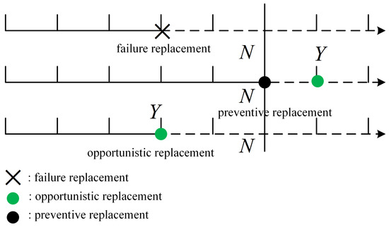
Figure 1. RF discipline.

First of all, according to Figure 1, we can straightforwardly calculate the probability that the item is replaced at time $n(=0,1,2,\dots )$ by

$$h_{fj}\left(n\right)=\left\{\begin{array}{ccc}{f}_Y\left(n\right){\overline{G}}_X(n-1)+g_X\left(n\right){\overline{F}}_Y\left(n\right)\hfill & & 0\le n\le N-1\hfill \\ {\overline{G}}_X(N-1){\overline{F}}_Y(N-1)\hfill & & n=N\hfill \\ 0\hfill & & n\ge N+1,\hfill \end{array}\right.$$

(1)

where ${\sum }_{n=0}^{\infty }{h}_{fj}\left(n\right)=1$.

Next, we can calculate the NPV of one unit cost during the renewal cycle:

$$L_f\left(N\right)=\sum _{n=1}^{N-1}{\beta }^n\left[f_Y\left(n\right)\overline{G}(n-1)+g_X\left(n\right){\overline{F}}_Y\left(n\right)\right]+{\beta }^N{\overline{G}}_X(N-1){\overline{F}}_Y(N-1),$$

(2)

where $L_f\left(N\right)$ for Model j are all the same.

We can compute the expected total discounted costs during the renewal cycle, $C_{fj}\left(N\right)$, for Model $j(=1,\cdots ,6)$:

$$\begin{array}{ccc}\hfill C_{f1}\left(N\right)& =& c_F\sum _{n=1}^{N-1}{\beta }^n{f}_Y\left(n\right)\overline{G}(n-1)+c_Y\sum _{n=1}^{N-1}{\beta }^n{g}_X\left(n\right){\overline{F}}_Y\left(n\right)\hfill \\ & +& c_T{\beta }^N{\overline{G}}_X(N-1){\overline{F}}_Y(N-1),\hfill \end{array}$$

(3)

$$\begin{array}{ccc}\hfill C_{f2}\left(N\right)& =& c_F\sum _{n=1}^N{\beta }^n{f}_Y\left(n\right)\overline{G}(n-1)+c_Y\sum _{n=1}^{N-1}{\beta }^n{g}_X\left(n\right){\overline{F}}_Y\left(n\right)\hfill \\ & +& c_T{\beta }^N{\overline{G}}_X(N-1){\overline{F}}_Y\left(N\right),\hfill \end{array}$$

(4)

$$\begin{array}{ccc}\hfill C_{f3}\left(N\right)& =& c_F\sum _{n=1}^{N-1}{\beta }^n{f}_Y\left(n\right)\overline{G}\left(n\right)+c_Y\sum _{n=1}^{N-1}{\beta }^n{g}_X\left(n\right){\overline{F}}_Y(n-1)\hfill \\ & +& c_T{\beta }^N{\overline{G}}_X(N-1){\overline{F}}_Y(N-1),\hfill \end{array}$$

(5)

$$\begin{array}{ccc}\hfill C_{f4}\left(N\right)& =& c_F\sum _{n=1}^{N-1}{\beta }^n{f}_Y\left(n\right)\overline{G}\left(n\right)+c_Y\sum _{n=1}^N{\beta }^n{g}_X\left(n\right){\overline{F}}_Y(n-1)\hfill \\ & +& c_T{\beta }^N{\overline{G}}_X\left(N\right){\overline{F}}_Y(N-1),\hfill \end{array}$$

(6)

$$\begin{array}{ccc}\hfill C_{f5}\left(N\right)& =& c_F\sum _{n=1}^N{\beta }^n{f}_Y\left(n\right)\overline{G}(n-1)+c_Y\sum _{n=1}^N{\beta }^n{g}_X\left(n\right){\overline{F}}_Y\left(n\right)\hfill \\ & +& c_T{\beta }^N{\overline{G}}_X\left(N\right){\overline{F}}_Y\left(N\right),\hfill \end{array}$$

(7)

$$\begin{array}{ccc}\hfill C_{f6}\left(N\right)& =& c_F\sum _{n=1}^N{\beta }^n{f}_Y\left(n\right)\overline{G}\left(n\right)+c_Y\sum _{n=1}^N{\beta }^n{g}_X\left(n\right){\overline{F}}_Y(n-1)\hfill \\ & +& c_T{\beta }^N{\overline{G}}_X\left(N\right){\overline{F}}_Y\left(N\right),\hfill \end{array}$$

(8)

where discount factor $\beta (>0)$ represents the NPV of a unit cost component. In RF discipline, $T{C}_{fj}\left(N\right)$ denotes the NPV of the expected total discounted cost over an infinite time horizon. Then, we have

$$T{C}_{fj}\left(N\right)=\frac{C_{fj}\left(N\right)}{1-L_f\left(N\right)},$$

(9)

for Model $j(=1,\cdots ,6)$ (for the derivation of Equation (1), see Appendix A.1).

Then, the problem is to determine the optimal prescheduled preventive replacement times $N^{*}$ by minimizing $T{C}_{fj}\left(N\right)$.

3.3. Expected Total Cost under RL Discipline

As is shown in Figure 2, RL discipline is described that the replacement is performed at the failure time or one of two preventive replacement times (scheduled replacement time N and opportunistic replacement Y), whichever occurs last. Similarly to the RF discipline, we compute the probabilities that the item is replaced at time $n(=0,1,2,\dots )$ for Model $j(=1,2,\dots ,6)$:

$$h_{lj}\left(n\right)=\left\{\begin{array}{ccc}{f}_Y\left(n\right)\hfill & & 0\le n\le N-1\hfill \\ f_Y\left(N\right){\overline{G}}_X(N-1)+{\overline{F}}_Y(N-1)\hfill \\ \times G_X(N-1)+{\overline{F}}_Y\left(N\right)g_X\left(N\right)\hfill & & n=N\hfill \\ f_Y\left(n\right){\overline{G}}_X(n-1)+g_X\left(n\right){\overline{F}}_Y\left(n\right)\hfill & & n\ge N+1,\hfill \end{array}\right.$$

(10)

where ${\sum }_{n=0}^{\infty }{h}_{lj}\left(n\right)=1$.

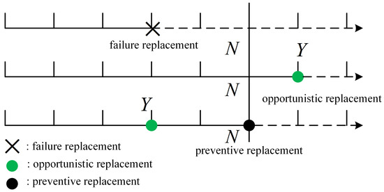
Figure 2. RL discipline.

Similarly to RF discipline, the values of $L_l\left(N\right)$ are all the same for Model $j(=1,\cdots ,6)$, so we can obtain

$$L_l\left(N\right)=\sum _{n=1}^{N-1}{\beta }^n{f}_Y\left(n\right)+{\beta }^N{\overline{F}}_Y(N-1)G_X(N-1)+\sum _{n=N}^{\infty }{\beta }^n\left[f_Y\left(n\right)\overline{G}(n-1)+{\overline{F}}_Y\left(n\right)g_X\left(n\right)\right].$$

(11)

We can obtain the expected total discounted over an infinite horizon, $C_{lj}\left(N\right)$, for Model $j(=1,\cdots ,6)$:

$$\begin{array}{ccc}\hfill C_{l1}\left(N\right)& =& c_F\sum _{n=1}^{N-1}{\beta }^n{f}_Y\left(n\right)+c_T{\beta }^N{G}_X(N-1){\overline{F}}_Y(N-1)\hfill \\ & +& c_F\sum _{n=N}^{\infty }{\beta }^n{f}_Y\left(n\right){\overline{G}}_X(n-1)+c_Y\sum _{n=N}^{\infty }{\beta }^n{g}_X\left(n\right){\overline{F}}_X\left(n\right),\hfill \end{array}$$

(12)

$$\begin{array}{ccc}\hfill C_{l2}\left(N\right)& =& C_{l5}\left(N\right)=c_F\sum _{n=1}^N{\beta }^n{f}_Y\left(n\right)+c_T{\beta }^N{G}_X(N-1){\overline{F}}_Y\left(N\right)\hfill \\ & +& c_F\sum _{n=N+1}^{\infty }{\beta }^n{f}_Y\left(n\right){\overline{G}}_X(n-1)+c_Y\sum _{n=N}^{\infty }{\beta }^n{g}_X\left(n\right){\overline{F}}_X\left(n\right),\hfill \end{array}$$

(13)

$$\begin{array}{ccc}\hfill C_{l3}\left(N\right)& =& C_{l4}\left(N\right)=c_F\sum _{n=1}^{N-1}{\beta }^n{f}_Y\left(n\right)+c_T{\beta }^N{G}_X(N-1){\overline{F}}_Y(N-1)\hfill \\ & +& c_F\sum _{n=N}^{\infty }{\beta }^n{f}_Y\left(n\right){\overline{G}}_X\left(n\right)+c_Y\sum _{n=N}^{\infty }{\beta }^n{g}_X\left(n\right){\overline{F}}_X(n-1),\hfill \end{array}$$

(14)

$$\begin{array}{ccc}\hfill C_{l6}\left(N\right)& =& c_F\sum _{n=1}^{N-1}{\beta }^n{f}_Y\left(n\right)+c_F{\beta }^N{f}_Y\left(N\right)\left[1-g_X\left(N\right)\right]+c_T{\beta }^N{G}_X(N-1){\overline{F}}_Y\left(N\right)\hfill \\ & +& c_F\sum _{n=N+1}^{\infty }{\beta }^n{f}_Y\left(n\right){\overline{G}}_X\left(n\right)+c_Y\sum _{n=N}^{\infty }{\beta }^n{g}_X\left(n\right){\overline{F}}_X(n-1).\hfill \end{array}$$

(15)

Then, the problem is to minimize the expected total costs over an infinite horizon:

$$T{C}_{lj}=\frac{C_{lj}\left(N\right)}{1-L_l\left(N\right)}.$$

(16)

Our interest is to find the optimal prescheduled preventive replacement times $N^{*}$, which minimize $T{C}_{lj}\left(N\right)$.

4. Model Formulation

4.1. RF Policies

We determine the optimal prescheduled preventive replacement times $N^{*}$, which minimize $T{C}_{fj}\left(N\right)$ for Model $j(=1,\cdots ,6)$ under RF discipline. When computing the difference in $T{C}_{fj}\left(N\right)$ for a fixed $\beta$, we have

$$T{C}_{fj}(N+1)-T{C}_{fj}\left(N\right)=\frac{{\overline{F}}_Y\left(N\right){\overline{G}}_X\left(N\right)}{\left[1-L_f(N+1)\right]\left[1-L_f\left(N\right)\right]}{w}_{fj}(N\mid \beta ),$$

(17)

in which

$$\begin{array}{ccc}\hfill w_{f1}(N\mid \beta )& =& \left[\frac{\left(c_F-c_T\right){\Lambda }_Y\left(N\right)\left[1+{\Phi }_X\left(N\right)\right]}{1-\beta }-\frac{\left(c_T-c_Y\right){\Phi }_X\left(N\right)}{1-\beta }-c_T\right]\left[1-L_f\left(N\right)\right]\hfill \\ & -& C_{f1}\left(N\right),\hfill \end{array}$$

(18)

$$\begin{array}{c}\hfill w_{f2}(N\mid \beta )=\left[\frac{\beta \left(c_F-c_T\right){\lambda }_Y(N+1)}{1-\beta }-\frac{\left(c_T-c_Y\right){\Phi }_X\left(N\right)}{1-\beta }-c_T\right]\left[1-L_f\left(N\right)\right]-C_{f2}\left(N\right),\end{array}$$

(19)

$$\begin{array}{ccc}\hfill w_{f3}(N\mid \beta )& =& \left[\frac{\left(c_F-c_T\right){\Lambda }_Y\left(N\right)}{1-\beta }-\frac{\left(c_T-c_Y\right){\Phi }_X\left(N\right)\left[{\Lambda }_Y\left(N\right)+1\right]}{1-\beta }-c_T\right]\left[1-L_f\left(N\right)\right]\hfill \\ & -& C_{f13}\left(N\right),\hfill \end{array}$$

(20)

$$\begin{array}{c}\hfill w_{f4}(N\mid \beta )=\left[\frac{\left(c_F-c_T\right){\Lambda }_Y\left(N\right)}{1-\beta }-\frac{\beta \left(c_T-c_Y\right){\varphi }_X(N+1)}{1-\beta }-c_T\right]\left[1-L_f\left(N\right)\right]-C_{f4}\left(N\right),\end{array}$$

(21)

$$\begin{array}{ccc}\hfill w_{f5}(N\mid \beta )& =& \left[\frac{\beta \left(c_F-c_T\right){\lambda }_Y(N+1)}{1-\beta }-\frac{\beta \left(c_T-c_Y\right){\varphi }_X(N+1)\left[1-{\lambda }_Y(N+1)\right]}{1-\beta }-c_T\right]\hfill \\ & \times & \left[1-L_f\left(N\right)\right]-C_{f5}\left(N\right),\hfill \end{array}$$

(22)

$$\begin{array}{ccc}\hfill w_{f6}(N\mid \beta )& =& \left[\frac{\beta \left(c_F-c_T\right){\lambda }_Y(N+1)\left[1-{\varphi }_X(N+1)\right]}{1-\beta }-\frac{\beta \left(c_T-c_Y\right){\varphi }_X(N+1)}{1-\beta }-c_T\right]\hfill \\ & \times & \left[1-L_f\left(N\right)\right]-C_{f6}\left(N\right).\hfill \end{array}$$

(23)

It has been proven that the function ${\Lambda }_Y\left(n\right)\left({\Phi }_X\left(n\right)\right)$ is strictly increasing (decreasing) in n, if and only if ${\lambda }_Y\left(n\right)\left({\varphi }_X\left(n\right)\right)$ is strictly increasing (decreasing) in n (see Wu et al. [4]). In addition, see Appendix A.2 for the monotonicity of functions $w_{fj}(N\mid \beta )(j=1,\cdots ,6)$.

We determine the optimal prescheduled preventive replacement times $N^{*}$ that minimize the expected costs over an infinite time horizon, $T{C}_{fj}\left(N\right)$, for Model $j(=1,\cdots ,6)$.

Theorem 1.

(i) 

Suppose that $w_{fj}(N\mid \beta )$ is a strictly increasing function of N for a fixed β:

(1) 

If $w_{fj}(\infty \mid \beta )>0$, then there exists at least one (at most two) optimal prescheduled preventive replacement time $N^{*}$, which satisfies $w_{fj}(N^{*}-1\mid \beta )<0$ and $w_{fj}(N^{*}\mid \beta )\ge 0$.

(2) 

If $w_{fj}(\infty \mid \beta )\le 0$, then the optimal prescheduled preventive replacement time is given by $N^{*}\to \infty$, and so the failure replacement or opportunistic replacement is better than the preventive replacement.

(ii) 

If $w_{fj}(N\mid \beta )$ is a decreasing function of N, the optimal prescheduled preventive replacement time is always $N^{*}\to \infty$ or $N^{*}=1$.

For the proof of Theorem 1, see the Appendix A.3.

We can derive the results directly from Theorem 1 as follows.

Theorem 2.

For Model $j(=1,\cdots ,6)$, suppose that $w_{fj}(N\mid \beta )$ is a strictly increasing function and $w_{fj}(N\mid \beta )>0$, under Assumption 1. Then, the minimum expected total discounted costs over an infinite horizon have the following lower and upper bounds:

$$V_{fj}(N^{*}-1)<T{C}_{fj}\left(N^{*}\right)\le V_{fj}\left(N^{*}\right),$$

(24)

where

$$V_{f1}\left(N\right)=\frac{\left(c_F-c_T\right){\Lambda }_Y\left(N\right)\left[1+{\Phi }_X\left(N\right)\right]}{1-\beta }-\frac{\left(c_T-c_Y\right){\Phi }_X\left(N\right)}{1-\beta }-c_T,$$

(25)

$$V_{f2}\left(N\right)=\frac{\beta \left(c_F-c_T\right){\lambda }_Y(N+1)}{1-\beta }-\frac{\left(c_T-c_Y\right){\Phi }_X\left(N\right)}{1-\beta }-c_T,$$

(26)

$$V_{f3}\left(N\right)=\frac{\left(c_F-c_T\right){\Lambda }_Y\left(N\right)}{1-\beta }-\frac{\left(c_T-c_Y\right){\Phi }_X\left(N\right)\left[1+{\Lambda }_Y\left(N\right)\right]}{1-\beta }-c_T,$$

(27)

$$V_{f4}\left(N\right)=\frac{\left(c_F-c_T\right){\Lambda }_Y\left(N\right)}{1-\beta }-\frac{\beta \left(c_T-c_Y\right){\varphi }_X(N+1)}{1-\beta }-c_T,$$

(28)

$$V_{f5}\left(N\right)=\frac{\beta \left(c_F-c_T\right){\lambda }_Y(N+1)}{1-\beta }-\frac{\beta \left(c_T-c_Y\right){\varphi }_X(N+1)\left[1-{\lambda }_Y(N+1)\right]}{1-\beta }-c_T,$$

(29)

$$V_{f6}\left(N\right)=\frac{\beta \left(c_F-c_T\right){\lambda }_Y(N+1)\left[1-{\varphi }_X(N+1)\right]}{1-\beta }-\frac{\beta \left(c_T-c_Y\right){\varphi }_X(N+1)}{1-\beta }-c_T.$$

(30)

4.2. RL Policies

We formulate the optimal preventive replacement times $N^{*}$, which minimize $T{C}_{lj}\left(N\right)$ for Model $j(=1,\cdots ,6)$ with RL discipline. Taking the difference of $T{C}_{lj}\left(N\right)$ with respect to N, we have

$$T{C}_{lj}(N+1)-T{C}_{lj}\left(N\right)=\frac{{\overline{F}}_Y\left(N\right)G_X\left(N\right)}{\left[1-L_l(N+1)\right]\left[1-L_l\left(N\right)\right]}{w}_{lj}(N\mid \beta ),$$

(31)

where

$$\begin{array}{ccc}\hfill w_{l1}(N\mid \beta )& =& \left[\frac{\left(c_F-c_T\right){\Lambda }_Y\left(N\right)\left[1-{\Psi }_X\left(N\right)\right]}{1-\beta }+\frac{\left(c_T-c_Y\right){\Psi }_X\left(N\right)}{1-\beta }-c_T\right]\left[1-L_l\left(N\right)\right]\hfill \\ & -& C_{l1}\left(N\right),\hfill \end{array}$$

(32)

$$\begin{array}{ccc}\hfill w_{l2}(N\mid \beta )& =& w_{l5}(N\mid \beta )=\left[\frac{\beta \left(c_F-c_T\right){\lambda }_Y(N+1)}{1-\beta }+\frac{\left(c_T-c_Y\right){\Psi }_X\left(N\right)}{1-\beta }-c_T\right]\hfill \\ & \times & \left[1-L_l\left(N\right)\right]-C_{l2}\left(N\right),\hfill \end{array}$$

(33)

$$\begin{array}{ccc}\hfill w_{l3}(N\mid \beta )& =& w_{l4}(N\mid \beta )=\left[\frac{\left(c_F-c_T\right){\Lambda }_Y\left(N\right)}{1-\beta }+\frac{\left(c_T-c_Y\right){\Psi }_X\left(N\right)\left[1+{\Lambda }_Y\left(N\right)\right]}{1-\beta }-c_T\right]\hfill \\ & \times & \left[1-L_l\left(N\right)\right]-C_{l3}\left(N\right),\hfill \end{array}$$

(34)

$$\begin{array}{ccc}\hfill w_{l6}(N\mid \beta )& =& [\frac{\left(c_F-c_T\right)\left[{\Lambda }_Y\left(N\right){\Phi }_X\left(N\right)+\beta {\lambda }_Y(N+1)\right]}{1-\beta }\hfill \\ & +& \frac{\left(c_T-c_Y\right){\Psi }_X\left(N\right)\left[1+{\Lambda }_Y\left(N\right)\right]}{1-\beta }-c_T]\hfill \\ & \times & \left[1-L_l\left(N\right)\right]-C_{l6}\left(N\right).\hfill \end{array}$$

(35)

Taking the subsequent difference of $w_{lj}(N\mid \beta )$ for $j=1,\cdots ,6$ in Equations (32)–(35), we can obtain

$$\begin{array}{ccc}\hfill w_{l1}(N+1\mid \beta )-w_{l1}(N\mid \beta )& =& \{\frac{\left(c_F-c_T\right)[{\Lambda }_Y(N+1)\left[1-{\Psi }_X(N+1)\right]}{1-\beta }\hfill \\ & -& \frac{{\Lambda }_Y\left(N\right)\left[1-{\Psi }_X\left(N\right)\right]]}{1-\beta }\hfill \\ & +& \frac{\left(c_T-c_Y\right)\left[{\Psi }_X(N+1)-{\Psi }_X\left(N\right)\right]}{1-\beta }\}\hfill \\ & \times & \left[1-L_l(N+1)\right],\hfill \end{array}$$

(36)

$$\begin{array}{ccc}\hfill w_{l2}(N+1\mid \beta )-w_{l2}(N\mid \beta )& =& w_{l5}(N+1\mid \beta )-w_{l5}(N\mid \beta )\hfill \\ & =& \{\frac{\beta \left(c_F-c_T\right)\left[{\lambda }_Y(N+2)-{\Lambda }_Y(N+1)\right]}{1-\beta }\hfill \\ & +& \frac{\left(c_T-c_Y\right)\left[{\Psi }_X(N+1)-{\Psi }_X\left(N\right)\right]}{1-\beta }]\hfill \\ & \times & \left[1-L_l(N+1)\right],\hfill \end{array}$$

(37)

$$\begin{array}{ccc}\hfill w_{l3}(N+1\mid \beta )-w_{l3}(N\mid \beta )& =& w_{l4}(N+1\mid \beta )-w_{l4}(N\mid \beta )\hfill \\ & =& \{\frac{\left(c_F-c_T\right)\left[{\Lambda }_Y(N+1)-{\Lambda }_Y\left(N\right)\right]}{1-\beta }\hfill \\ & +& \frac{\left(c_T-c_Y\right)[{\Psi }_X(N+1)\left(1+{\Lambda }_Y(N+1)\right)}{1-\beta }\hfill \\ & -& \frac{{\Psi }_X\left(N\right)\left(1+{\Lambda }_Y\left(N\right)\right)]}{1-\beta }\}\hfill \\ & \times & \left[1-L_l(N+1)\right],\hfill \end{array}$$

(38)

$$\begin{array}{ccc}\hfill w_{l6}(N+1\mid \beta )-w_{l6}(N\mid \beta )& =& \{\frac{\left(c_F-c_T\right)[{\Lambda }_Y(N+1){\Psi }_X(N+1)-{\Lambda }_Y\left(N\right){\Psi }_X\left(N\right)}{1-\beta }\hfill \\ & +& \frac{\beta {\lambda }_Y(N+2)-\beta {\lambda }_Y(N+1)]}{1-\beta }\hfill \\ & +& \frac{\left(c_T-c_Y\right)[{\Psi }_X(N+1)\left(1+{\Lambda }_Y(N+1)\right)}{1-\beta }\hfill \\ & -& \frac{{\Psi }_X\left(N\right)\left(1+{\Lambda }_Y\left(N\right)\right)]}{1-\beta }\}\left[1-L_l(N+1)\right].\hfill \end{array}$$

(39)

From Equations (36)–(39), the monotone properties of $w_{lj}(N\mid \beta )(j=1,\cdots ,6)$ depend on the ${\Lambda }_Y\left(N\right)$ and the cost parameters in our modeling. It was proven in [4] that if the lifetime X decreases, then the ${\Phi }_X\left(N\right)$ decreases in N. The necessary conditions that $w_{lj}(N\mid \beta )(j=1,\cdots ,6)$ is a strictly increasing function of N are given in Appendix A.4.

Theorem 3.

(i) 

Suppose that $w_{lj}(N\mid \beta )$ is a strictly increasing function of N for a fixed β:

(1) 

If $w_{lj}(\infty \mid \beta )>0$, then there exists at least one (at most two) optimal prescheduled preventive replacement time $N^{*}$, which satisfies $w_{lj}(N^{*}-1\mid \beta )<0$ and $w_{lj}(N^{*}\mid \beta )\ge 0$.

(2) 

If $w_{lj}(\infty \mid \beta )\le 0$, then the optimal prescheduled preventive replacement time is given by $N^{*}\to \infty$, and so the optimal prescheduled preventive replacement is only to perform the failure replacement.

(ii) 

If $w_{lj}(N\mid \beta )$ is a decreasing function of N, the optimal prescheduled preventive replacement time is always $N^{*}\to \infty$ or $N^{*}=1$.

For the proof of Theorem 3, see the Appendix A.3.

We can directly have the following result from Theorem 3.

Theorem 4.

For Model $j(=1,\cdots ,6)$, suppose that $w_{lj}(N\mid \beta )$ is a strictly increasing function and $w_{lj}(N\mid \beta )>0$, under Assumption 1. Then, the minimum expected total discounted costs over an infinite horizon have the following lower and upper bounds:

$$V_{lj}(N^{*}-1)<T{C}_{lj}\left(N^{*}\right)\le V_{lj}\left(N^{*}\right),$$

(40)

where

$$V_{l1}\left(N\right)=\frac{\left(c_F-c_T\right){\Lambda }_Y\left(N\right)\left[1-{\Psi }_X\left(N\right)\right]}{1-\beta }+\frac{\left(c_T-c_Y\right){\Psi }_X\left(N\right)}{1-\beta }-c_T,$$

(41)

$$V_{l2}\left(N\right)=V_{l5}\left(N\right)=\frac{\beta \left(c_F-c_T\right){\lambda }_Y(N+1)}{1-\beta }+\frac{\left(c_T-c_Y\right){\Psi }_X\left(N\right)}{1-\beta }-c_T,$$

(42)

$$V_{l3}\left(N\right)=V_{l4}\left(N\right)=\frac{\left(c_F-c_T\right){\Lambda }_Y\left(N\right)}{1-\beta }+\frac{\left(c_T-c_Y\right){\Psi }_X\left(N\right)\left[1+{\Lambda }_Y\left(N\right)\right]}{1-\beta }-c_T,$$

(43)

$$V_{l6}\left(N\right)=\frac{\left(c_F-c_T\right)\left[{\Lambda }_Y\left(N\right){\Psi }_X\left(N\right)+\beta {\lambda }_Y(N+1)\right]}{1-\beta }+\frac{\left(c_T-c_Y\right){\Psi }_X\left(N\right)\left[1+{\Phi }_X\left(N\right)\right]}{1-\beta }-c_T.$$

(44)

5. Unified Models with Probabilistic Priority

In the preceding discussion concerning RF and RL policies, we categorized six priority cases and determined the optimal scheduled preventive replacement times for each scenario. Nevertheless, it is essential to acknowledge that the prioritization of replacement is not invariably fixed. In other words, the assignment of priority is subject to probabilistic variation and may shift at each replacement decision juncture. In unified modeling, let $p_j(0\le p_j<1)$ denote the probability that each priority Model $j(=1,\cdots ,6)$ occurs, where ${\sum }_{j=1}^6{p}_j=1$.

First, we calculate the unified model under RF discipline. Since the $L_f\left(N\right)$ for Model $j(=1,\cdots ,6)$ are all the same, $L_f\left(N\right)$ in the unified model with probability $p_j$ is given by $L_{f7}\left(N\right)=L_f\left(N\right)$ in Equation (2). In addition, the total expected discounted costs during the renewal cycle can be calculated by $C_{f7}\left(N\right)={\sum }_{j=1}^6{p}_j{C}_{fj}\left(N\right)$ with Equations (3)–(8). The underlying problem can be thought as $mi{n}_{N}T{C}_{f7}\left(N\right)$, where $T{C}_{f7}\left(N\right)=C_{f7}\left(N\right)/\left[1-L_f\left(N\right)\right]$.

We define $w_{f7}(N\mid \beta )={\sum }_{j=1}^6{p}_j{V}_{fj}\left(N\right)L_f\left(N\right)-C_{fj}\left(N\right)$ with Equations (25)–(30). Then, we can obtain that $w_{f7}(N+1\mid \beta )-w_{f7}(N\mid \beta )={\sum }_{j=1}^6{p}_j\left\{w_{f7}(N+1\mid \beta )-\right.$$\left.w_{f7}(N\mid \beta )\right\}{L}_f\left(N\right)-C_{fj}\left(N\right)$. Therefore, for $p_j\ne 0$, necessary conditions of strictly increasing $w_{f7}(N\mid \beta )$ for a given equation are to hold all conditions in Appendix A.2 under Assumption 1. In a unified model, we, when in position, can have the optimal preventive replacement policies under RF discipline as follows.

Theorem 5.

Suppose that $w_{f7}(0\mid \beta )<0$ and $w_{f7}(\infty \mid \beta )>0$ for a given β, under Assumption 1. Then, the expected total discounted cost over an infinite horizon has the following lower and upper bounds:

$$V_{f7}(N^{*}-1)<T{C}_{f7}\left(N^{*}\right)\le V_{f7}\left(N^{*}\right),$$

(45)

where

$$V_{f7}=\sum _{j=1}^6{p}_j{V}_{fj}\left(N\right).$$

(46)

Next, we examine the unified RL model. Since the net present value (NPV) of one unit cost during the renewal cycle, denoted as $L_f\left(N\right)$ for Model $j(=1,\cdots ,6)$, remains constant, the expression for $L_l\left(N\right)$ in the unified model, accounting for probability $p_j$, is equivalent to $L_{l7}\left(N\right)=L_l\left(N\right)$ as defined in Equation (11). Consequently, the total expected discounted costs throughout the renewal cycle can be determined by $C_{l7}\left(N\right)={\sum }_{j=1}^6{p}_j{C}_{lj}\left(N\right)$ using Equations (12)–(15). The underlying problem can be thought as $mi{n}_{N}T{C}_{l7}\left(N\right)$, where $T{C}_{l7}\left(N\right)=C_{l7}\left(N\right)/\left[1-L_l\left(N\right)\right]$. Define $w_{l7}(N\mid \beta )={\sum }_{j=1}^6{p}_j{V}_{lj}\left(N\right)L_l\left(N\right)-C_{lj}\left(N\right)$ with Equations (41)–(44). Then, we can obtain that $w_{l7}(N+1\mid \beta )-w_{l7}(N\mid \beta )={\sum }_{j=1}^6{p}_j\left\{w_{f7}(N+1\mid \beta )-w_{f7}(N\mid \beta )\right\}{L}_f\left(N\right)-C_{fj}\left(N\right)$. The necessary conditions of strictly increasing $w_{l7}(N\mid \beta )$ for a given equation are to hold all conditions in Appendix A.4 under Assumption 1. In a unified model, we, when in position, can have the optimal preventive replacement policies under RL discipline, as follows.

Theorem 6.

Suppose that $w_{l7}(0\mid \beta )<0$ and $w_{l7}(\infty \mid \beta )>0$ for a given β, under Assumption 1. Then, the expected total discounted cost over an infinite horizon has the following lower and upper bounds:

$$V_{l7}(N^{*}-1)<T{C}_{l7}\left(N^{*}\right)\le V_{l7}\left(N^{*}\right),$$

(47)

where

$$V_{l7}=\sum _{j=1}^6{p}_j{V}_{lj}\left(N\right).$$

(48)

6. Numerical Illustrations and Discussion

Based on the previous theorems, here, we give a case study to compare RF policies with RL policies in discrete time. As we know, the pole air switch is a kind of long-life product and is distributed to some regions for the poles. In a similar case, Holland and McLean [32] studied the electrical devices used in a continuous time replacement model. Wu et al. [4] first formulated the discrete time optimal preventive replacement times using the failure data of pole air switch in the past 25 years in Hiroshima city. Then, Wu et al. [31] further studied the age-based and opportunity-based age replacement policies in [4]. In this paper, we take the same model parameters as those of Wu et al. [4,31].

In Wu et al.’s study [4,31], the authors calculated that the failure time distribution is given by the discrete Weibull distribution $f_Y\left(n\right)=k^{{(n-1)}^a}-k^{n^a}$, with the failure rate ${\lambda }_Y\left(n\right)=1-k^{{(n-1)}^a-n^a}$, where $k=0.9995$ and $a=2.8547$. Also, it is assumed that the opportunity arrival time obeys the geometric distribution $g_X\left(n\right)=q^{(n-1)}-q^n$ with $q=0.95$. In this paper, we set the cost parameters as $c_F=2.0,3.0,4.0,5.0,6.0,7.0,8.0,9.0,10.0,11.0$ (K dollar), $c_T=1$ (K dollar), $c_Y=0.4,1$ (K dollar). The discounted factor is set as $\beta =0.8,0.9.$ In a unified model, the probabilistic parameters are set as $p_1=p_2=p_3=p_4=0.2$, $p_5=p_6=0.1$. In this numerical illustration, we mainly discuss the following questions:

$Q_1$

How does replacement priority influence the optimal prescheduled preventive replacement times?

$Q_2$

How does the failure replacement cost $c_F$ affect the optimal prescheduled preventive replacement times?

$Q_3$

What impact does the opportunistic replacement cost $c_Y$ have on the optimal prescheduled preventive replacement times?

$Q_4$

Which policy is preferable between RF and RL policies?

$Q_5$

What are the differences between the unified model and the deterministic priority models?

$Q_6$

How does the economic environment influence the optimal prescheduled preventive replacement times?

To answer $Q_1$ to $Q_5$, we derive the optimal prescheduled preventive replacement times $N^{*}$ and their associated expected discounted costs $TC\left(N^{*}\right)$ under RF and RL disciplines for each model, when $c_T=1$, $c_Y=0.4,1$ and discounted factor $\beta =0.9$. The results are presented in Table 1, Table 2, Table 3, Table 4, Table 5, Table 6 and Table 7:

Table 1. Optimal prescheduled preventive times $N^{*}$ and associated expected discounted costs $TC\left(N^{*}\right)$ with Model 1, when $\beta =0.9$.

	${\mathit{c}}_{\mathit{Y}}\mathbf{=}\mathbf{0.4}$				${\mathit{c}}_{\mathit{Y}}=1.0$
	RF		RL		RF		RL
${\mathit{c}}_{\mathit{F}}$	${\mathit{N}}^{*}$	${\mathit{TC}}_{\mathit{f}\mathbf{1}}\left({\mathit{N}}^{*}\right)$	${\mathit{N}}^{*}$	${\mathit{TC}}_{\mathit{l}\mathbf{1}}\left({\mathit{N}}^{*}\right)$	${\mathit{N}}^{*}$	${\mathit{TC}}_{\mathit{f}\mathbf{1}}\left({\mathit{N}}^{*}\right)$	${\mathit{N}}^{*}$	${\mathit{TC}}_{\mathit{l}\mathbf{1}}\left({\mathit{N}}^{*}\right)$
2.0	15	0.7585	13	$0.7512$	14	1.0184	13	$0.7583$
3.0	11	0.9750	10	$1.0584$	11	1.2320	11	$1.0793$
4.0	9	1.1439	$9$	$1.3512$	9	1.3971	10	$1.3816$
5.0	8	1.2820	$8$	$1.6388$	8	1.5321	$9$	$1.6768$
6.0	8	1.3952	$8$	$1.9252$	8	1.6453	$9$	$1.9681$
7.0	7	1.4986	$7$	$2.2116$	7	1.7445	$8$	$2.2582$
8.0	7	1.5869	$7$	$2.4955$	7	1.8328	$8$	$2.5546$
9.0	7	1.6753	$7$	$2.7794$	7	1.9211	$8$	$2.8310$
10.0	6	1.7484	$7$	$3.0633$	6	1.9882	$8$	$3.1174$
11.0	6	1.8131	$7$	$3.3472$	6	2.0529	$7$	$3.4092$

Table 2. Optimal prescheduled preventive times $N^{*}$ and associated expected discounted costs $TC\left(N^{*}\right)$ with Model 2, when $\beta =0.9$.

	${\mathit{c}}_{\mathit{Y}}=0.4$				${\mathit{c}}_{\mathit{Y}}=1.0$
	RF		RL		RF		RL
${\mathit{c}}_{\mathit{F}}$	${\mathit{N}}^{*}$	${\mathit{TC}}_{\mathit{f}\mathbf{2}}\left({\mathit{N}}^{*}\right)$	${\mathit{N}}^{*}$	${\mathit{TC}}_{\mathit{l}\mathbf{2}}\left({\mathit{N}}^{*}\right)$	${\mathit{N}}^{*}$	${\mathit{TC}}_{\mathit{f}\mathbf{2}}\left({\mathit{N}}^{*}\right)$	${\mathit{N}}^{*}$	${\mathit{TC}}_{\mathit{l}\mathbf{2}}\left({\mathit{N}}^{*}\right)$
2.0	17	0.7699	13	$0.7643$	16	1.0305	15	$0.7697$
3.0	12	1.0245	10	$1.0714$	12	1.2827	11	$1.1067$
4.0	10	1.2305	$9$	$1.3705$	10	1.4859	10	$1.4208$
5.0	9	1.4501	$8$	$1.6697$	9	1.6538	$9$	$1.7243$
6.0	8	1.5551	$7$	$1.9688$	8	1.8053	$8$	$2.0229$
7.0	7	1.6920	$6$	$2.2601$	7	1.9378	$8$	$2.3195$
8.0	7	1.8125	$6$	$2.5499$	7	2.0584	$7$	$2.6151$
9.0	7	1.9931	$6$	$2.8297$	6	2.1737	$7$	$2.9072$
10.0	6	2.0299	$6$	$3.1295$	6	2.2697	$7$	$3.1994$
11.0	6	2.2159	$6$	$3.4297$	6	2.3657	$7$	$3.4915$

Table 3. Optimal prescheduled preventive times $N^{*}$ and associated expected discounted costs $TC\left(N^{*}\right)$ with Model 3, when $\beta =0.9$.

	${\mathit{c}}_{\mathit{Y}}=0.4$				${\mathit{c}}_{\mathit{Y}}=1.0$
	RF		RL		RF		RL
${\mathit{c}}_{\mathit{F}}$	${\mathit{N}}^{*}$	${\mathit{TC}}_{\mathit{f}\mathbf{3}}\left({\mathit{N}}^{*}\right)$	${\mathit{N}}^{*}$	${\mathit{TC}}_{\mathit{l}\mathbf{3}}\left({\mathit{N}}^{*}\right)$	${\mathit{N}}^{*}$	${\mathit{TC}}_{\mathit{f}\mathbf{3}}\left({\mathit{N}}^{*}\right)$	${\mathit{N}}^{*}$	${\mathit{TC}}_{\mathit{l}\mathbf{3}}\left({\mathit{N}}^{*}\right)$
2.0	15	0.7679	12	$0.7449$	15	1.0058	14	$0.7558$
3.0	11	0.9507	10	$1.0325$	11	1.2134	11	$1.0686$
4.0	10	1.1153	8	$1.3178$	10	1.3757	10	$1.3621$
5.0	9	1.2504	$7$	$1.5960$	9	1.5078	$9$	$1.6457$
6.0	8	1.3635	$7$	$1.8694$	8	1.6170	$8$	$1.9262$
7.0	7	1.4695	$7$	$2.1429$	7	1.7180	$8$	$2.2036$
8.0	7	1.5534	$7$	$2.4164$	7	1.8019	$8$	$2.4810$
9.0	7	1.6373	$7$	$2.6899$	7	1.8858	$7$	$2.7581$
10.0	6	1.7173	$6$	$2.9626$	6	1.9591	$7$	$3.0315$
11.0	6	1.7788	$6$	$3.2346$	6	2.0205	$7$	$3.3051$

Table 4. Optimal prescheduled preventive times $N^{*}$ and associated expected discounted costs $TC\left(N^{*}\right)$ with Model 4, when $\beta =0.9$.

	${\mathit{c}}_{\mathit{Y}}=0.4$				${\mathit{c}}_{\mathit{Y}}=1.0$
	RF		RL		RF		RL
${\mathit{c}}_{\mathit{F}}$	${\mathit{N}}^{*}$	${\mathit{TC}}_{\mathit{f}\mathbf{4}}\left({\mathit{N}}^{*}\right)$	${\mathit{N}}^{*}$	${\mathit{TC}}_{\mathit{l}\mathbf{4}}\left({\mathit{N}}^{*}\right)$	${\mathit{N}}^{*}$	${\mathit{TC}}_{\mathit{f}\mathbf{4}}\left({\mathit{N}}^{*}\right)$	${\mathit{N}}^{*}$	${\mathit{TC}}_{\mathit{l}\mathbf{4}}\left({\mathit{N}}^{*}\right)$
2.0	15	0.7658	12	$0.7449$	15	1.0058	14	$0.7558$
3.0	11	0.9434	10	$1.0325$	11	1.2134	11	$1.0686$
4.0	10	1.1057	$9$	$1.3178$	10	1.3757	10	$1.3621$
5.0	9	1.2378	$8$	$1.5960$	9	1.5078	$9$	$1.6457$
6.0	8	1.3470	$7$	$1.8694$	8	1.6170	$8$	$1.9262$
7.0	7	1.4480	$7$	$2.1429$	7	1.7180	$8$	$2.2036$
8.0	7	1.5319	$7$	$2.4164$	7	1.8019	$8$	$2.4810$
9.0	7	1.6158	$7$	$2.6899$	7	1.8858	$7$	$2.7581$
10.0	6	1.6891	$6$	$2.9626$	6	1.9591	$7$	$3.0315$
11.0	6	1.7505	$6$	$3.2346$	6	2.0205	$7$	$3.3051$

Table 5. Optimal prescheduled preventive times $N^{*}$ and associated expected discounted costs $TC\left(N^{*}\right)$ with Model 5, when $\beta =0.9$.

	${\mathit{c}}_{\mathit{Y}}=0.4$				${\mathit{c}}_{\mathit{Y}}=1.0$
	RF		RL		RF		RL
${\mathit{c}}_{\mathit{F}}$	${\mathit{N}}^{*}$	${\mathit{TC}}_{\mathit{f}\mathbf{5}}\left({\mathit{N}}^{*}\right)$	${\mathit{N}}^{*}$	${\mathit{TC}}_{\mathit{l}\mathbf{5}}\left({\mathit{N}}^{*}\right)$	${\mathit{N}}^{*}$	${\mathit{TC}}_{\mathit{f}\mathbf{5}}\left({\mathit{N}}^{*}\right)$	${\mathit{N}}^{*}$	${\mathit{TC}}_{\mathit{l}\mathbf{5}}\left({\mathit{N}}^{*}\right)$
2.0	16	0.7689	13	$0.7643$	16	1.0305	15	$0.7697$
3.0	12	1.0196	10	$1.0714$	12	1.2827	11	$1.1067$
4.0	10	1.2217	9	$1.3705$	10	1.4859	10	$1.4208$
5.0	9	1.3934	$8$	$1.6697$	9	1.6538	$9$	$1.7243$
6.0	8	1.5396	$7$	$1.9688$	8	1.8053	$8$	$2.0229$
7.0	7	1.6714	$6$	$2.2601$	7	1.9378	$8$	$2.3195$
8.0	7	1.7920	$6$	$2.5499$	7	2.0584	$7$	$2.6151$
9.0	6	1.9066	$6$	$2.8297$	6	2.1737	$7$	$2.9072$
10.0	6	2.0026	$6$	$3.1295$	6	2.2697	$7$	$3.1994$
11.0	6	2.0986	$6$	$3.4297$	6	2.3657	$7$	$3.4915$

Table 6. Optimal prescheduled preventive times $N^{*}$ and associated expected discounted costs $TC\left(N^{*}\right)$ with Model 6, when $\beta =0.9$.

	${\mathit{c}}_{\mathit{Y}}=0.4$				${\mathit{c}}_{\mathit{Y}}=1.0$
	RF		RL		RF		RL
${\mathit{c}}_{\mathit{F}}$	${\mathit{N}}^{*}$	${\mathit{TC}}_{\mathit{f}\mathbf{6}}\left({\mathit{N}}^{*}\right)$	${\mathit{N}}^{*}$	${\mathit{TC}}_{\mathit{l}\mathbf{6}}\left({\mathit{N}}^{*}\right)$	${\mathit{N}}^{*}$	${\mathit{TC}}_{\mathit{f}\mathbf{6}}\left({\mathit{N}}^{*}\right)$	${\mathit{N}}^{*}$	${\mathit{TC}}_{\mathit{l}\mathbf{6}}\left({\mathit{N}}^{*}\right)$
2.0	17	0.7463	13	$0.7436$	17	1.0163	14	$0.7778$
3.0	12	0.9896	10	$1.0353$	12	1.2597	10	$1.1641$
4.0	10	1.1872	$8$	$1.3206$	10	1.4572	10	$1.5180$
5.0	9	1.3545	$7$	$1.6058$	9	1.6245	$8$	$1.8438$
6.0	8	1.4990	$7$	$1.8910$	8	1.7690	$7$	$2.1548$
7.0	7	1.6317	$7$	$2.1760$	7	1.9017	$7$	$2.4461$
8.0	7	1.7462	$6$	$2.4611$	7	2.0161	$7$	$2.7313$
9.0	7	1.8607	$6$	$2.7463$	7	2.1307	$6$	$3.0164$
10.0	6	1.9565	$6$	$3.0314$	6	2.2265	$6$	$3.3016$
11.0	6	2.0477	$6$	$3.3165$	6	2.3177	$6$	$3.5867$

Table 7. Optimal prescheduled preventive times $N^{*}$ and associated expected discounted costs $TC\left(N^{*}\right)$ with unified model, when $\beta =0.9$.

	${\mathit{c}}_{\mathit{Y}}=0.4$				${\mathit{c}}_{\mathit{Y}}=1.0$
	RF		RL		RF		RL
${\mathit{c}}_{\mathit{F}}$	${\mathit{N}}^{*}$	${\mathit{TC}}_{\mathit{f}\mathbf{7}}\left({\mathit{N}}^{*}\right)$	${\mathit{N}}^{*}$	${\mathit{TC}}_{\mathit{l}\mathbf{7}}\left({\mathit{N}}^{*}\right)$	${\mathit{N}}^{*}$	${\mathit{TC}}_{\mathit{f}\mathbf{7}}\left({\mathit{N}}^{*}\right)$	${\mathit{N}}^{*}$	${\mathit{TC}}_{\mathit{l}\mathbf{7}}\left({\mathit{N}}^{*}\right)$
2.0	15	0.7524	13	$0.7512$	15	1.0173	15	$0.7663$
3.0	11	0.9807	$9$	$1.0581$	11	1.2431	11	$1.0968$
4.0	10	1.1601	$8$	$1.3472$	10	1.4218	10	$1.4050$
5.0	9	1.3099	$7$	$1.6406$	9	1.5702	$9$	$1.7034$
6.0	8	1.4411	$7$	$1.9242$	8	1.6984	$8$	$1.9974$
7.0	7	1.5519	$7$	$2.2161$	7	1.8076	$8$	$2.2882$
8.0	7	1.6507	$6$	$2.5142$	7	1.9064	$8$	$2.5792$
9.0	7	1.7496	$6$	$2.7989$	7	2.0053	$7$	$2.8672$
10.0	6	1.8328	$6$	$3.0835$	6	2.0898	$7$	$3.1539$
11.0	6	1.9083	$6$	$3.3682$	6	2.1609	$7$	$3.4406$

(1)

In all tables, the optimal prescheduled preventive replacement times for the respective priority models often converge to similar values in most cases. This is primarily since these optimal replacement times are discretized as integer values, and the differences in replacement priorities are not particularly significant.

(2)

When the cost of the corrective replacement $c_F$ is increased, the optimal prescheduled preventive replacement times $N^{*}$ become small. When the cost of repairing or replacing equipment becomes expensive, it means that it is no longer cost-effective to wait for the equipment to break down and then perform emergency repairs. In such situations, it is more economical to perform preventive maintenance, which involves regular maintenance or the replacement of components before they fail.

(3)

When the cost of the opportunistic replacement $c_Y$ rises, the optimal prescheduled preventive replacement times $N^{*}$ become small.

(4)

RL policy is only better than RF policy in some limited cases where the failure replacement cost $c_F$ is relatively small. In our example, only when $c_F=2.0$ is RL policy better than RF policy. Conversely, when $c_F$ is larger and the impact of system failure becomes more remarkable, we can find that RF policies are better than RL.

(5)

Comparing Table 1, Table 2, Table 3, Table 4, Table 5 and Table 6 with Table 7, a slight difference between the deterministic priority models and the probabilistic priority model is seen.

To answer $Q_6$, we calculate the optimal preventive replacement times $N^{*}$ and their associated expected costs $TC\left(N^{*}\right)$ under RF and RL disciplines for each model, when $c_T=1$, $c_Y=0.4,1$ and discounted factor $\beta =0.8$. The results are shown in Table 8, Table 9, Table 10, Table 11, Table 12, Table 13 and Table 14. In addition, the influence of an unstable economic environment on optimal preventive replacement times $N^{*}$ is shown in Figure 3 and Figure 4. Comparing Table 1, Table 2, Table 3, Table 4, Table 5, Table 6 and Table 7 with Table 8, Table 9, Table 10, Table 11, Table 12, Table 13 and Table 14, we can find the following:

Table 8. Optimal prescheduled preventive times $N^{*}$ and associated expected discounted costs $TC\left(N^{*}\right)$ with Model 1, when $\beta =0.8$.

	${\mathit{c}}_{\mathit{Y}}=0.4$				${\mathit{c}}_{\mathit{Y}}=1.0$
	RF		RL		RF		RL
${\mathit{c}}_{\mathit{F}}$	${\mathit{N}}^{*}$	${\mathit{TC}}_{\mathit{f}\mathbf{1}}\left({\mathit{N}}^{*}\right)$	${\mathit{N}}^{*}$	${\mathit{TC}}_{\mathit{l}\mathbf{1}}\left({\mathit{N}}^{*}\right)$	${\mathit{N}}^{*}$	${\mathit{TC}}_{\mathit{f}\mathbf{1}}\left({\mathit{N}}^{*}\right)$	${\mathit{N}}^{*}$	${\mathit{TC}}_{\mathit{l}\mathbf{1}}\left({\mathit{N}}^{*}\right)$
2.0	17	0.2312	15	$0.1868$	16	0.3489	16	$0.1841$
3.0	12	0.3014	12	$0.2639$	12	0.4185	13	$0.2689$
4.0	10	0.3623	10	$0.3352$	10	0.4787	10	$0.3432$
5.0	9	0.4150	$9$	$0.4050$	9	0.5307	$9$	$0.4152$
6.0	8	0.4628	$8$	$0.4722$	8	0.5773	$9$	$0.4845$
7.0	8	0.5036	$8$	$0.5397$	8	0.6181	$8$	$0.5539$
8.0	7	0.5432	$7$	$0.6066$	7	0.6562	$8$	$0.6218$
9.0	7	0.5765	$7$	$0.6739$	7	0.6895	$8$	$0.6890$
10.0	7	0.6098	$7$	$0.7404$	7	0.7227	$8$	$0.7562$
11.0	6	0.6426	$7$	$0.8064$	6	0.7532	$7$	$0.8234$

Table 9. Optimal prescheduled preventive times $N^{*}$ and associated expected discounted costs $TC\left(N^{*}\right)$ with Model 2, when $\beta =0.8$.

	${\mathit{c}}_{\mathit{Y}}=0.4$				${\mathit{c}}_{\mathit{Y}}=1.0$
	RF		RL		RF		RL
${\mathit{c}}_{\mathit{F}}$	${\mathit{N}}^{*}$	${\mathit{TC}}_{\mathit{f}\mathbf{2}}\left({\mathit{N}}^{*}\right)$	${\mathit{N}}^{*}$	${\mathit{TC}}_{\mathit{l}\mathbf{2}}\left({\mathit{N}}^{*}\right)$	${\mathit{N}}^{*}$	${\mathit{TC}}_{\mathit{f}\mathbf{2}}\left({\mathit{N}}^{*}\right)$	${\mathit{N}}^{*}$	${\mathit{TC}}_{\mathit{l}\mathbf{2}}\left({\mathit{N}}^{*}\right)$
2.0	22	0.2317	18	$0.1929$	22	0.3494	20	$0.1931$
3.0	14	0.3070	12	$0.2855$	14	0.4245	13	$0.2868$
4.0	12	0.3770	10	$0.3716$	12	0.4942	11	$0.3755$
5.0	10	0.4407	$8$	$0.4537$	10	0.5571	10	$0.4606$
6.0	9	0.4989	$8$	$0.5334$	9	0.6145	$9$	$0.5429$
7.0	8	0.5530	$7$	$0.6113$	8	0.6676	$8$	$0.6235$
8.0	8	0.6021	$6$	$0.6889$	8	0.7166	$8$	$0.7033$
9.0	7	0.6492	$6$	$0.7652$	7	0.7621	$7$	$0.7821$
10.0	7	0.6915	$6$	$0.8414$	7	0.8044	$7$	$0.8598$
11.0	7	0.7338	$6$	$0.9176$	7	0.8468	$7$	$0.9378$

Table 10. Optimal prescheduled preventive times $N^{*}$ and associated expected discounted costs $TC\left(N^{*}\right)$ with Model 2, when $\beta =0.8$.

	${\mathit{c}}_{\mathit{Y}}=0.4$				${\mathit{c}}_{\mathit{Y}}=1.0$
	RF		RL		RF		RL
${\mathit{c}}_{\mathit{F}}$	${\mathit{N}}^{*}$	${\mathit{TC}}_{\mathit{f}\mathbf{3}}\left({\mathit{N}}^{*}\right)$	${\mathit{N}}^{*}$	${\mathit{TC}}_{\mathit{l}\mathbf{3}}\left({\mathit{N}}^{*}\right)$	${\mathit{N}}^{*}$	${\mathit{TC}}_{\mathit{f}\mathbf{3}}\left({\mathit{N}}^{*}\right)$	${\mathit{N}}^{*}$	${\mathit{TC}}_{\mathit{l}\mathbf{3}}\left({\mathit{N}}^{*}\right)$
2.0	17	0.2253	15	$0.1862$	17	0.3452	16	$0.1882$
3.0	13	0.2982	12	$0.2613$	12	0.4121	13	$0.2676$
4.0	11	0.3519	$9$	$0.3305$	11	0.4704	10	$0.3305$
5.0	10	0.4040	$8$	$0.3976$	9	0.5211	$9$	$0.3976$
6.0	9	0.4495	$7$	$0.4627$	9	0.5666	$8$	$0.4627$
7.0	8	0.4901	$7$	$0.5282$	8	0.6059	$8$	$0.5282$
8.0	8	0.5289	$7$	$0.5925$	7	0.6446	$8$	$0.5925$
9.0	7	0.5622	$7$	$0.6563$	7	0.6762	$8$	$0.6563$
10.0	7	0.5938	$7$	$0.7202$	7	0.7079	$7$	$0.7202$
11.0	7	0.6254	$6$	$0.7845$	7	0.7394	$7$	$0.7845$

Table 11. Optimal prescheduled preventive times $N^{*}$ and associated expected discounted costs $TC\left(N^{*}\right)$ with Model 4, when $\beta =0.8$.

	${\mathit{c}}_{\mathit{Y}}=0.4$				${\mathit{c}}_{\mathit{Y}}=1.0$
	RF		RL		RF		RL
${\mathit{c}}_{\mathit{F}}$	${\mathit{N}}^{*}$	${\mathit{TC}}_{\mathit{f}\mathbf{4}}\left({\mathit{N}}^{*}\right)$	${\mathit{N}}^{*}$	${\mathit{TC}}_{\mathit{l}\mathbf{4}}\left({\mathit{N}}^{*}\right)$	${\mathit{N}}^{*}$	${\mathit{TC}}_{\mathit{f}\mathbf{4}}\left({\mathit{N}}^{*}\right)$	${\mathit{N}}^{*}$	${\mathit{TC}}_{\mathit{l}\mathbf{4}}\left({\mathit{N}}^{*}\right)$
2.0	17	0.2251	15	$0.1862$	17	0.3452	16	$0.1882$
3.0	12	0.2922	12	$0.2613$	12	0.4121	13	$0.2676$
4.0	11	0.3505	$9$	$0.3305$	11	0.4704	10	$0.3305$
5.0	9	0.4011	$8$	$0.3976$	9	0.5211	$9$	$0.3976$
6.0	9	0.4466	$7$	$0.4627$	9	0.5666	$8$	$0.4627$
7.0	8	0.4859	$7$	$0.5282$	8	0.6059	$8$	$0.5282$
8.0	7	0.5246	$7$	$0.5925$	7	0.6446	$8$	$0.5925$
9.0	7	0.5562	$7$	$0.6563$	7	0.6762	$8$	$0.6563$
10.0	7	0.5878	$7$	$0.7202$	7	0.7079	$7$	$0.7202$
11.0	7	0.6194	$6$	$0.7845$	7	0.7394	$7$	$0.7845$

Table 12. Optimal prescheduled preventive times $N^{*}$ and associated expected discounted costs $TC\left(N^{*}\right)$ with Model 5, when $\beta =0.8$.

	${\mathit{c}}_{\mathit{Y}}=0.4$				${\mathit{c}}_{\mathit{Y}}=1.0$
	RF		RL		RF		RL
${\mathit{c}}_{\mathit{F}}$	${\mathit{N}}^{*}$	${\mathit{TC}}_{\mathit{f}\mathbf{5}}\left({\mathit{N}}^{*}\right)$	${\mathit{N}}^{*}$	${\mathit{TC}}_{\mathit{l}\mathbf{5}}\left({\mathit{N}}^{*}\right)$	${\mathit{N}}^{*}$	${\mathit{TC}}_{\mathit{f}\mathbf{5}}\left({\mathit{N}}^{*}\right)$	${\mathit{N}}^{*}$	${\mathit{TC}}_{\mathit{l}\mathbf{5}}\left({\mathit{N}}^{*}\right)$
2.0	21	0.2317	18	$0.1929$	22	0.3494	20	$0.1931$
3.0	14	0.3067	12	$0.2855$	14	0.4245	13	$0.2868$
4.0	11	0.3762	10	$0.3716$	12	0.4942	11	$0.3755$
5.0	10	0.4388	$8$	$0.4537$	10	0.5571	10	$0.4606$
6.0	9	0.4962	$8$	$0.5334$	9	0.6145	$9$	$0.5429$
7.0	8	0.5490	$7$	$0.6113$	8	0.6676	$8$	$0.6235$
8.0	8	0.5981	$6$	$0.6889$	8	0.7166	$8$	$0.7033$
9.0	7	0.6434	$6$	$0.7652$	7	0.7622	$7$	$0.7821$
10.0	7	0.6957	$6$	$0.8414$	7	0.8044	$7$	$0.8598$
11.0	7	0.7281	$6$	$0.9176$	7	0.8468	$7$	$0.9378$

Table 13. Optimal prescheduled preventive times $N^{*}$ and associated expected discounted costs $TC\left(N^{*}\right)$ with Model 6, when $\beta =0.8$.

	${\mathit{c}}_{\mathit{Y}}=0.4$				${\mathit{c}}_{\mathit{Y}}=1.0$
	RF		RL		RF		RL
${\mathit{c}}_{\mathit{F}}$	${\mathit{N}}^{*}$	${\mathit{TC}}_{\mathit{f}\mathbf{6}}\left({\mathit{N}}^{*}\right)$	${\mathit{N}}^{*}$	${\mathit{TC}}_{\mathit{l}\mathbf{6}}\left({\mathit{N}}^{*}\right)$	${\mathit{N}}^{*}$	${\mathit{TC}}_{\mathit{f}\mathbf{6}}\left({\mathit{N}}^{*}\right)$	${\mathit{N}}^{*}$	${\mathit{TC}}_{\mathit{l}\mathbf{6}}\left({\mathit{N}}^{*}\right)$
2.0	22	0.2255	15	$0.1865$	22	0.3456	16	$0.1873$
3.0	15	0.2972	12	$0.2737$	15	0.4172	15	$0.2758$
4.0	12	0.3640	11	$0.3584$	12	0.4840	13	$0.3607$
5.0	10	0.4250	11	$0.4414$	10	0.5450	12	$0.4448$
6.0	9	0.4808	10	$0.5233$	9	0.6008	11	$0.5291$
7.0	8	0.5329	$9$	$0.6047$	8	0.6529	11	$0.6100$
8.0	8	0.5795	$8$	$0.6862$	8	0.6995	10	$0.6894$
9.0	7	0.6252	$8$	$0.7676$	7	0.7452	$8$	$0.7710$
10.0	7	0.6654	$8$	$0.8490$	7	0.7854	$8$	$0.8543$
11.0	7	0.7057	$8$	$0.9211$	7	0.8257	$8$	$0.9249$

Table 14. Optimal prescheduled preventive times $N^{*}$ and associated expected discounted costs $TC\left(N^{*}\right)$ with unified model, when $\beta =0.8$.

	${\mathit{c}}_{\mathit{Y}}=0.4$				${\mathit{c}}_{\mathit{Y}}=1.0$
	RF		RL		RF		RL
${\mathit{c}}_{\mathit{F}}$	${\mathit{N}}^{*}$	${\mathit{TC}}_{\mathit{f}\mathbf{7}}\left({\mathit{N}}^{*}\right)$	${\mathit{N}}^{*}$	${\mathit{TC}}_{\mathit{l}\mathbf{7}}\left({\mathit{N}}^{*}\right)$	${\mathit{N}}^{*}$	${\mathit{TC}}_{\mathit{f}\mathbf{7}}\left({\mathit{N}}^{*}\right)$	${\mathit{N}}^{*}$	${\mathit{TC}}_{\mathit{l}\mathbf{7}}\left({\mathit{N}}^{*}\right)$
2.0	18	0.2258	15	$0.1906$	18	0.3473	16	$0.1909$
3.0	14	0.2924	11	$0.2718$	13	0.4179	12	$0.2789$
4.0	11	0.3625	10	$0.3504$	11	0.4808	10	$0.3554$
5.0	10	0.4190	$9$	$0.4239$	10	0.4150	$9$	$0.4313$
6.0	9	0.4692	$8$	$0.4928$	10	0.4772	$9$	$0.4915$
7.0	9	0.5071	$8$	$0.5667$	9	0.6269	$8$	$0.5776$
8.0	8	0.5531	$7$	$0.6328$	8	0.6699	$8$	$0.6486$
9.0	7	0.5957	$7$	$0.7033$	8	0.7115	$8$	$0.7191$
10.0	7	0.6317	$7$	$0.7739$	7	0.7475	$7$	$0.7897$
11.0	7	0.6677	$6$	$0.8421$	7	0.7835	$7$	$0.8603$

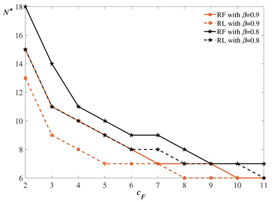
Figure 3. Optimal prescheduled preventive replacement times for unified models under each discipline, when $c_Y=0.4$.

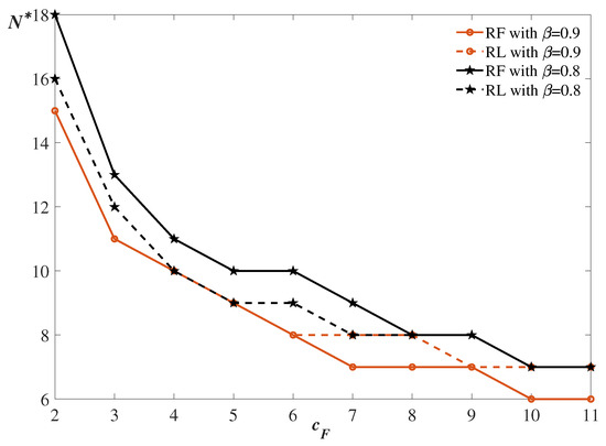
Figure 4. Optimal prescheduled preventive replacement times for unified models under each discipline, when $c_Y=1.0$.

(6)

The discounted factor cannot affect the structure of optimal preventive replacement policy, i.e., the above lessons (1)–(5) always hold with discounted factor $\beta =0.8$.

(7)

When the economic environment is more unstable, such as $\beta =0.8$, the optimal preventive replacement times $N^{*}$ will be delayed. When the economic environment is more unstable, for example, during times of economic uncertainty, the optimal timing for performing preventive equipment replacements will be postponed. This means that in uncertain economic conditions, people may delay replacing equipment or machinery to reduce costs or mitigate risks.

(8)

The associated expected costs $TC\left(N^{*}\right)$ under RF and RLdisciplines for each model have experienced a severe contraction in its overall size. We take Model 1 as an example. When $c_F=2.0$, $c_Y=0.4$, $\beta =0.9$, the optimal preventive replacement times $N^{*}$ and their associated expected costs $TC\left(N^{*}\right)$ are given by $N^{*}=15$, $T{C}_{f1}\left(N^{*}\right)=0.7585$ and $N^{*}=13$, $T{C}_{l1}\left(N^{*}\right)=0.7512$ in Table 1. When $c_F=2.0$, $c_Y=0.4$, $\beta =0.8$, the optimal preventive replacement times $N^{*}$ and their associated expected costs $TC\left(N^{*}\right)$ are given by $N^{*}=17$, $T{C}_{f1}\left(N^{*}\right)=0.2312$ and $N^{*}=15$, $T{C}_{l1}\left(N^{*}\right)=0.1868$ in Table 8.

7. Conclusions

In this paper, we have developed two opportunistic age replacement models in discrete time: the replacement first and replacement last models. We apply the NPV method to formulate the expected total costs. We have classified the cost model with discounting for each model into six cases by considering the priority of multiple replacement options. Some optimal opportunistic age replacement policies were discussed by optimizing the expected replacement costs over an infinite horizon. Also, we formulate a unified model under each discipline, merging six discrete time replacement models with probabilistic priority. In numerical illustration, we have presented a case study for pole air switches to obtain replacement policies for each discipline. The results indicate the following findings: (1) When the cost of the corrective replacement parameter significantly increases, the optimal prescheduled preventive replacement times $N^{*}$ reduce. The optimal prescheduled preventive replacement times $N^{*}$ also decrease with an increasing opportunistic cost parameter. (2) RL policy is only better than RF policy in some limited cases where the failure replacement cost $c_F$ is relatively small. (3) When the economic environment is more unstable, the optimal preventive replacement times $N^{*}$ will be delayed. The associated expected costs $TC\left(N^{*}\right)$ under RF and RL disciplines for each model have experienced a severe contraction in its overall size.

It is noted that there are some limitations in this paper:

(1)

Although we have found that RL policy is only better than RF policy in some limited cases where the failure replacement cost is relatively small, we cannot confirm that an RF policy with larger accurate cost parameter ranges equals an RL policy.

(2)

In our numerical illustrations, we simply applied the model parameters used by Wu et al. [4]. We aim to study other new discrete lifetime datasets from the manufacturing industry, such as the aerospace sector. We also aim to check the statistical properties of the discrete lifetime data.

(3)

We must acknowledge that although the experiments revealed several trends, real-world decision-making often demands a consideration of additional factors such as equipment significance, availability needs, and maintenance schedules. In addition, the discounted factor $\beta$ is not a constant value.

In future work, we will study the correlation between the life of the system and the arrival of replacement opportunity in an age-based replacement model. Dohi and Okamura [33] were first to recognize the significance of correlation between age and replacement opportunity and proposed opportunity-based models by introducing the bivariate copula with arbitrary marginal distributions, where they consider the correlation between age and the opportunity. So, we will further study the correlation between the life of the system and the arrival of replacement opportunity in discrete time models.

Appendix A.1. Derivation of Equation (1)

Here, we take the example of Model 1. According to the renewal function, we can obtain the NPV of the total expected cost over an infinite horizon.

$$\begin{array}{ccc}\hfill T{C}_{f1}\left(N\right)& =& \left[c_F+T{C}_{f1}\left(N\right)\right]\sum _{n=1}^{N-1}{\beta }^n{f}_Y\left(n\right)\overline{G}(n-1)+\left[c_Y+T{C}_{f1}\left(N\right)\right]\sum _{n=1}^{N-1}{\beta }^n{g}_X\left(n\right){\overline{F}}_Y\left(n\right)\hfill \\ & +& \left[c_T+T{C}_{f1}\left(N\right)\right]{\beta }^N{\overline{G}}_X(N-1){\overline{F}}_Y(N-1).\hfill \end{array}$$

(A1)

By a few algebraic manipulations, we can obtain

$$T{C}_{f1}\left(N\right)=\frac{C_{f1}\left(N\right)}{1-L_f\left(N\right)},$$

(A2)

where

$$L_f\left(N\right)=\sum _{n=1}^{N-1}{\beta }^n\left[f_Y\left(n\right)\overline{G}(n-1)+g_X\left(n\right){\overline{F}}_Y\left(n\right)\right]+{\beta }^N{\overline{G}}_X(N-1){\overline{F}}_Y(N-1),$$

(A3)

$$C_{f1}\left(N\right)=c_F\sum _{n=1}^{N-1}{\beta }^n{f}_Y\left(n\right)\overline{G}(n-1)+c_Y\sum _{n=1}^{N-1}{\beta }^n{g}_X\left(n\right){\overline{F}}_Y\left(n\right)+c_T{\beta }^N{\overline{G}}_X(N-1){\overline{F}}_Y(N-1).$$

(A4)

Appendix A.2. Monotonicity of Functions $w_{fj}(N\mid \beta )(j=1,\cdots ,6)$

Taking a further difference of $w_{fj}(N\mid \beta )$, we can obtain

$$\begin{array}{cc}\hfill w_{f1}(N+1\mid \beta )-w_{f1}(N\mid \beta )& =[\frac{\left(c_F-c_T\right)\left[{\Lambda }_Y(N+1)\left[1+{\Phi }_X(N+1)\right]-{\Lambda }_Y\left(N\right)\left[1+{\Phi }_X\left(N\right)\right]\right]}{1-\beta }\hfill \\ & -\frac{\left(c_T-c_Y\right)\left[{\Phi }_X(N+1)-{\Phi }_X\left(N\right)\right]}{1-\beta }]\left[1-L_f(N+1)\right],\hfill \end{array}$$

(A5)

$$\begin{array}{cc}\hfill w_{f2}(N+1\mid \beta )-w_{f2}(N\mid \beta )& =[\frac{\beta \left(c_F-c_T\right)\left[{\lambda }_Y(N+2)-{\lambda }_Y(N+1)\right]}{1-\beta }\hfill \\ & -\frac{\left(c_T-c_Y\right)\left[{\Phi }_X(N+1)-{\Phi }_X\left(N\right)\right]}{1-\beta }]\left[1-L_f(N+1)\right],\hfill \end{array}$$

(A6)

$$\begin{array}{cc}\hfill w_{f3}(N+1\mid \beta )-w_{f3}(N\mid \beta )& =[\frac{\left(c_F-c_T\right)\left[{\Lambda }_Y(N+1)-{\Lambda }_Y\left(N\right)\right]}{1-\beta }\hfill \\ & -\frac{\left(c_T-c_Y\right)\left[{\Phi }_X(N+1)\left[{\Lambda }_Y(N+1)+1\right]-{\Phi }_X\left(N\right)\left[{\Lambda }_Y\left(N\right)+1\right]\right]}{1-\beta }]\hfill \\ & \times \left[1-L_f(N+1)\right],\hfill \end{array}$$

(A7)

$$\begin{array}{cc}\hfill w_{f4}(N+1\mid \beta )-w_{f4}(N\mid \beta )& =[\frac{\left(c_F-c_T\right)\left[{\Lambda }_Y(N+1)-{\Lambda }_Y\left(N\right)\right]}{1-\beta }\hfill \\ & -\frac{\beta \left(c_T-c_Y\right)\left[{\varphi }_X(N+2)-{\varphi }_X(N+1)\right]}{1-\beta }]\hfill \\ & \times \left[1-L_f(N+1)\right],\hfill \end{array}$$

(A8)

$$\begin{array}{cc}\hfill w_{f5}(N+1\mid \beta )-w_{f5}(N\mid \beta )& =[\frac{\beta \left(c_F-c_T\right)\left[{\lambda }_Y(N+2)-{\lambda }_Y(N+1)\right]}{1-\beta }\hfill \\ & -\frac{\beta \left(c_T-c_Y\right)[{\varphi }_X(N+2)\left[1-{\lambda }_Y(N+2)\right]}{1-\beta }\hfill \\ & +\frac{{\varphi }_X(N+1)\left[1-{\lambda }_Y(N+1)\right]]}{1-\beta }]\left[1-L_f(N+1)\right],\hfill \end{array}$$

(A9)

$$\begin{array}{cc}\hfill w_{f6}(N+1\mid \beta )-w_{f6}(N\mid \beta )& =[\frac{\beta \left(c_F-c_T\right)[{\lambda }_Y(N+2)\left[1-{\varphi }_X(N+2)\right]}{1-\beta }\hfill \\ & -\frac{{\lambda }_Y(N+1)\left[1-{\varphi }_X(N+1)\right]]}{1-\beta }\hfill \\ & -\frac{\beta \left(c_T-c_Y\right)\left[{\varphi }_X(N+2)-{\varphi }_X(N+1)\right]}{1-\beta }]\hfill \\ & \times \left[1-L_f(N+1)\right].\hfill \end{array}$$

(A10)

From Equations (A5)–(A10), we can see that if the failure time Y strictly increases, then the arrival time of opportunity is a decreasing hazard function under Assumption 1. Then, additional necessary conditions of strictly $w_{fj}(N\mid \beta )$ are given in the following:

• Model 1: ${\Lambda }_Y(N+1){\Phi }_X(N+1)\ge {\Lambda }_Y\left(N\right){\Phi }_X\left(N\right)$;
• Model 2: None;
• Model 3: ${\Lambda }_Y(N+1){\Phi }_X(N+1)\le {\Lambda }_Y\left(N\right){\Phi }_X\left(N\right)$;
• Model 4: ${\lambda }_Y(N+1){\varphi }_X(N+1)\ge {\lambda }_Y\left(N\right){\varphi }_X\left(N\right)$;
• Model 5: None;
• Model 6: ${\lambda }_Y(N+1){\varphi }_X(N+1)\le {\lambda }_Y\left(N\right){\varphi }_X\left(N\right)$.

Appendix A.3. Proof for Theorem 1

Proof. 

Here, we only take the example of Model 1. Taking further difference of Equation (18) yields Equation (A5). When $w_{f1}(N+1\mid \beta )>w_{f1}(N\mid \beta )$, the function $T{C}_{f1}\left(N\right)$ is strictly convex in N. If $w_{f1}(N\mid \beta )>0$, then there exists at least one (at most two) optimal prescheduled preventive replacement time $N^{*}$, which satisfies $w_{f1}(N^{*}-1\mid \beta )<0$ and $w_{f1}(N^{*}\mid \beta )\ge 0$. Conversely, if $w_{f1}(N\mid \beta )\le 0$, then the function is monotonically decreasing. Then, the optimal prescheduled preventive replacement time is given by $N^{*}\to \infty$.

On the other hand, if $w_{f1}(N+1\mid \beta )\le w_{f1}(N\mid \beta )$, then the function $T{C}_{f1}\left(N\right)$ is concave in N for a fixed $\beta$. Thus, if $T{C}_{f1}\left(1\right)<T{C}_{f1}(\infty )$, then $N^{*}=1$, otherwise, $N^{*}\to \infty$. □

Appendix A.4. Monotonicity of Functions $w_{lj}(N\mid \beta )(j=1,\cdots ,6)$

Suppose that the failure time Y strictly increases under Assumption 1. Then, additional necessary conditions of strictly increasing $w_{lj}(N\mid \beta )(j=1,\cdots ,6)$ are given in the following:

• Model 1: $\left(c_F-c_T\right)\{{\Lambda }_Y\left(N\right){\Psi }_X\left(N\right)-{\Lambda }_Y(N+1){\Psi }_X(N+1)\}>\left(c_T-c_Y\right)\{{\Psi }_X\left(N\right)-{\Psi }_X$$(N+1)\}$;
• Models 2 and 5: $(c_F-c_T)\{{\lambda }_Y(N+2)-{\lambda }_Y(N+1)\}>(c_T-c_Y)\{{\Psi }_X\left(N\right)-{\Psi }_X(N+1)\}$;
• Models 3 and 4: $\{1+{\Lambda }_Y(N+1)\}{\Psi }_X(N+1)\ge \{1+{\Lambda }_Y\left(N\right)\}\Psi \left(N\right)$;
• Model 6: ${\Lambda }_Y(N+1){\Psi }_X(N+1)\ge {\Lambda }_Y\left(N\right){\Psi }_X\left(N\right)$; $\{1+{\Lambda }_Y(N+1)\}{\Psi }_X(N+1)\ge \{1+{\Lambda }_Y\left(N\right)\}{\Psi }_X\left(N\right)$.

References

- Zhao, X.; Nakagawa, T. Optimization problems of replacement first or last in reliability theory. Eur. J. Oper. Res. 2012, 223, 141–149. [Google Scholar] [CrossRef]
- Zhao, X.; Nakagawa, T.; Zuo, M.J. Optimal replacement last with continuous and discrete policies. IEEE Trans. Reliab. 2014, 63, 868–880. [Google Scholar] [CrossRef]
- Nakagawa, T. Advanced Reliability Models and Maintenance Policies; Springer: London, UK, 2008. [Google Scholar]
- Wu, J.; Qian, C.; Dohi, T. Optimal Opportunity-based Age Replacement Policies in Discrete Time. Reliab. Eng. Syst. Saf. 2024, 241, 109587. [Google Scholar] [CrossRef]
- Rander, R.; Jorgenson, D.W. Opportunistic replacement of a single part in the presence of several monitored parts. Manag. Sci. 1963, 10, 70–84. [Google Scholar]
- Berg, M. General trigger-off replacement procedures for two-unit systems. Nav. Res. Logist. 1978, 25, 15–29. [Google Scholar] [CrossRef]
- Dekker, R.; Dijkstra, M.C. Opportunity-based age replacement: Exponentially distributed times between opportunities. Nav. Res. Logist. 1992, 39, 175–190. [Google Scholar] [CrossRef][Green Version]
- Jhang, J.P.; Sheu, S.H. Opportunity-based age replacement policy with minimal repair. Reliab. Eng. Syst. Saf. 1999, 64, 339–344. [Google Scholar] [CrossRef]
- Dekker, R.; Smeitink, E. Preventive maintenance at opportunities of restricted duration. Nav. Res. Logist. 1994, 41, 335–353. [Google Scholar] [CrossRef]
- Dekker, R.; Smeitink, E. Opportunity-based block replacement. Eur. J. Oper. Res. 1991, 53, 46–63. [Google Scholar] [CrossRef][Green Version]
- Wang, J.; Miao, Y.; Yi, Y.; Huang, D. An imperfect age-based and condition-based opportunistic maintenance model for a two-unit series system. Comput. Ind. Eng. 2021, 160, 107583. [Google Scholar] [CrossRef]
- Si, G.; Xia, T.; Gebraeel, N.; Wang, D.; Pan, E.; Xi, L. A reliability-and-cost-based framework to optimize maintenance planning and diverse-skilled technician routing for geographically distributed systems. Reliab. Eng. Syst. Saf. 2022, 226, 108652. [Google Scholar] [CrossRef]
- Chen, M.; Zhao, X.; Nakagawa, T. Replacement policies with general model. Ann. Oper. Res. 2019, 277, 47–61. [Google Scholar] [CrossRef]
- Zhang, Q.; Xu, P.; Fang, Z. Optimal age replacement policies for parallel systems with mission durations. Comput. Ind. Eng. 2022, 169, 108172. [Google Scholar] [CrossRef]
- Cai, J.; Zhao, X. Optimal post-warranty replacement policies for batteries with mission durations. Ann. Oper. Res. 2022, 1–13. [Google Scholar] [CrossRef]
- Mizutani, S.; Zhao, X.; Nakagawa, T. Age and periodic replacement policies with two failure modes in general replacement models. Reliab. Eng. Syst. Saf. 2021, 214, 107754. [Google Scholar] [CrossRef]
- Sheu, S.H.; Liu, T.H.; Zhang, Z.G. Extended optimal preventive replacement policies with random working cycle. Reliab. Eng. Syst. Saf. 2019, 188, 398–415. [Google Scholar] [CrossRef]
- Nakagawa, T.; Osaki, S. Discrete time age replacement policies. J. Oper. Res. Soc. 1977, 28, 881–885. [Google Scholar] [CrossRef]
- Nakagawa, T. A summary of discrete replacement policies. Eur. J. Oper. Res. 1984, 17, 382–392. [Google Scholar] [CrossRef]
- Nakagawa, T. Optimal policy of continuous and discrete replacement with minimal repair at failure. Nav. Res. Logist. 1984, 31, 543–550. [Google Scholar] [CrossRef]
- Nakagawa, T. Continuous and discrete age-replacement policies. J. Oper. Res. Soc. 1985, 36, 147–154. [Google Scholar] [CrossRef]
- Cha, J.H.; Limnios, N. Discrete Time Minimal Repair Process and Its Reliability Applications under Random Environments. Stoch. Model. 2021, 1–22. [Google Scholar] [CrossRef]
- Eryilmaz, S. Revisiting discrete time age replacement policy for phase-type lifetime distributions. Eur. J. Oper. Res. 2021, 295, 699–704. [Google Scholar] [CrossRef]
- Eryilmaz, S. Age based preventive replacement policy for discrete time coherent systems with independent and identical components. Reliab. Eng. Syst. Saf. 2023, 240, 109544. [Google Scholar] [CrossRef]
- Wei, F.; Wang, J.; Ma, X.; Yang, L.; Qiu, Q. An Optimal Opportunistic Maintenance Planning Integrating Discrete-and Continuous-State Information. Mathematics 2023, 11, 3322. [Google Scholar] [CrossRef]
- Fox, B. Age replacement with discounting. Oper. Res. 1965, 14, 533–537. [Google Scholar] [CrossRef][Green Version]
- Nakagawa, T. A summary of block replacement policies. Rairo-Oper. Res. 1979, 13, 351–361. [Google Scholar] [CrossRef][Green Version]
- Chen, C.S.; Savits, T.H. A discounted cost relationship. J. Multivar. Anal. 1988, 27, 105–115. [Google Scholar] [CrossRef]
- van den Boomen, M.; Schoenmaker, R.; Wolfert, A.R.M. A life cycle costing approach for discounting in age and interval replacement optimisation models for civil infrastructure assets. Struct. Infrastruct. Eng. 2018, 14, 1–13. [Google Scholar] [CrossRef]
- Zhang, Q.; Yao, W.; Xu, P.; Fang, Z. Optimal age replacement policies of mission-oriented systems with discounting. Comput. Ind. Eng. 2023, 177, 109027. [Google Scholar] [CrossRef]
- Wu, J.; Qian, C.; Tadashi, D. Two Discrete-time Age-based Replacement Problems with/without Discounting. Int. J. Math. Eng. Manag. Sci. 2024, 9, 385–410. [Google Scholar] [CrossRef]
- Holland, C.; McLean, R.A. Applications of replacement theory. AIIE Trans. 1975, 7, 42–47. [Google Scholar] [CrossRef]
- Dohi, T.; Okamura, H. Failure-correlated opportunity-based age replacement models. Int. J. Reliab. Qual. Saf. Eng. 2020, 27, 2040008. [Google Scholar] [CrossRef]
Disclaimer/Publisher’s Note: The statements, opinions and data contained in all publications are solely those of the individual author(s) and contributor(s) and not of MDPI and/or the editor(s). MDPI and/or the editor(s) disclaim responsibility for any injury to people or property resulting from any ideas, methods, instructions or products referred to in the content. |
© 2024 by the authors. Licensee MDPI, Basel, Switzerland. This article is an open access article distributed under the terms and conditions of the Creative Commons Attribution (CC BY) license (https://creativecommons.org/licenses/by/4.0/).