Abstract
This article aims to introduce a set of hybrid matrix polynomials associated with -polynomials and explore their properties using a symbolic approach. The main outcomes of this study include the derivation of generating functions, series definitions, and differential equations for the newly introduced two-variable Hermite -matrix polynomials. Furthermore, we establish the quasi-monomiality property of these polynomials, derive summation formulae and integral representations, and examine the graphical representation and symmetric structure of their approximate zeros using computer-aided programs. Finally, this article concludes by introducing the idea of 1-variable Hermite matrix polynomials and their structure of zeros using a computer-aided program.
Keywords:
trigonometric functions; symbolic operator; hermite polynomials; λ-polynomials; distribution of zeros MSC:
33B10; 33F10; 33C65
1. Introduction
The field of orthogonal matrix polynomials is rapidly advancing, yielding significant results from both theoretical and practical perspectives. The role of Orthogonal matrices is advancing due to their essence in numerical computations, geometry, signal processing, coding theory, cryptography, and quantum mechanics. Their versatility and efficiency make them indispensable across various fields, driving ongoing research and development. Special functions, as a mathematical discipline, hold paramount significance for scientists and engineers across a myriad of application areas. The theory of special functions is highly significant in the formalism of mathematical physics. Hermite and Chebyshev polynomials, fully examined in the publication by [1,2], are fundamental special functions widely recognized for their broad range of applications in physics, engineering, and mathematical physics. These applications span from theoretical number theory to solving real-world problems in the disciplines of physics and engineering. In addition, the Hermite matrix polynomials have been introduced and thoroughly researched in several articles [3,4,5,6]. Matrix polynomials in special functions have a vital role in mathematical physics, electrodynamics, and image processing.
Multi-variable special polynomials hold significant importance across various mathematical domains and applications. Defined in multiple variables, they extend the principles of classical uni-variate polynomials into higher dimensions. These polynomials find utility in algebraic geometry, mathematical physics, and computer science. The exploration of multi-variable special polynomials encompasses diverse families, each characterized by unique properties and applications, establishing them as valuable tools for scholars and practitioners alike.
Hermite polynomials stand out as highly applicable orthogonal special functions dating back to the classical period. They serve as solutions to differential equations equivalent to the Schrödinger equation for a harmonic oscillator in quantum mechanics. Furthermore, these polynomials play a crucial role in the investigation of classical boundary-value problems in parabolic regions, particularly when utilizing parabolic coordinates.
Recently, it has been shown that the symbolic method provides a powerful and efficient means to introduce, study special functions, and reform special functions [7,8]. This method is also been proven to be helpful in introducing certain extensions of several special functions. The umbral formalism can be considered as a sub-field of the symbolic methods. In umbral formalism, we obtain suitable “umbra” based on some boundary conditions of the special polynomials.
Dattoli considered the idea of umbra denoted by , for 2VHKdFP as [9]:
where serve as the polynomial vacuum for 2VHKdFP thus, the action of yields 2VHKdFP .
The exponential of umbra is particularly important to derive the generating function for 2VHKdFP . In view of Equation (1), the exponential of umbra is of the form [9]:
In view of Equation (1), the umbral image of 2VHKdFP is given by
Recently, Dattoli et al. discovered a link between trigonometric functions and Laguerre polynomials. They proposed a way to introduce a new family of polynomials that connects Laguerre polynomials with trigonometric functions. This family of polynomials is known as -polynomials [10]. They expanded on this concept by adding a parameter and generalizing it to associated- polynomials.
The symbolic definition of associated- polynomials is of the form [10]:
where denotes a symbolic operator given by Dattoli et al. [11], which operates on the vacuum function as:
and
In particular, we have
The generating relation and explicit form of associated- polynomials are [10]:
and
respectively.
The associated cosine function is symbolically defined as [10]:
Recently, Zainab and Raza [12] introduced the 1-variable matrix polynomials by interchanging the role of u and v in the Equation (4) and then taking in the resultant expression as follows:
The symbolic image of polynomials is as follows [12]:
where matrix exponent of symbolic operator is given by
such that
where P and Q are positive stable matrices and .
The generating function and series definition of 1-variable matrix polynomials is given by [12]:
and
respectively.
The associated cosine matrix function is defined by means of the following symbolic images [12]:
The term “quasi-monomial” figures to the polynomial sequence , having two operators, especially named as multiplicative operator and derivative operator satisfying the following relations [13]:
and
respectively.
The following commutation relation satisfy by the operators and :
Thus, the operators and satisfy a weyl group structure [13]. By making use of the operators and , various characteristics of polynomial can be obtained. If and have differential realizations, then the following differential equation satisfies by the polynomial :
If represents the complex plane cut along the negative real axis, and denotes the principal logarithm of u, then is equivalent to . For a matrix P in , its two-norm, denoted by , is defined as , where for a vector represents the usual Euclidean norm, given by . The set containing all eigenvalues of P is denoted by . If and are holomorphic functions of the complex variable u, defined in an open set of the complex plane, and P is a matrix in such that , then the matrix functional calculus dictates that
If P is a matrix with , then denotes the image by The matrix functional calculus acts on the matrix P. We say that P is a positive stable matrix [4,5,14] if
In this paper, we propose a convolution between the two variables Hermite polynomials and the -matrix polynomials to introduce a new family of polynomials called the 2-variable Hermite -matrix polynomials. Section 2 delves into this newly introduced family’s generating function, series definition, differential equation, and differential recurrence relation. Also, we establish the quasi-monomiality property of these polynomials. In Section 3, we obtain some summation formulae. In Section 4, by using the computer-aided program (Wolfram Mathematica), we consider some examples of this hybrid family and give their graphical representations, mainly to observe from several angles how zeros of these polynomials are distributed and located. Section 5 concludes this paper by introducing the concept of 1-variable Hermite -matrix polynomials and obtaining their zeros.
2. Hermite -Matrix Polynomials
In this section, we introduce the 2-variable Hermite -matrix polynomials by using a symbolic approach and obtain their generating function, series definition, multiplicative and derivative operators, differential equation, and differential recurrence relation.
Now, we recall the generating function and series definition of Classical Hermite polynomials . The classical Hermite polynomials are defined by the means of the following generating function [1]:
and explicit representation
respectively.
2-variable Hermite Kempe de Fériet polynomials (2VHKdFP) is given by the following generating relation and series definition [15]:
and
respectively.
Now, we introduce the 2-variable Hermite -matrix polynomials (2vHMP) by replacing u in (11) with the symbolic operator of Hermite polynomial as
We obtain the following theorem for generating function and series definition of Hermite -matrix polynomials :
Theorem 1.
The following generating function and series definition hold true for Hermite λ-matrix polynomials :
and
respectively.
Proof.
Since, ,
Again from the Equation (27), we get
In view of Equation (3), we get
In view of Equation (6), we get
Theorem 2.
The Hermite λ-matrix polynomials are quasi-monomial with respect to the following multiplicative and derivative operators:
and
respectively.
Proof.
Operating on both sides of Equation (27), we get
which on again using Equation (27), gives
again in view of Equations (17) and (39) we have the assertion (36).
Theorem 3.
The differential equation satisfied by Hermite λ-matrix polynomial is given by
Theorem 4.
The Hermite λ-matrix polynomials satisfy the following differential reccurence relation:
More generally,
Proof.
On differentiating Equation (28) with respect to u, we have
which in view of Equation (28), we have
or, equivalently
On comparing the equal powers of s, we get the assertion (43).
3. Summation Formulae
In this section, we obtain certain summation formulae for 2vHMP :
Theorem 5.
The following summation formula for Hermite λ- matrix polynomials holds true:
Proof.
Or, equivalently
Expanding the second exponential in the right-hand side of the above equation and using Equation (31) in the resultant equation, we have
which on using the following series rearrangement
in the right hand side of Equation (51), we have
Comparing the equal powers of s from both sides of the above equation, we get the assertion (48). □
We obtain the following another theorem for summation formulae for Hermite - matrix polynomial :
Theorem 6.
The following summation formula for Hermite λ- matrix polynomial holds true:
where .
Proof.
Replacing s by in the Equation (31) and then using the formula [16]:
in the right-hand side of the resultant equation, we find the following generating function for Hermite - matrix polynomial :
which can be written as
4. Graphical Representation and Distribution of Zeros
In this section, we obtain certain examples and give their graphical representation and distribution of zeros of 2-variable Hermite -matrix polynomials.
Example 1.
Example 2.
Since in view of Equations (4) and (11), for , the λ-matrix polynomials transform to the associated-λ polynomials . Therefore, for the same choice of P, 2vHλMP transform to 2-variable Hermite λ associated polynomials (2vHaλP) . Thus, for Equations (27)–(29), (36), (37) and (42)–(44) reduce to respective symbolic definition, generating function, series definition, multiplicative operator, derivative operator, differential equation and differential recurrence relation for 2vHaλP .
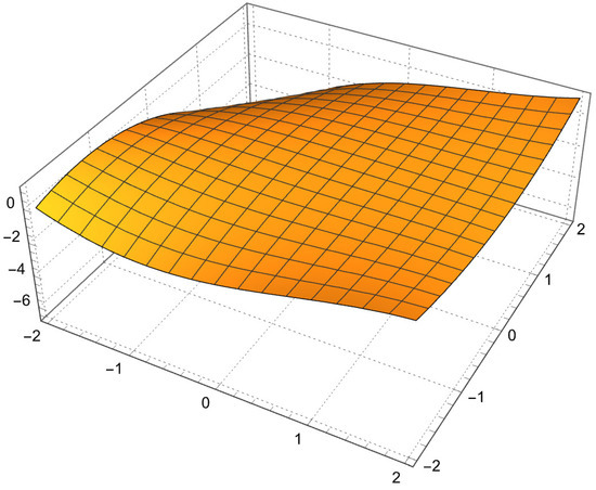
Figure 1.
Surface plot of .
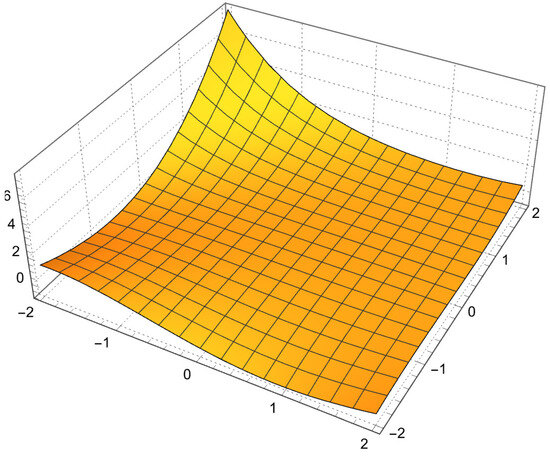
Figure 2.
Surface plot of .
Now, we find the roots of equation for different choices for v. Figure 3 shows the roots of the equation , Figure 4 shows the roots of the equation , whereas Figure 5 and Figure 6 show the roots of the equation and , respectively. Certain roots of the equation and beautiful graphical representation are shown. We plot the zeros of the 2vHaP for and different choices of v and in Figure 3, Figure 4, Figure 5 and Figure 6. Some recent developments in this field can be found in [17,18].
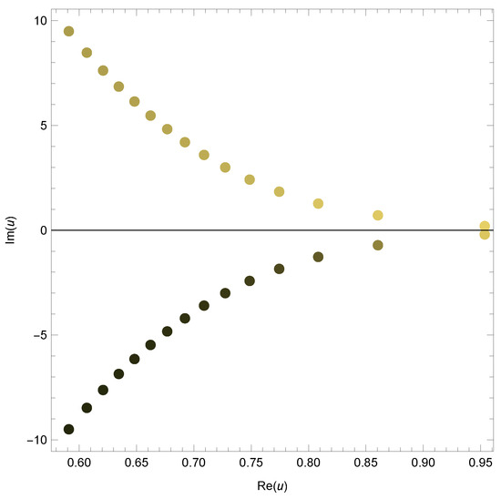
Figure 3.
Zeros of 2vHaP .
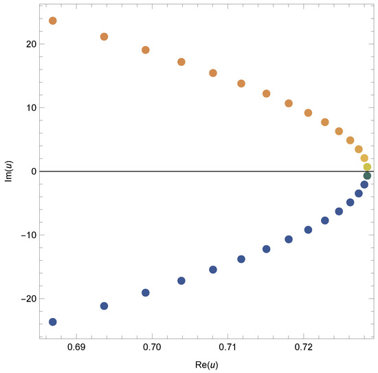
Figure 4.
Zeros of 2vHaP .
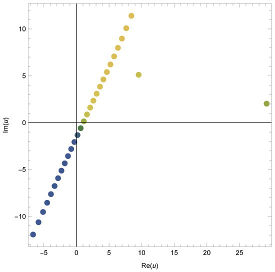
Figure 5.
Zeros of 2vHaP .
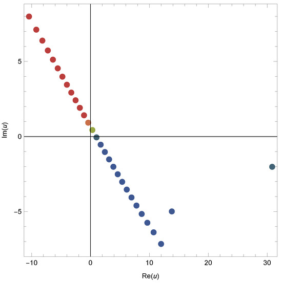
Figure 6.
Zeros of 2vHaP .
In Figure 3, we choose and . In Figure 4, we choose and . In Figure 5, we choose and In Figure 6, we choose and .
Plots of real roots of the 2vHaP for are presented in Figure 7 and Figure 8. In Figure 7, we choose and . In Figure 8, we choose and . It is worth noticing that for negative values of v, no of real roots are more than that of positive values of v. Stacks of roots of the 2vHaP for , and from a 3D structure are presented in Figure 9.
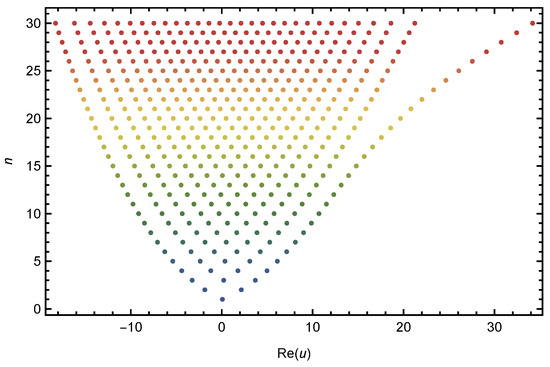
Figure 7.
Real zeros of .
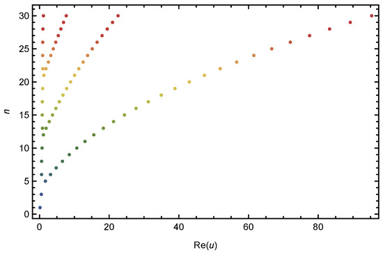
Figure 8.
Real zeros of .
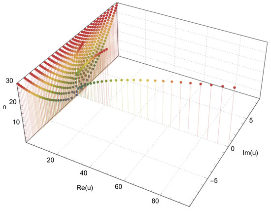
Figure 9.
Stacks of zeros of .
Our numerical results for the solutions satisfying 2vHaP for and are listed in Table 1.

Table 1.
Approximate solutions of 2vHaP .
5. Concluding Remarks
In concluding remarks, we introduce the idea of 1-variable Hermite -matrix polynomials (1vHMP) .
From Equations (23) and (25) it is clear that the 2VHKdFP is related to the classical Hermite polynomials as:
Similarly, taking into account Equation (63), we obtain the generating function and series definition of 1vHMP :
and
respectively.
The multiplicative and derivative operators of 1vHMP :
and
respectively.
In view of Equations (20), (66) and (67), the following differential equation is satisfied by 1vHMP :
Since in view of Equations (4) and (11), for , the -matrix polynomials transform to the associated- polynomials . Therefore, for the same choice of P, 1vHMP transform to 1-variable Hermite associated associated polynomials (1vHaP) . Thus, for Equations (63)–(68) reduce to respective symbolic definition, generating function, series definition, multiplicative operator, derivative operator, and differential equation for 1vHaP .
Now, we illustrate the shape of 1vHaP and examine its zeros. In Figure 10, we present the graphs of 1vHaP .
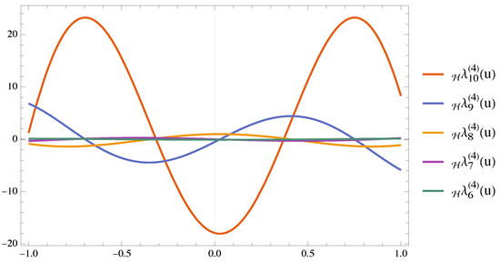
Figure 10.
.
Our numerical results for the solutions satisfying 1vHaP for and are listed in Table 2.
Table 2.
Approximate solutions of 1vHaP .
Next in Figure 11 and Figure 12, we investigate the beautiful pattern of zeros of the 1vHaP . The plot of real zeros of the 1vHaP for for structure are presented in Figure 11.
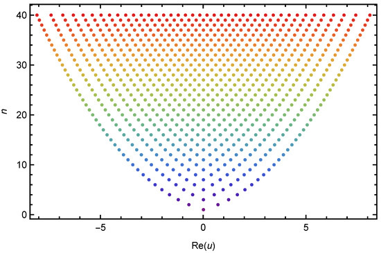
Figure 11.
Real zeros of .
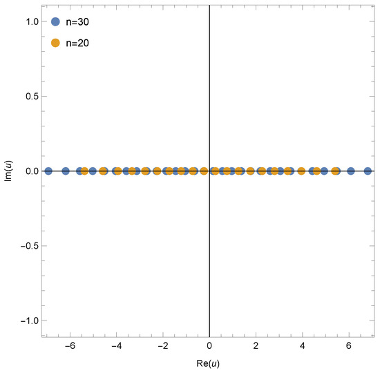
Figure 12.
Zeros of .
We can discern a consistent pattern in the complex roots of the 2-variable Hermite associated polynomials . Consequently, the following conjectures are plausible for the equation 1vHa.
We observed that the solutions of the 1vHaP equations exhibit no reflection symmetry for . It is anticipated that the solutions of the 1vHa equations possess reflection symmetry (refer to Figure 11 and Figure 12).
Conjecture 1.
Prove or disprove that 1vHaλP for and has reflection symmetry analytic complex functions.
Finally, we addressed the more general problem of determining the number of zeros of the equation . We were unable to ascertain whether this equation has n distinct solutions. Our interest lies in determining the number of complex zeros of the equation .
Conjecture 2.
Prove or disprove that 1vHaλP have n distinct roots.
As a result of investigating more n variables, it is still unknown whether the above conjectures are true or false for all variables n.
In this article, our aim is to introduce the set of hybrid matrix polynomials associated with -polynomials and explore their properties using a symbolic approach. The main outcomes of this study include the derivation of generating functions, series definitions, and differential equations for the newly introduced two-variable Hermite -matrix polynomials. Furthermore, we establish the quasi-monomiality property of these polynomials and derive summation formulae. Finally, we obtain the graphical representation and symmetric structure of their approximate zeros for different choices of , and using computer-aided programs.
The results of this article have the potential to motivate researchers and readers to conduct further research on these special matrix polynomials. These results may be applied in mathematics, mathematical physics, and engineering.
Author Contributions
Conceptualization, M.S.A., M.K., N.R. and W.A.K.; methodology, M.S.A., M.K., N.R. and W.A.K.; software, M.K. and N.R.; validation, M.S.A., M.K., N.R. and W.A.K.; formal analysis, M.S.A., M.K., N.R. and W.A.K.; investigation, M.K. and N.R.; writing—original draft preparation, M.K. and N.R.; writing—review and editing, M.S.A., M.K., N.R. and W.A.K.; project administration, M.S.A., M.K., N.R. and W.A.K.; funding acquisition, M.S.A. All authors have read and agreed to the published version of the manuscript.
Funding
This research received no external funding.
Data Availability Statement
No data were used to support this study.
Conflicts of Interest
The authors declare no conflicts of interest.
References
- Rainville, E.D. Special Functions; Macmillan: New York, NY, USA, 1960. [Google Scholar]
- Rainville, E.D. Special Functions; Macmillan; Chelsea Publ. Co.: Bronx, NY, USA, 1971. [Google Scholar]
- Batahan, R.S. A new extension of Hermite matrix polynomials and its applications. Linear Algebra Appl. 2006, 419, 82–92. [Google Scholar] [CrossRef][Green Version]
- Jódar, L.; Defez, E. On Hermite matrix polynomials and Hermite matrix functions. J. Approx. Theory Appl. 1998, 14, 36–48. [Google Scholar] [CrossRef]
- Metwally, M.S.; Mohamed, M.T.; Shehata, A. On Hermite-Hermite matrix polynomials. Math. Bohem. 2008, 133, 421–434. [Google Scholar] [CrossRef]
- Sayyed, K.A.M.; Metwally, M.S.; Batahan, R.S. On generalized Hermite matrix polynomials. Electron. J. Linear Algebra 2003, 10, 272–279. [Google Scholar] [CrossRef][Green Version]
- Dattoli, G.; Germano, B.; Licciardi, S.; Martinelli, M.R. On an umbral treatment of Gegenbauer, Legendre and Jacobi polynomials. Int. Math. Forum 2017, 12, 531–551. [Google Scholar] [CrossRef]
- Dattoli, G.; Licciardi, S. Operational, umbral methods, Borel transform and negative derivative operator techniques. Integral Transform. Spec. Funct. 2020, 31, 192–220. [Google Scholar] [CrossRef]
- Dattoli, G.; Germano, B.; Martinelli, M.R.; Ricci, P.E. Lacunary generating functions of Hermite polynomials and symbolic methods. Ilir. J. Math. 2015, 4, 16–23. [Google Scholar]
- Dattoli, G.; Licciardi, S.; Palma, E.D.; Sabia, E. From circular to Bessel functions: A transition through the umbral method. Fractal Fract. 2017, 1, 9. [Google Scholar] [CrossRef]
- Dattoli, G.; Gorska, K.; Horzela, A.; Licciardi, S.; Pidatella, R.M. Comments on the properties of Mittag-Leffler function. Eur. Phys. J. Spec. Top. 2017, 226, 3427–3443. [Google Scholar] [CrossRef]
- Zainab, U.; Raza, N. The symbolic approach to study the family of Appell- λ matrix polynomials. Filomat 2024, 38, 1291–1304. [Google Scholar]
- Dattoli, G. Hermite-Bessel and Laguerre-Bessel functions: A by-product of the monomiality principle. Adv. Spec. Funct. Appl. 1999, 1, 147–164. [Google Scholar]
- Defez, E.; Hervás, A.; Jódar, L.A. Law: Bounding Hermite matrix polynomials. Math. Computer Model. 2004, 40, 117–125. [Google Scholar] [CrossRef]
- Appell, P.; Kampé de Fériet, J. Fonctions Hypergéométriques et Hypersphériques: Polynômes d’Hermite; Gautier Villars: Paris, France, 1926. [Google Scholar]
- Srivastava, H.M.; Manocha, H.L. A Treatise on Generating Functions; Hasted Press-Ellis Horwood Limited-John Wiley and Sons: New York, NY, USA; Chichester, UK; Brisbane, Australia; Toronto, ON, Canada, 1984. [Google Scholar]
- Al e’damat, A.; Khan, W.A.; Duran, U.; Kirmani, S.A.K.; Ryoo, C.-S. Exploring the depths of degenerate hyper-harmonic numbers in view of harmonic functions. J. Math. Comput. Sci. 2024, 35, 136–148. [Google Scholar] [CrossRef]
- Alatawi, M.S.; Khan, W.A.; Kızılateş, C.; Ryoo, C.S. Some Properties of Generalized Apostol-Type Frobenius–Euler–Fibonacci Polynomials. Mathematics 2024, 12, 800. [Google Scholar] [CrossRef]


Disclaimer/Publisher’s Note: The statements, opinions and data contained in all publications are solely those of the individual author(s) and contributor(s) and not of MDPI and/or the editor(s). MDPI and/or the editor(s) disclaim responsibility for any injury to people or property resulting from any ideas, methods, instructions or products referred to in the content. |
© 2024 by the authors. Licensee MDPI, Basel, Switzerland. This article is an open access article distributed under the terms and conditions of the Creative Commons Attribution (CC BY) license (https://creativecommons.org/licenses/by/4.0/).