Source Design Optimization for Depth Image Reconstruction in X-ray Imaging

Abstract

X-ray tomography is an effective non-destructive testing method for industrial quality control. Limited-angle tomography can be used to reduce the amount of data that need to be acquired and thereby speed up the process. In some industrial applications, however, objects are flat and layered, and laminography is preferred. It can deliver 2D images of the structure of a layered object at a particular depth from very limited data. An image at a particular depth is obtained by summing those parts of the data that contribute to that slice. This produces a sharp image of that slice while superimposing a blurred version of structures present at other depths. In this paper, we investigate an Optimal Experimental Design (OED) problem for laminography that aims to determine the optimal source positions. Not only can this be used to mitigate imaging artifacts, it can also speed up the acquisition process in cases where moving the source and detector is time-consuming (e.g., in robotic arm imaging systems). We investigate the imaging artifacts in detail through a modified Fourier Slice Theorem. We address the experimental design problem within the Bayesian risk framework using empirical Bayes risk minimization. Finally, we present numerical experiments on simulated data.

1. Introduction

Non-destructive testing is essential in industrial quality control [1]. X-ray imaging in particular is a highly effective non-destructive testing technique that can deliver detailed 3D images of the internal structure of products. It is widely employed across various industries for quality control [2,3]. Conventional tomographic acquisition requires a full rotation around the object, limiting its applicability to the off-line inspection of small-to-medium-sized objects. To overcome this limitation, several approaches to tomographic reconstruction from limited-angle data have been developed. These methods often rely on additional prior knowledge of the object to fill in information that is missing in the measurements. A prime example is discrete tomography, where objects consisting of a few distinct materials can be reconstructed from severely under-sampled data. In certain applications where objects are wide and flat, tomographic data can only be collected over a very limited angular range. This pushes the limits of conventional limited-angle tomography and we have to resort to another class of methods [4]. Laminography offers a method to reconstruct an image of a specific slice of a flat layered object. As shown in Figure 1, it needs a flexible source and detector that can move and collect data from several directions such that during scanning the X-ray tube is located on the same side of the flat object and the detector is on the opposite side of it [5].

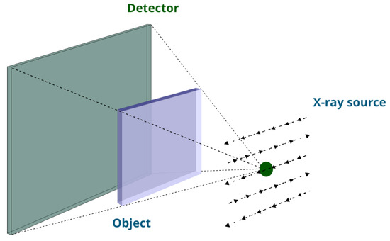
Figure 1. A laminographic setup designed for scanning flat objects, featuring a flexible source that moves along a raster trajectory. Note that dashed arrows specify the source trajectory.

In this paper, we consider a particular setup for laminographic imaging which requires the acquisition of X-ray projection images from N source positions on a fixed grid, while the detector is fixed on the opposite side of the object. Our aim is to be able to optimally design acquisition protocols with $K\le N$ sources for a given set of objects. By optimally designing the setup, we can reduce imaging artifacts as well as potentially speed up the data acquisition process, particularly in scenarios where adjusting the source position is time-consuming, such as in robotic arm imaging systems. Bayesian Optimal Experimental Design (OED) is a mathematical approach that facilitates the design of experimental parameters while minimizing experimental costs. It utilizes prior knowledge and Bayesian inference to refine the selection of experimental settings, thereby improving data collection efficiency and decision-making effectiveness [6]. Various criteria, including D-optimality and A-optimality, are frequently employed to assess and compare the efficacy of experimental designs [6,7]. D-optimality focuses on maximizing the Kullback–Leibler divergence between the posterior and prior distributions, whereas A-optimality aims to minimize the expected error between reconstructions and actual ground truths [8,9]. In [10], the authors proposed the optimization of projection angles in X-ray imaging. They incorporated empirical A-optimal design in constrained problems based on calibration data. Specifically, they obtained a sparse design out of a predetermined set of angles and implemented it with a gradient-based optimization method. Similarly, we pose the OED problem for laminography as a bilevel optimization based on the A-optimality criterion. Additionally, we employ gradient-based methods to facilitate implementation in high-dimensional settings.

Our main contributions are the following:

• We analyze the 3D and 2D (slice-based) image reconstruction process for laminography, present an analog of the Fourier Slice Theorem specific to this setup, and analyze the image artifacts present in slice images.
• We pose an experimental design problem for selecting the K most informative source positions for laminography across a specific class of objects. Additionally, we formulate a bilevel optimization within the Bayes risk minimization framework to solve it.

The remainder of this paper is organized as follows: In Section 2, we present the forward and backward operators in the continuous domain for the depth imaging procedure. We study depth reconstruction in the discrete domain in Section 3. In Section 4, we propose a bilevel optimization problem to find a source design with K sources chosen from a fixed array of $N\ge K$ sources. In Section 5, we propose an algorithm to solve the proposed bilevel optimization problem and present its pseudocode in Section 6. In Section 7, we show the results obtained by our method and compare them to optimal source designs obtained by exhaustive search. Finally, Section 8 and Section 9 discuss the limitations and future directions of our research and conclude the paper, respectively.

Notation

Throughout this paper, scalars and vector elements are denoted by lower-case letters, vectors by lower-case boldface letters, and matrices by upper-case boldface letters. The notation ${·}^{\top }$ stands for a transpose of either a vector or matrix. Moreover, # denotes the cardinality of a vector and $\parallel \mathit{x}\parallel =\sqrt{{\sum }_{i=1}^n{x}_i^2}$ denotes the ${\mathsf{\ell }}_2$ norm of a vector.

2. Forward and Backward Operators in the Continuous Domain

In this section, we first review the linear X-ray projection model. Subsequently, we introduce the forward and backward operators as depicted in Figure 2. Finally, we detail the depth imaging process for laminography in the continuous domain, utilizing these operators.

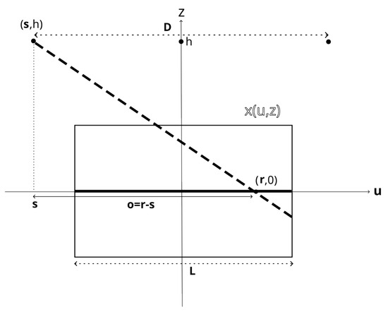
Figure 2. Two-dimensional view of the acquisition setup. The source is located at lateral position $\mathit{s}\in {\mathbb{R}}^2$ and height h; the detector is parameterized without loss of generality by $\mathit{r}\in {\mathbb{R}}^2$. The object is characterized by x as a function of lateral coordinate $\mathit{u}$ and vertical coordinate z. The ray from the source to the detector is shown by the dashed line.

Briefly, the forward projection operator transforms the object’s internal features into the collected projection data, effectively modeling the imaging process. Conversely, the backward projection operator transforms the projection data back into a representation of the object’s internal features, serving as the basis for reconstructing the original image [11].

2.1. Linear Projection Model

During the X-ray imaging process, an object is exposed to a beam of X-ray photons emitted by an X-ray tube. Some of these photons are absorbed by the object, while others reach the detector. The captured measurements can be modeled using the Beer–Lambert law, which describes the exponential relationship between the intensity of the X-ray beam and the distance it travels through the object:

$$\begin{array}{c}\hfill I_i=I_{0}exp\left(-\int x\left({\mathit{t}}_i+{\mathit{\eta }}_{i}r\right)\mathrm{d}r\right),\end{array}$$

(1)

where $I_i$ denotes the number of photons that reach the detector from starting point ${\mathit{t}}_i$ in the direction of ${\mathit{\eta }}_i$, where $i=1,\dots ,m$. $I_0$ is the initial intensity of the beam (i.e., the number of photons emitted by the source), and x is the function representing the attenuation coefficient of the object. This relation is usually written as

$$\begin{array}{c}\hfill y_i=\int x\left({\mathit{t}}_i+{\mathit{\eta }}_{i}r\right)\mathrm{d}r,\end{array}$$

(2)

with $y_i=-log\frac{I_i}{I_0}$ representing the measured data for a single ray. In the following, we present the forward and backward operators for the X-ray setup shown in Figure 2. To study the depth imaging procedure within this specific setup, we need to understand forward and backward operators for both 2D and 3D objects.

2.2. Forward and Backward Operators for the Slice Imaging Setup

The proposed imaging setup is schematically depicted in Figure 2. X-rays are emitted by a source at lateral position $\mathit{s}\in {\mathbb{R}}^2$ and height h. Without loss of generality, we parameterise the detector position by $\mathit{r}\in {\mathbb{R}}^2$. The forward operator, $\mathcal{A}$, is now given by

$$y(\mathit{r},\mathit{s})=\left(\mathcal{A}x\right)(\mathit{r},\mathit{s})=\int x\left(t\mathit{r}+(1-t)\mathit{s},(1-t)h\right)\mathrm{d}t,$$

(3)

as shown in Figure 2. Here, $x(\mathit{u},z)$ denotes the attenuation coefficient of the object in terms of its lateral ($\mathit{u}\in {\mathbb{R}}^2$) and vertical ($z\in \mathbb{R}$) coordinates. In fact, it integrates along the ray from the source at $(\mathit{s},h)$ to the detector located at $(\mathit{r},0)$.

2.2.1. The Fourier Slice Theorem

The Fourier Slice Theorem illustrates the relationship between the collected measurements and the Fourier transform of the object. In traditional computed tomography, a complete sampling process enables the straightforward inversion of the Radon transform using the filtered back projection method [12]. Due to the limited acquisition view in laminography, the Fourier Slice Theorem shows that some parts of the object spectrum are missing. The absence of complete data leads to the appearance of artifacts within the reconstructed image at specific depths. According to the setup shown in Figure 2, we define the measurements in receiver-offset coordinates as $g(\mathit{r},\mathit{o})=y(\mathit{r},\mathit{r}-\mathit{o})$ and find the following relation between the 2D Fourier transform of g and the 3D Fourier transform of x. Let $\mathit{\xi }$ and $\zeta$ represent the spatial frequency coordinates. Then, it reads as follows (see the derivation in Appendix A.2):

$$\begin{array}{cc}\hfill {\mathcal{F}}_{2D}\left(g\right)(\mathit{\xi },\mathit{o})& ={\mathcal{F}}_{3D}\left(x\right)(\mathit{\xi },\zeta ),\hfill \\ \hfill \zeta & =h^{-1}{\mathit{\xi }}^{\top }\mathit{o},\hfill \end{array}$$

(4)

where ${\mathcal{F}}_{2D}$ and ${\mathcal{F}}_{3D}$ denote the 2D and 3D Fourier transforms, respectively, and $\mathit{o}=\mathit{r}-\mathit{s}$ signifies the vector difference between the detector position $\mathit{r}$ and the source position $\mathit{s}$. Figure 3 depicts sampled elements ${\mathcal{F}}_{2D}\left(g\right)$ (black circles) with respect to the Fourier object samples ${\mathcal{F}}_{3D}\left(x\right)$ (shown by green squares). Obviously, the sampling procedure is missing a portion of the object spectrum due to the limited values of $\mathit{o}$, i.e., the forward operator samples from $\zeta =h^{-1}{\mathit{\xi }}^{\top }\mathit{o}$. Since the range of $\mathit{o}$ is finite, this leads to a missing wedge in the frequency domain. This missing wedge leads to an ill-posed inverse problem of recovering x from g (or, equivalently, y).

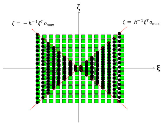
Figure 3. Schematic depiction of the missing wedge in the Fourier domain sampling of ${\mathcal{F}}_{3D}\left(x\right)$ by the measurements ${\mathcal{F}}_{2D}\left(g\right)$. The green squares represent ${\mathcal{F}}_{3D}\left(x\right)\left(\mathit{\xi },\zeta \right)$ and black circles represent ${\mathcal{F}}_{2D}\left(g\right)\left(\mathit{\xi },\mathit{o}\right)$, which are limited in $\zeta$ by $h^{-1}{\mathit{\xi }}^{\top }{\mathit{o}}_{max}$. The limited aperture in $\mathit{o}$ gives rise to the missing wedge.

2.2.2. The 2D Slice at Depth z

To study the depth imaging procedure, we introduce the corresponding forward operator ${\mathcal{A}}_z$ which maps a 2D image at depth z, denoted by $x_z\left(\mathit{u}\right)$, to the corresponding projection data $y(\mathit{r},\mathit{s})$ (see Appendix A.3):

$$\begin{array}{c}\hfill y\left(\mathit{r},\mathit{s}\right)=\left({\mathcal{A}}_z{x}_z\right)(\mathit{s},\mathit{r})=x_z\left(\left(1-h^{-1}z\right)\mathit{r}+h^{-1}z\mathit{s}\right),\end{array}$$

(5)

the corresponding adjoint operator ${\mathcal{A}}_z^{\ast }$ is given by (see Appendix A.3):

$$\begin{array}{c}\hfill \left({\mathcal{A}}_z^{\ast }y\right)\left(\mathit{u}\right)=\frac{1}{1-h^{-1}z}\int y\left(\frac{\mathit{u}-h^{-1}z\mathit{s}}{1-h^{-1}z},\mathit{s}\right)\mathrm{d}\mathit{s},\end{array}$$

(6)

we then find that ${\mathcal{A}}_z^{\ast }{\mathcal{A}}_z$ is given by

$$\begin{array}{c}\hfill \left({\mathcal{A}}_z^{\ast }{\mathcal{A}}_z{x}_z\right)\left(\mathit{u}\right)=\frac{\int \mathrm{d}\mathit{s}}{1-h^{-1}z}{x}_z\left(\mathit{u}\right),\end{array}$$

(7)

so that for a limited range of $\mathit{s}$, ${\mathcal{A}}_z^{\ast }{\mathcal{A}}_z\propto \mathcal{I}$ and hence is trivially inverted. Depth imaging of an object consisting of a single thin layer can thus be achieved by a simple back projection. When multiple layers are present we expect artifacts, which we study next.

2.3. Depth Image Reconstruction

Here, we are interested in studying the artifacts that arise when imaging a slice from measurements of a 3D layered object. In the remainder of this section, we let $h=1$ for ease of notation. As argued above, we can form a depth image by back projection, so it suffices to study the operator ${\mathcal{A}}_z^{\ast }\mathcal{A}$ (see Appendix A.4). In particular, we expect to image layered objects, which we can model as

$$x(\mathit{u},z)=\sum _{i=1}^M{x}_i\left(\mathit{u}\right)\delta (z-z_i),$$

using a finite number of sources ${\left\{{\mathit{s}}_j\right\}}_{j=1}^N$, the depth image of the $k^{\mathrm{th}}$ layer is then given by

$$\begin{array}{cc}\hfill {\tilde{x}}_k\left(\mathit{u}\right)& =\sum _{i=1}^M\sum _{j=1}^N{x}_i\left(\frac{1-z_i}{1-z_k}\mathit{u}+\frac{z_i-z_k}{1-z_k}{\mathit{s}}_j\right)\hfill \end{array}$$

(8)

$$\begin{array}{cc}\hfill & \hfill =x_k\left(\mathit{u}\right)+N^{-1}\sum _{i\ne k}\sum _{j=1}^N{x}_i\left(\frac{1-z_i}{1-z_k}\mathit{u}+\frac{z_i-z_k}{1-z_k}{\mathit{s}}_j\right)\end{array}$$

(9)

Hence, the error in the depth image of the $k^{\mathrm{th}}$ layer is a superposition of spatially averaged versions of the other layers. An illustration of the resulting spatial sampling patterns is shown in Figure 4.

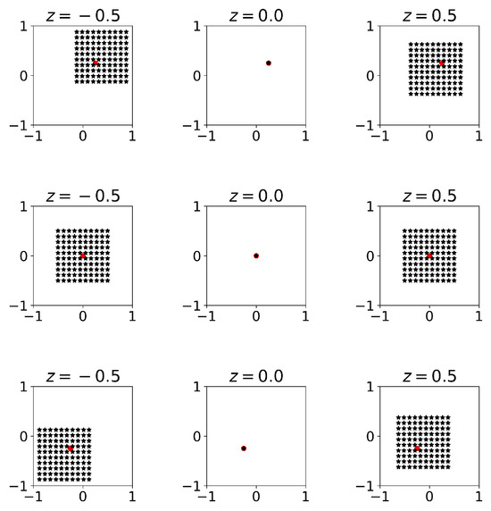
Figure 4. Example of the spatial sampling patterns when imaging the middle layer (at $z=0$ ) of an object with $M=3$ layers and $N=100$ regularly spaced sources in ${[-1,1]}^2$ at $z=1$. The red circle indicates the point $\mathit{u}$ at which we evaluate the output.

So far, it is evident that imaging a specific depth of a flat object leads to artifacts, as demonstrated by the derived depth image in Equation (9). Furthermore, these artifacts are influenced by the positions of the X-ray sources. The source design problem is now to identify a configuration of source positions, ${\mathit{s}}_j$, that minimize unwanted features in the depth image. As we do not expect to be able to find a closed-form solution to the source design problem in general, we discretize the problem and resort to numerical optimization.

3. Discrete Problem

In this section, we explore depth imaging in the discrete domain, discuss the challenges that arise from it, and present the algebraic reconstruction technique for addressing these challenges.

3.1. Forward and Back Projection

We discretize the forward model in (3) and express it as

$$\begin{array}{c}\hfill \mathit{y}=\mathit{A}\mathit{x},\end{array}$$

(10)

where $\mathit{y}\in {\mathbb{R}}^m$, $\mathit{x}\in {\mathbb{R}}^n$, and $\mathit{A}\in {\mathbb{R}}^{m\times n}$. Note that the number of rows in $\mathit{A}$ is the product of the number of detector pixels and the number of sources. Every block of rows corresponds to a particular X-ray source.

Let ${\mathit{A}}_z$ and ${\mathit{x}}_z$ denote the forward matrix and the slice object at depth z, respectively. In general, ${\mathit{A}}_z^{\top }{\mathit{A}}_z$ will not be a multiple of the identity as in the continuous setting (7), so we consider solving ${\mathit{A}}_z^{\top }{\mathit{A}}_z{\mathit{x}}_z={\mathit{A}}_z^{\top }\mathit{y}$. We can view this as an approximation of 3D reconstruction through the Schur complement [13]. To see this, let ${\mathit{A}}_c$ and ${\mathit{x}}_c$ represent the forward operator and the object for all pixels except the ones contained in ${\mathit{x}}_z$. The linear equations for the forward projection (10) can now be expressed as follows:

$$\begin{array}{c}\hfill \left[\begin{array}{cc}{\mathit{A}}_z& {\mathit{A}}_c\end{array}\right]\left[\begin{array}{c}{\mathit{x}}_z\\ {\mathit{x}}_c\end{array}\right]=\mathit{y}.\end{array}$$

(11)

By multiplying ${\mathit{A}}^{\top }$, it reads

$$\begin{array}{c}\hfill \left[\begin{array}{cc}{\mathit{A}}_z^{\top }{\mathit{A}}_z& {\mathit{A}}_z^{\top }{\mathit{A}}_c\\ {\mathit{A}}_c^{\top }{\mathit{A}}_z& {\mathit{A}}_c^{\top }{\mathit{A}}_c\end{array}\right]\left[\begin{array}{c}{\mathit{x}}_z\\ {\mathit{x}}_c\end{array}\right]=\left[\begin{array}{c}{\mathit{A}}_z^{\top }\mathit{y}\\ {\mathit{A}}_c^{\top }\mathit{y}\end{array}\right].\end{array}$$

(12)

By utilizing the Schur complement, one can re-write this in terms of ${\mathit{x}}_z$ as

$$\begin{array}{cc}\hfill & {\mathit{A}}^{\prime }{\mathit{x}}_z={\mathit{y}}^{\prime },\hfill \end{array}$$

(13)

where

$$\begin{array}{cc}\hfill & {\mathit{A}}^{\prime }=\left({\mathit{A}}_z^{\top }{\mathit{A}}_z-{\mathit{A}}_z^{\top }{\mathit{A}}_c{\left({\mathit{A}}_c^{\top }{\mathit{A}}_c\right)}^{-1}{\mathit{A}}_c^{\top }{\mathit{A}}_z\right),\hfill \\ \hfill & {\mathit{y}}^{\prime }=\left({\mathit{A}}_z^{\top }\mathit{y}-{\mathit{A}}_z^{\top }{\mathit{A}}_c{\left({\mathit{A}}_c^{\top }{\mathit{A}}_c\right)}^{-1}{\mathit{A}}_c^{\top }\mathit{y}\right).\hfill \end{array}$$

However, it is not computationally feasible to compute the corresponding Schur complements, and we can interpret depth imaging as neglecting the additional terms involving ${\mathit{A}}_c$.

3.2. Algebraic Reconstruction

Although the operator ${\mathcal{A}}_z$ is unitary (up to a scaling factor), the corresponding discrete operator ${\mathit{A}}_z$ is generally not. Moreover, it is desirable to stabilize the reconstruction with additional regularization. We therefore pose depth imaging as a regularized least-squares problem:

$$\begin{array}{c}\hfill {\widehat{\mathit{x}}}_z=\underset{{\mathit{x}}_z}{\mathrm{argmin}}\frac{1}{2}\parallel {\mathit{A}}_z{\mathit{x}}_z{-\mathit{y}\parallel }^2+\frac{\lambda }{2}{\parallel {\mathit{x}}_z\parallel }^2,\end{array}$$

(14)

where $\lambda$ controls the trade-off between the two terms. While the problem is not extremely ill-posed, we utilize $\lambda$ as a safety factor to ensure the uniqueness of the reconstructed depth image. The above optimization can be solved using iterative algorithms such as LSQR [14]. Various other regularization techniques, such as Total Variation regularization and sparse regularization, introduce different penalty functions that promote desired properties in the reconstructed image.

4. Efficient Source Design for $\mathit{K}$ Sources

Here, we address the OED problem in laminography through a bilevel optimization framework. Bilevel optimization addresses a specific class of problems characterized by one problem being nested within another. This hierarchical structure comprises two levels of optimization tasks: the upper level (also referred to as the leader problem) and the lower level (known as the follower problem). The solution to the upper-level problem typically depends on the solution to the lower-level problem. Below, we outline the bilevel optimization strategy for the OED problem in laminography [15].

Let $\mathit{\beta }\in {\mathbb{R}}^N$ denote the design parameter, where the components of $\mathit{\beta }$ determine the influence of each source in the reconstruction process. The problem of finding the optimal design parameter $\mathit{\beta }$ for a fixed number of sources in the reconstruction of a specific depth plane can be formulated as a bilevel optimization problem whose upper level involves

$$\begin{array}{cc}\hfill & {\displaystyle \underset{\mathit{\beta }}{min}}{\displaystyle \underset{\alpha }{min}}\frac{1}{2}{\parallel \alpha {\widehat{\mathit{x}}}_z\left(\mathit{\beta }\right)-{\mathit{x}}_{\mathrm{gt}}\parallel }^2\mathrm{s}.\mathrm{t}\#\mathit{\beta }=K,\mathit{\beta }\in {\{0,1\}}^N,\hfill \end{array}$$

(15)

where ${\mathit{x}}_{\mathrm{gt}}\in {\mathbb{R}}^n$ represents the ground truth and the hyper-parameter $\alpha \in \mathbb{R}$ serves as a scaling factor ensuring that $\alpha {\widehat{\mathit{x}}}_z\left(\mathit{\beta }\right)$ is on the same scale as ${\mathit{x}}_{\mathrm{gt}}$. Also, ${\widehat{\mathit{x}}}_z\left(\mathit{\beta }\right)$ is obtained by solving the lower-level optimization as below:

$$\begin{array}{c}\hfill {\widehat{\mathit{x}}}_z\left(\mathit{\beta }\right)=\underset{{\mathit{x}}_z}{\mathrm{argmin}}\frac{1}{2}\parallel {\mathit{T}}_{\mathit{\beta }}({\mathit{A}}_z{\mathit{x}}_z-\mathit{y}){\parallel }^2+\frac{\lambda }{2}{\parallel {\mathit{x}}_z\parallel }^2,\end{array}$$

(16)

where $\mathit{y}$ denotes the data corresponding to ${\mathit{x}}_{\mathrm{gt}}$ and ${\mathit{T}}_{\mathit{\beta }}$ is a linear operator which applies the weights $\mathit{\beta }$ to each source’s corresponding measurements. The optimization problem (15) minimizes the Euclidean distance between the reconstructed image (scaled by $\alpha$) and the ground truth subject to certain constraints on $\mathit{\beta }$ to enforce its binary nature with K elements. The binary constraint on $\mathit{\beta }$ in (15) can be relaxed using bound constraints [16], and the bilevel optimization is then formulated as

$$\begin{array}{c}\hfill {\displaystyle \underset{\mathit{\beta }}{min}}{\displaystyle \frac{1}{2}{\parallel \widehat{\alpha }\left(\mathit{\beta }\right){\widehat{\mathit{x}}}_z\left(\mathit{\beta }\right)-{\mathit{x}}_{\mathrm{gt}}\parallel }^2\mathrm{s}.\mathrm{t}{\mathit{\beta }}^{\top }\mathbf{1}=K,\mathbf{0}\le \mathit{\beta }\le \mathbf{1},}\end{array}$$

(17)

while the optimal value of the scalar parameter $\alpha$ in (15) is substituted in the above optimization with $\widehat{\alpha }\left(\mathit{\beta }\right)=\frac{{\widehat{\mathit{x}}}_z{\left(\mathit{\beta }\right)}^{\top }{\mathit{x}}_{\mathrm{gt}}}{\parallel {\widehat{\mathit{x}}}_z{\left(\mathit{\beta }\right)\parallel }^2}$. Mathematically speaking, this problem seeks a $\mathit{\beta }$ that minimizes the Euclidean distance of $\widehat{\mathit{x}}\left(\mathit{\beta }\right)$ and ${\mathit{x}}_{\mathrm{gt}}$ and lies on the intersection of a hyperplane ${\mathit{\beta }}^{\top }\mathbf{1}=K$ and the hyperbox $0\le \mathit{\beta }\le 1$. Note that we cannot guarantee that this will produce binary solutions. In such cases, we convert the solution to a binary one by setting the K largest elements to one and assigning zeros to the remaining elements.

In practice, the ground truth ${\mathit{x}}_{\mathrm{gt}}$ is unknown; however, a set of calibration data ${\left\{{\mathit{x}}_{\mathrm{gt}}^i\right\}}_{i=1}^M$ of representative images may be available. This can then be utilized to compute an efficient source design that minimizes the empirical Bayes risk. More precisely, for a given set of calibration data ${\left\{{\mathit{x}}_{\mathrm{gt}}^i\right\}}_{i=1}^M$ with corresponding measurements ${\left\{{\mathit{y}}^i\right\}}_{i=1}^M$, we can generalize (17) to

$$\begin{array}{c}\hfill {\displaystyle \underset{\mathit{\beta }}{min}\frac{1}{2M}\sum _{i=1}^M{\parallel {\widehat{\alpha }}^i\left(\mathit{\beta }\right){\widehat{\mathit{x}}}_z^i\left(\mathit{\beta }\right)-{\mathit{x}}_{\mathrm{gt}}^i\parallel }^2\mathrm{s}.\mathrm{t}{\mathit{\beta }}^{\top }\mathbf{1}=K,0\le \mathit{\beta }\le 1,}\end{array}$$

(18)

where ${\widehat{\mathit{x}}}_z^i\left(\mathit{\beta }\right)$ is the solution of (16) for the i-th calibration data ${\mathit{y}}^i$. In the next section, we will present an algorithm for solving the bilevel optimization problem (17) using a gradient-based method.

5. Implementation: Projected Gradient Approach

To address the implementation of the Efficient K-Source Design (EKSD) method, it is important to note that the non-linear optimization problem specified in Equation (17) requires the use of numerical optimization algorithms that begin with an initial guess and iteratively refine the solution. This section discusses the solution of (17) employing a projected gradient method.

In general, the projected gradient (PG) method solves

$$\begin{array}{c}\hfill \underset{\mathit{\beta }}{min}f\left(\mathit{\beta }\right)s.t.\mathit{\beta }\in \mathcal{B},\end{array}$$

(19)

where $f:{\mathbb{R}}^N\to \mathbb{R}$ is a smooth function and $\mathcal{B}$ is a nonempty closed convex set. The projection onto $\mathcal{B}$ is the mapping $\mathcal{P}:{\mathbb{R}}^N\to {\mathbb{R}}^N$ defined by

$$\begin{array}{c}\hfill \mathcal{P}\left(\mathit{u}\right)=\underset{\mathit{x}}{argmin}{\parallel \mathit{x}-\mathit{u}\parallel }^{2}s.t.\mathit{x}\in \mathcal{B}.\end{array}$$

(20)

The PG algorithm is defined by

$$\begin{array}{c}\hfill {\mathit{\beta }}_{k+1}=\mathcal{P}\left({\mathit{\beta }}_k-\gamma \nabla f\left({\mathit{\beta }}_k\right)\right)\end{array}$$

(21)

where $\gamma \in \left(0,2/L\right)$ is the step size, L is the Lipschitz constant of $\nabla f$ , and $\nabla f\left({\mathit{\beta }}_k\right)$ is the gradient of f at ${\mathit{\beta }}_k$. The stopping criteria for the PG method is determined by the Euclidean norm of the difference between consecutive iterates, denoted as $\parallel {\mathit{\beta }}_{k+1}-{\mathit{\beta }}_k\parallel$, being less than or equal to a specified threshold value, denoted as $ϵ$. This condition ensures that the optimization process is halted at an approximate solution point where further iterations do not significantly alter the solution [16]. In the following subsection, we will outline the gradient calculation for the objective function and describe a method for projecting onto a simplex.

5.1. Gradient of the Objective Function

To implement the non-linear optimization of (17) using the PG algorithm, the gradient calculation of $\mathit{F}\left(\mathit{\beta }\right):=\frac{1}{2}{\parallel \widehat{\alpha }\left(\mathit{\beta }\right)\widehat{\mathit{x}}\left(\mathit{\beta }\right)-{\mathit{x}}_{\mathrm{gt}}\parallel }^2$ is required. Here, it reads,

$$\begin{array}{cc}\hfill \nabla F\left(\mathit{\beta }\right)& =\widehat{\alpha }\left(\mathit{\beta }\right){\frac{\partial {\widehat{\mathit{x}}}_z\left(\mathit{\beta }\right)}{\partial \mathit{\beta }}}^{\top }\left(\widehat{\alpha }\left(\mathit{\beta }\right){\widehat{\mathit{x}}}_z\left(\mathit{\beta }\right)-{\mathit{x}}_{\mathrm{gt}}\right)\hfill \\ \hfill & =2{\widehat{\alpha }\left(\mathit{\beta }\right)\mathit{C}}^{\top }{\left({\mathit{A}}_z^{\top }{\mathit{T}}_{\mathit{\beta }}^{\top }\right)}_{\lambda }^{†}\left(\widehat{\alpha }\left(\mathit{\beta }\right){\widehat{\mathit{x}}}_z\left(\mathit{\beta }\right)-{\mathit{x}}_{\mathrm{gt}}\right),\hfill \end{array}$$

(22)

where ${\left({\mathit{A}}_z^{\top }{\mathit{T}}_{\mathit{\beta }}^{\top }\right)}_{\lambda }^{†}={\left({\mathit{A}}_z^{\top }{\mathit{T}}_{\mathit{\beta }}^{\top }{\mathit{T}}_{\mathit{\beta }}{\mathit{A}}_z+\lambda \mathit{I}\right)}^{-1}{\mathit{A}}_z^{\top }{\mathit{T}}_{\mathit{\beta }}^{\top }$, and $\mathit{C}=\left[{\mathit{c}}_1,\dots ,{\mathit{c}}_N\right]$ with ${\mathit{c}}_i=\frac{\partial {\mathit{T}}_{\mathit{\beta }}}{\partial {\beta }_i}$$\left(\mathit{y}-{\mathit{A}}_z{\widehat{\mathit{x}}}_z\left(\mathit{\beta }\right)\right)$. (See the derivation in Appendix A.5).

5.2. Projection onto the Simplex Constraint

Here, we investigate the projection operator $\mathcal{P}$ presented in (21) which maps each point onto the simplex set of $\mathcal{B}=\{\mathit{u}\in {\mathbb{R}}^m|{\mathit{u}}^{\top }\mathbf{1}=K,0\le u_i\le 1\}$. (See the derivation in Appendix A.6)

$$\begin{array}{c}\hfill \mathcal{P}\left(\mathit{p}\right)=min\{max\{\mathit{p}-\mu \mathbf{1},\mathbf{0}\},\mathbf{1}\},\end{array}$$

(23)

where $\mathit{p},\mathbf{1}\in {\mathbb{R}}^m$ and $\mu$ can be obtained by solving the following optimization problem:

$$\begin{array}{c}\hfill \sum _{i}min\{max\{p_i-\mu ,0\},1\}=K,\end{array}$$

(24)

which can be solved using the Newton method. So far, we have examined the implementation of the OED method via a projected gradient approach. The following section presents the pseudocode for our proposed algorithm.

6. EKSD Algorithm

In this section, we outline the pseudocode in (Algorithm 1) for implementing the proposed bilevel optimization in (17) through the projected gradient method.

Algorithm 1: Pseudocode for Efficient K-Source Design algorithm.

Require:  $K,{\mathit{\beta }}^0,\gamma ,\lambda ,ϵ$ 1: $i\leftarrow 0$ 2: repeat 3:     ${\widehat{\mathit{x}}}_z\left({\mathit{\beta }}^{\mathit{i}}\right)\leftarrow$ LSQR(${\mathit{T}}_{{\mathit{\beta }}^{\mathit{i}}}\left({\mathit{A}}_z\right)$, ${\mathit{T}}_{{\mathit{\beta }}^{\mathit{i}}}\left(\mathit{y}\right)$, $\lambda$),                 ▹ using Equation (16) 4:     ${\widehat{\alpha }}^i\leftarrow \frac{{\widehat{\mathit{x}}}_z{\left({\mathit{\beta }}^i\right)}^{\top }{\mathit{x}}_{\mathrm{gt}}}{\parallel {\widehat{\mathit{x}}}_z\left({\mathit{\beta }}^i\right){\parallel }^2}$, 5:     $\mathit{C}:=\left[{\mathit{c}}_1,\dots ,{\mathit{c}}_N\right]$, ${\mathit{c}}_j\leftarrow \frac{\partial {\mathit{T}}_{\mathit{\beta }}}{\partial {\beta }_j}\left(\mathit{y}-{\mathit{A}}_z{\widehat{\mathit{x}}}_z\left({\mathit{\beta }}^i\right)\right)$, 6:     $\mathit{r}\leftarrow \left({\widehat{\alpha }}^i{\widehat{\mathit{x}}}_z\left({\mathit{\beta }}^i\right)-{\mathit{x}}_{\mathrm{gt}}\right)$, 7:     $\nabla F\left({\mathit{\beta }}^i\right)\leftarrow 2{\widehat{\alpha }}^i{\mathit{C}}^{\top }{\left({\mathit{A}}_z^{\top }{\mathit{T}}_{{\mathit{\beta }}^i}^{\top }\right)}_{\lambda }^{†}\mathit{r}$, 8:     ${\mathit{\beta }}^{i+1}\leftarrow \mathcal{P}\left({\mathit{\beta }}^i-\gamma \nabla F\left({\mathit{\beta }}^i\right)\right)$, 9:     $i\leftarrow i+1$, 10: until  $\parallel {\mathit{\beta }}^{i+1}-{\mathit{\beta }}^i\parallel <ϵ$

7. Numerical Experiments

Here, we present several results related to our proposed algorithm. Our goal is to evaluate the algorithm’s performance across two distinct initialization scenarios for the design parameters, focusing on convergence behavior. The performance is assessed based on the following criteria:

i: Normalized mean square error (NMSE): it can be defined as the error between the reconstructed image and ground truth

$$\begin{array}{c}\hfill \mathrm{NMSE}:=\underset{\alpha }{min}\frac{\parallel \alpha {\widehat{\mathit{x}}}_z-{\mathit{x}}_{\mathrm{gt}}{\parallel }^2}{\parallel {\mathit{x}}_{\mathrm{gt}}{\parallel }^2}.\end{array}$$

(25)

ii: Structural similarity index measure (SSIM): Unlike the NMSE, the SSIM takes into account the structural information and perceived quality of the images. It compares three aspects of the images, luminance, contrast, and structure, and computes a similarity index between 0 and 1, where 1 indicates perfect similarity [17].

7.1. Implementation Details

We define the X-ray setup as shown in Figure 2. The distance, h, between the center of the array and the detector is equal to $6L$. Here, L represents the width of the phantom. Moreover, we consider $\mathit{r}\in {[-L/2,L/2]}^2$ (discretized uniformly with 250 × 250 pixels) and $\mathit{s}\in {[-D/2,D/2]}^2$ (discretized uniformly with $\sqrt{N}\times \sqrt{N}$ source positions), where D is the fixed array length. The projection data are generated using the ASTRA toolbox [11]. For illustration, we present the projection images from all sources in a $4\times 4$ array of sources in Figure 5. It is challenging to inspect individual layers of the phantom with a single projection, as overlapping them hinders a proper investigation.

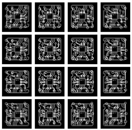
Figure 5. Different views from sources in a $4\times 4$ array of sources.

We chose a small regularization parameter $\lambda =0.1$ to ensure the solution’s stability and uniqueness without significantly biasing the reconstruction. We carefully tuned the step size, $\gamma ={10}^{-9}$, to be sufficiently small, reducing the risk of algorithmic overshooting during optimization. We included additional plots in Appendix A.1 to illustrate the sensitivity of the algorithm to variations in the parameters. Additionally, we manually adjusted the stopping threshold, $ϵ=0.001$, to ensure that the algorithm stops at approximately consistent convergence points. The initial value of the parameter vector $\mathit{\beta }$ is initialized either with a vector or with i.i.d. uniform random values in $[0,1]$. We refer to these methods as EKSD(K) and EKSDR(K), respectively. In several experiments, we will compare the results to completely random designs of K out of N source positions. We refer to this as the RANDOM method.

7.2. Data Set

As a benchmark example, we consider a two-layer PCB of size $80\times 250\times 250$ pixels. It consists of two distinct wire designs (as illustrated in Figure 6) with a thickness of 25 pixels each. These designs are separated by a gap of 20 pixels. The layer of interest is the one depicted in Figure 6a.

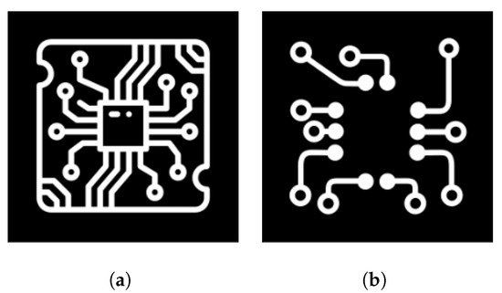
Figure 6. The wire designs with a size of $250\times 250$. (a) Bottom layer of the PCB. (b) Top layer of the PCB.

We create 200 defect shapes in various locations, forming a data set of defective wire design for the bottom layer. A few samples of this data set are depicted in Figure 7. We use half of this data set for source design (calibration) and half for validation.

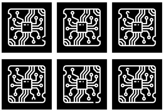
Figure 7. Various defects in different locations on the wire design.

7.3. Convergence

We evaluate the convergence behavior of the EKSD algorithm across various iterations. Here, we let $K=10$, $N=16$, and $D=4L$. In Figure 8, we depict the NMSE at each iteration as evaluated on the calibration (left) and validation (right) data. This figure shows that the design is not overfitted on the calibration data.

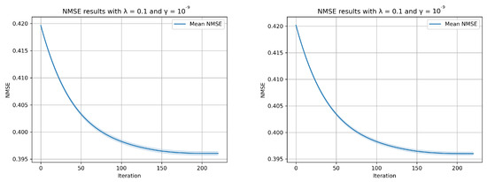
Figure 8. The EKSD algorithm’s convergence as applied to a calibration data set is depicted. The blue line indicates the mean values, while the black dots highlight the variance in the NMSE at each iteration.

7.4. Exploring the Effects of Array Length

Here, we study the influence of the array length D on the reconstruction error for $N=16,36,64$. Hence, we compare the average NMSE over the validation data across various array lengths, as depicted in Figure 9. The heightened errors observed for both smaller and larger array lengths indicate that certain source positions within the array contribute to artifacts in the depth image, leading to an elevated NMSE. Next, we will examine the results for array lengths of $2.4L$ and $4L$, which serve as examples of optimal and suboptimal array lengths, respectively.

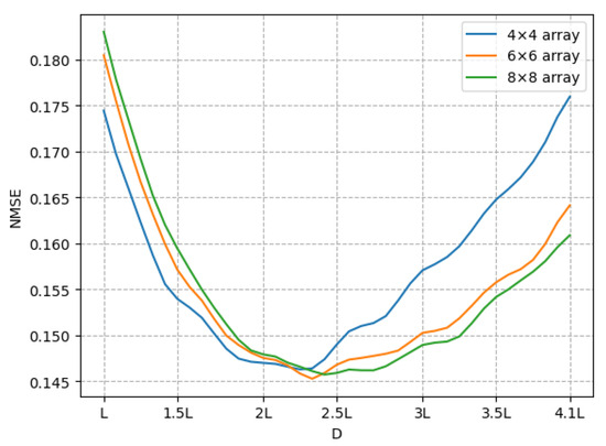
Figure 9. The reconstruction error for various ranges of the area occupied by the source.

7.5. Exhaustive Search

Before evaluating the OED method for a large number of source positions, we aimed to assess its efficiency by comparing it with a combinatorial optimization method. We carried out an exhaustive search to assess the performance of EKSD. We considered $N=16$ source positions with $D=4L$. Figure 10 shows the average NMSE over the validation data for all possible K-source designs for each K, as well as the average NMSE achieved by the EKSD-design. We see the designs found by EKSD are nearly optimal.

Figure 10. The error range applies to any K-source positions within the array of 16 positions, where K can be 4, 6, 8, or 10.

7.6. Source Design 1

We consider three configurations with $N=16,36,64$ at $D=4L$, and we show the NMSE and SSIM results in Table 1. Initially, we display results for depth-reconstructed images utilizing all source positions within the array. Subsequently, we derive $K=10$ efficient source designs with EKSD and EKSDR and present the corresponding NMSE and SSIM results. For each value of N, we observe that EKSD and EKSDR outperform the case using all source positions. This enhancement is largely attributed to the reduction in imaging artifacts, which likely results from the selective measurement approach inherent in EKSD and EKSDR strategies. As a comparison, we show the average NMSE and SSIM of random designs with $K=10$ sources, which significantly underperform compared to the other methods.

Table 1. NMSE and SSIM results with the occupied array length of $4L$. For randomized methods, we present the average and standard deviation over 50 runs.

Source Design	NMSE (N)			SSIM (N)
	$\mathit{N}=\mathbf{16}$	$\mathit{N}=\mathbf{36}$	$\mathit{N}=\mathbf{64}$	$\mathit{N}=\mathbf{16}$	$\mathit{N}=\mathbf{36}$	$\mathit{N}=\mathbf{64}$
ALL ($K=N$)	$0.1749$	$0.1632$	$0.1603$	$0.5630$	$0.5921$	$0.6046$
EKSD ($K=10$)	$0.1611$	$0.1508$	$0.1528$	$0.6275$	$0.7304$	$0.7397$
EKSDR ($K=10$)	$0.1611\pm 3\times {10}^{-4}$	$0.1508\pm 4\times {10}^{-4}$	$0.1518\pm 1.1\times {10}^{-3}$	$0.6275\pm 3\times {10}^{-4}$	$0.7304\pm 4\times {10}^{-4}$	$0.7380\pm 4.6\times {10}^{-3}$
RANDOM ($K=10$)	$0.1819\pm 7\times {10}^{-3}$	$0.1781\pm 1.1\times {10}^{-2}$	$0.1759\pm 1.4\times {10}^{-2}$	$0.57\pm 1.5\times {10}^{-2}$	$0.6075\pm 2.1\times {10}^{-2}$	$0.6248\pm 3\times {10}^{-2}$

Figure 11 shows the corresponding depth images of the bottom layer reconstructed with different source positions. As demonstrated in Section 2.3, artifacts in these images are attributed to the superposition of features from different layers. The lack of rotational acquisition in laminography leads to this artifacts. Clearly, the designs proposed by EKSD minimize artifacts in depth images compared to random designs, facilitating accurate defect detection within the depth images.

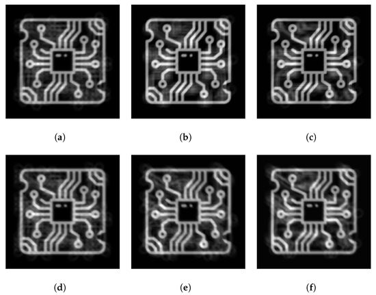
Figure 11. Depth images in (a–c) are reconstructed using 10 proposed source positions from the total of 16, 36, and 64 positions, respectively. Conversely, the depth images in (d–f) are derived from 10 random source positions out of the same total positions.

7.7. Source Design 2

We repeat the previous experiment with the array length optimally chosen according to Figure 9; $D=2.4L$ for different N values. The results are summarized in Table 2. As the full designs are already optimal in a sense, there is less dramatic improvement when optimizing the design with fewer source positions. However, the results for $N=64$ suggest that increasing the number of positions while maintaining a fixed array length, thereby reducing the distance between sources, may result in a non-binary solution. Then, converting the solution into a sparse vector with $K=10$ elements results in a less optimal outcome. The proposed source designs and corresponding depth images are shown in Figure 12.

Table 2. NMSE and SSIM results with the occupied array length of $2.4L$. For randomized methods, we present the average and standard deviation over 50 runs.

Source Design	NMSE (N)			SSIM (N)
	$\mathit{N}=\mathbf{16}$	$\mathit{N}=\mathbf{36}$	$\mathit{N}=\mathbf{64}$	$\mathit{N}=\mathbf{16}$	$\mathit{N}=\mathbf{36}$	$\mathit{N}=\mathbf{64}$
ALL ($K=N$)	$0.1467$	$0.1454$	$0.1459$	$0.7030$	$0.7174$	$0.7233$
EKSD ($K=10$)	$0.1488$	$0.1478$	$0.1548$	$0.7230$	$0.7271$	$0.7011$
EKSDR ($K=10$)	$0.1488\pm 5\times {10}^{-4}$	$0.1484\pm 9\times {10}^{-4}$	$0.1530\pm 2.5\times {10}^{-3}$	$0.7230\pm 5\times {10}^{-4}$	$0.7259\pm 2.7\times {10}^{-3}$	$0.7040\pm 4.7\times {10}^{-3}$
RANDOM ($K=10$)	$0.1537\pm 4\times {10}^{-3}$	$0.1580\pm 5\times {10}^{-3}$	$0.1614\pm 8\times {10}^{-3}$	$0.7040\pm 1\times {10}^{-2}$	$0.7178\pm 1.1\times {10}^{-2}$	$0.7237\pm 1.5\times {10}^{-2}$

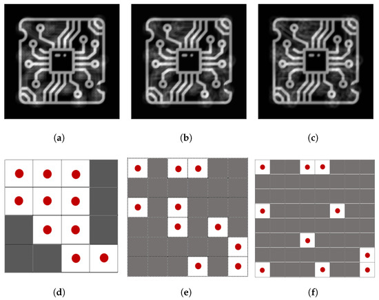
Figure 12. Depth images shown in (a–c) are reconstructed by 10 proposed source positions shown in (d–f), respectively.

8. Discussion

In this research, we explore the methodology of experimental design for a laminographic setup, acknowledging potential challenges that may arise in real-world applications. Here, we outline several significant challenges with our proposed method: (i) As observed in the differences in EKSD and EKSDR results, the non-convex nature of the objective function may lead to entrapment in local minima. To mitigate this issue, one could explore the use of optimization methods that thoroughly explore the entire search space, such as the Genetic Algorithm [18], which can potentially provide more robust solutions by avoiding suboptimal local minima. However, it is worth mentioning that these methods are restricted to low-dimensional problems. (ii) Our method optimizes the positions of sources within a specified grid. However, this grid may not represent the most efficient set of source positions for optimization. An alternative approach could involve optimizing within a continuous domain of positions, leveraging the closed-form formulation for depth image reconstruction presented in this paper. (iii) While our current investigation of the experimental design problem uses noise-free measurements, this assumption may not hold in real-world scenarios characterized by noisy data. This can be addressed by incorporating noise directly into the optimization process to enhance real-world applicability.

9. Conclusions

In real-world scenarios, imaging a particular depth of a planar object can yield valuable information with less effort than a full 3D reconstruction. In a depth image, the information corresponding to the chosen layer appears sharp, while the details of other layers appear blurred. We argue that source design plays a role in mitigating these unwanted artifacts and pose the experimental design problem as a bilevel optimization problem. To solve this problem, we employed bilevel optimization and implemented it using gradient-based methods. The suggested framework can be tailored more specifically to a particular application by incorporating different regularization terms in the lower-level optimization problem or by adopting the alternate loss function in the upper-level optimization problem to more effectively capture the characteristics of the image.

Appendix A.1. Parameter Tuning Plots

In Figure A1, we provide the convergence behavior of our method for distinct values of $\lambda$ and $\gamma$, presenting both the average values (represented by solid points) and the standard deviations (illustrated as shaded areas), with respect to the normalized mean square error (NMSE) in each iteration.

Figure A1. Various $\gamma$ and $\lambda$ applied to the Algorithm 1 and results in different convergence speed.

Figure A1. Various $\gamma$ and $\lambda$ applied to the Algorithm 1 and results in different convergence speed.

Appendix A.2. Forward Operator for the 3D Object

Figure 2 presents the 2D view of the acquisition setup for a planar object $x\left(\mathit{u},z\right)$ where $\mathit{u}\in {\mathbb{R}}^2$ is the lateral coordinate and $z\in \mathbb{R}$ the depth coordinate. The line integral of $x\left(\mathit{u},z\right)$ from $\left(\mathit{s},h\right)$ to $\left(\mathit{r},0\right)$ for a fixed h can be expressed as follows:

$$\begin{array}{c}\hfill y\left(\mathit{r},\mathit{s}\right)=\int x\left(\mathit{s}+\left(\mathit{r}-\mathit{s}\right)t,h-ht\right)\mathrm{d}t\end{array}$$

(A1)

where $\mathit{s}\in {\mathbb{R}}^2$ and $\mathit{r}\in {\mathbb{R}}^2$ denote the source and detector positions, respectively. Next, we substitute $x(\mathit{u},z)$ with its representation in the Fourier domain ${\mathcal{F}}_{3D}\left(x\right)(\mathit{\xi },\zeta )$:

$$\begin{array}{c}\hfill x(\mathit{u},z)=\int \int {\mathcal{F}}_{3D}\left(x\right)\left(\mathit{\xi },\zeta \right)e^{j2\pi \left({\mathit{\xi }}^{\top }\mathit{u}+\zeta z\right)}\mathrm{d}\mathit{\xi }\mathrm{d}\zeta ,\end{array}$$

(A2)

Using (A2) in (A1), it yields

$$\begin{array}{c}\hfill y(\mathit{r},\mathit{s})=\int {\mathcal{F}}_{3D}\left(x\right)\left(\mathit{\xi },\zeta \right)e^{j2\pi \left({\mathit{\xi }}^{\top }\left(\mathit{s}+\left(\mathit{r}-\mathit{s}\right)t\right)+\zeta \left(h-ht\right)\right)}\mathrm{d}t\mathrm{d}\mathit{\xi }\mathrm{d}\zeta ,\end{array}$$

(A3)

Using $\int e^{j2\pi \left({\mathit{\xi }}^{\top }\left(\mathit{r}-\mathit{s}\right)-\zeta h\right)t}\mathrm{d}t=\delta \left({\mathit{\xi }}^{\top }\left(\mathit{r}-\mathit{s}\right)-\zeta h\right)$, it follows that

$$\begin{array}{c}\hfill y(\mathit{r},\mathit{s})=\int {\mathcal{F}}_{3D}\left(x\right)\left(\mathit{\xi },\zeta \right)e^{j2\pi \left({\mathit{\xi }}^{\top }\mathit{s}+\zeta h\right)}\delta \left({\mathit{\xi }}^{\top }\left(\mathit{r}-\mathit{s}\right)-\zeta h\right)\mathrm{d}\zeta \mathrm{d}\mathit{\xi },\end{array}$$

(A4)

and then

$$\begin{array}{c}\hfill y(\mathit{r},\mathit{s})=\int {\mathcal{F}}_{3D}\left(x\right)\left(\mathit{\xi },h^{-1}\mathit{\xi }(\mathit{r}-\mathit{s})\right)e^{j2\pi {\mathit{\xi }}^{\top }\mathit{r}}\mathrm{d}\mathit{\xi }\end{array}$$

(A5)

Using $\mathit{o}=\mathit{r}-\mathit{s}$, the following can be written:

$$\begin{array}{c}\hfill g(\mathit{r},\mathit{o})=\int {\mathcal{F}}_{3D}\left(x\right)\left(\mathit{\xi },h^{-1}{\mathit{\xi }}^{\top }\mathit{o}\right)e^{j2\pi {\mathit{\xi }}^{\top }\mathit{r}}\mathrm{d}\mathit{\xi }\end{array}$$

(A6)

which means we can link the 3D Fourier transform of x to the 2D Fourier transform of the data as

$$\begin{array}{c}\hfill {\mathcal{F}}_{2D}\left(g\right)(\mathit{\xi },\mathit{o})={\mathcal{F}}_{3D}\left(x\right)\left(\mathit{\xi },h^{-1}{\mathit{\xi }}^{\top }\mathit{o}\right).\end{array}$$

(A7)

Appendix A.3. Forward Operator for a 2D Slice at Depth z

We introduce $x_z$ as a slice of the object x at depth z, i.e.,

$$x(\mathit{u},z^{\prime })=x_z\left(\mathit{u}\right)\delta (z^{\prime }-z).$$

We then define the forward operator ${\mathcal{A}}_z$ as projecting a 2D object to the detector at $z=0$ via

$$\begin{array}{c}\hfill y\left(\mathit{r},\mathit{s}\right)=x_z\left(\mathit{s}+\left(1-h^{-1}z\right)\left(\mathit{r}-\mathit{s}\right)\right)\end{array}$$

(A8)

or, equivalently, as

$$\begin{array}{c}\hfill y\left(\mathit{r},\mathit{s}\right)=x_z\left(\mathit{r}\left(1-h^{-1}z\right)+h^{-1}z\mathit{s}\right).\end{array}$$

(A9)

The adjoint operator ${\mathcal{A}}_z^{\ast }$ can be obtained by considering the definition ${⟨{\mathcal{A}}_z{x}_z,y⟩}_{(\mathit{s},\mathit{r})}={⟨x_z,{\mathcal{A}}_z^{\ast }y⟩}_{\mathit{v}}$. First, we have

$$\begin{array}{cc}\hfill & {⟨{\mathcal{A}}_z{x}_z,y⟩}_{(\mathit{s},\mathit{r})}=\hfill \\ \hfill & \int \int x_z\left(\mathit{r}\left(1-h^{-1}z\right)+h^{-1}z\mathit{s}\right)y\left(\mathit{r},\mathit{s}\right)\mathrm{d}\mathit{r}\mathrm{d}\mathit{s}.\hfill \end{array}$$

(A10)

Now, let $\mathit{v}=\mathit{r}\left(1-h^{-1}z\right)+h^{-1}z\mathit{s}$; then, $\mathit{r}=\frac{\mathit{v}-h^{-1}z\mathit{s}}{1-h^{-1}z}$ and $\mathrm{d}\mathit{r}=\frac{1}{1-h^{-1}z}\mathrm{d}\mathit{v}$, and it follows that

$$\begin{array}{cc}& {⟨{\mathcal{A}}_z{x}_z,y⟩}_{(\mathit{s},\mathit{r})}=\hfill \\ \hfill & \frac{1}{1-h^{-1}z}\int \int x_z\left(\mathit{v}\right)y\left(\frac{\mathit{v}-h^{-1}z\mathit{s}}{1-h^{-1}z},\mathit{s}\right)\mathrm{d}\mathit{v}\mathrm{d}\mathit{s}\hfill \\ \hfill & =⟨x_z,{\mathcal{A}}_z^{\ast }y⟩.\hfill \end{array}$$

(A11)

We thus find that ${\mathcal{A}}_z^{\ast }f$ is defined as

$$\begin{array}{c}\hfill \left({\mathcal{A}}_z^{\ast }y\right)\left(\mathit{u}\right)=\frac{1}{1-h^{-1}z}\int y\left(\frac{\mathit{u}-h^{-1}z\mathit{s}}{1-h^{-1}z},\mathit{s}\right)\mathrm{d}\mathit{s}.\end{array}$$

(A12)

By using (A9) in (A12), the composition ${\mathcal{A}}_z^{\ast }{\mathcal{A}}_z$ can be written as below:

$$\begin{array}{c}\hfill \left({\mathcal{A}}_z^{\ast }{\mathcal{A}}_z{x}_z\right)\left(\mathit{u}\right)=\frac{x_z\left(\mathit{u}\right)}{1-h^{-1}z}\int \mathrm{d}\mathit{s}.\end{array}$$

(A13)

Appendix A.4. Back Projection for a Depth Image

We use $y\left(\mathit{r},\mathit{s}\right)$ in (A1) to express ${\mathcal{A}}_z^{\ast }\mathcal{A}$ using (A12):

$$\begin{array}{cc}\hfill & \left({\mathcal{A}}_z^{\ast }\mathcal{A}x\right)\left(\mathit{u}\right)=\hfill \\ \hfill & \frac{1}{1-h^{-1}z}\int \int x\left(\frac{\mathit{u}-h^{-1}z\mathit{s}}{1-h^{-1}z}t+\left(1-t\right)\mathit{s},h\left(1-t\right)\right)\mathrm{d}t\mathrm{d}\mathit{s}.\hfill \end{array}$$

(A14)

Now, let $z^{\prime }=h(1-t)$. Yhen, it can be rewritten as

$$\begin{array}{cc}\hfill & \left({\mathcal{A}}_z^{\ast }\mathcal{A}x\right)\left(\mathit{u}\right)=\hfill \\ \hfill & \frac{1}{h-z}\int \int x\left(\frac{h-z^{\prime }}{h-z}\mathit{u}+\frac{z^{\prime }-z}{h-z}\mathit{s},z^{\prime }\right)\mathrm{d}{z}^{\prime }\mathrm{d}\mathit{s}\hfill \end{array}$$

(A15)

Appendix A.5. Gradient Calculation of the Objective Function

To find the gradient of $\mathit{F}\left(\mathit{\beta }\right):=\frac{1}{2}{\parallel \widehat{\alpha }\left(\mathit{\beta }\right)\widehat{\mathit{x}}\left(\mathit{\beta }\right)-{\mathit{x}}_{\mathrm{gt}}\parallel }^2$ with respect to $\mathit{\beta }$, by the chain roll it reads

$$\begin{array}{c}\hfill \frac{\partial \mathit{F}}{\partial \mathit{\beta }}\left(\mathit{\beta }\right)=\frac{\partial \mathit{F}}{\partial {\widehat{\mathit{x}}}_z}·\frac{\partial {\widehat{\mathit{x}}}_z}{\partial \mathit{\beta }}+\frac{\partial \mathit{F}}{\partial \widehat{\alpha }}·\frac{\partial \widehat{\alpha }}{\partial \mathit{\beta }}\end{array}$$

(A16)

where the second term is equal to zero because $\widehat{\alpha }\left(\mathit{\beta }\right)$ is the optimal point of $\mathit{F}$. Then, the first term can be written as

$$\begin{array}{c}\hfill \frac{\partial \mathit{F}}{\partial \mathit{\beta }}={\left(\frac{\partial {\widehat{\mathit{x}}}_z}{\partial \mathit{\beta }}\right)}^{\top }\frac{\partial \mathit{F}}{\partial {\widehat{\mathit{x}}}_z}=\widehat{\alpha }\left(\mathit{\beta }\right){\left(\frac{\partial {\widehat{\mathit{x}}}_z}{\partial \mathit{\beta }}\right)}^{\top }\left(\widehat{\alpha }\left(\mathit{\beta }\right){\widehat{\mathit{x}}}_z\left(\mathit{\beta }\right)-{\mathit{x}}_{\mathrm{gt}}\right).\end{array}$$

(A17)

To obtain an expression for the derivative of $\widehat{\mathit{x}}$ with respect to $\mathit{\beta }$, we exploit the fact that the lower-level optimization problem (16) has a closed-form solution:

$$\begin{array}{cc}\hfill {\widehat{\mathit{x}}}_z\left(\mathit{\beta }\right)=& {\left({\mathit{A}}_z^{\top }{{\mathit{T}}_{\mathit{\beta }}}^{\top }{\mathit{T}}_{\mathit{\beta }}{\mathit{A}}_z+\lambda \mathit{I}\right)}^{-1}{\mathit{A}}_z^{\top }{{\mathit{T}}_{\mathit{\beta }}}^{\top }{\mathit{T}}_{\mathit{\beta }}\mathit{y}.\hfill \end{array}$$

(A18)

We define ${\mathit{H}}_{\mathit{\beta }}:={\mathit{A}}_z^{\top }{{\mathit{T}}_{\mathit{\beta }}}^{\top }{\mathit{T}}_{\mathit{\beta }}{\mathit{A}}_z+\lambda \mathit{I}$, and then the derivative follows:

$$\begin{array}{c}\hfill \frac{\partial {\widehat{\mathit{x}}}_z\left(\mathit{\beta }\right)}{\partial {\beta }_i}=\frac{\partial {{\mathit{H}}_{\mathit{\beta }}}^{-1}}{\partial {\beta }_i}{\mathit{A}}_z^{\top }{{\mathit{T}}_{\mathit{\beta }}}^{\top }{\mathit{T}}_{\mathit{\beta }}\mathit{y}+{{\mathit{H}}_{\mathit{\beta }}}^{-1}\frac{\partial \left({\mathit{A}}_z^{\top }{{\mathit{T}}_{\mathit{\beta }}}^{\top }{\mathit{T}}_{\mathit{\beta }}\mathit{y}\right)}{\partial {\beta }_i},\end{array}$$

(A19)

Recall that $\frac{\partial {{\mathit{H}}_{\mathit{\beta }}}^{-1}}{\partial {\beta }_i}=-{{\mathit{H}}_{\mathit{\beta }}}^{-1}\frac{\partial {\mathit{H}}_{\mathit{\beta }}}{\partial {\beta }_i}{{\mathit{H}}_{\mathit{\beta }}}^{-1}$; therefore,

$$\begin{array}{c}\hfill \frac{\partial {{\mathit{H}}_{\mathit{\beta }}}^{-1}}{\partial {\beta }_i}=-2{{\mathit{H}}_{\mathit{\beta }}}^{-1}{\mathit{A}}_z^{\top }{{\mathit{T}}_{\mathit{\beta }}}^{\top }\frac{\partial T_{\mathit{\beta }}}{\partial {\beta }_i}{\mathit{A}}_z{{\mathit{H}}_{\mathit{\beta }}}^{-1}\end{array}$$

(A20)

Then, (A19) can be rewritten as

$$\begin{array}{cc}\hfill \frac{\partial {\widehat{\mathit{x}}}_z\left(\mathit{\beta }\right)}{\partial {\beta }_i}& =-2{{\mathit{H}}_{\mathit{\beta }}}^{-1}{\mathit{A}}_z^{\top }{{\mathit{T}}_{\mathit{\beta }}}^{\top }\frac{\partial T_{\mathit{\beta }}}{\partial {\beta }_i}\left({\mathit{A}}_z{{\mathit{H}}_{\mathit{\beta }}}^{-1}{\mathit{A}}_z^{\top }{{\mathit{T}}_{\mathit{\beta }}}^{\top }{\mathit{T}}_{\mathit{\beta }}\mathit{y}-\mathit{y}\right),\hfill \end{array}$$

(A21)

where ${{\mathit{H}}_{\mathit{\beta }}}^{-1}{\mathit{A}}_z^{\top }{{\mathit{T}}_{\mathit{\beta }}}^{\top }{\mathit{T}}_{\mathit{\beta }}\mathit{y}$ is equal to $\widehat{\mathit{x}}\left(\mathit{\beta }\right)$ in (A18) and ${\mathit{H}}_{\mathit{\beta }}^{-1}{\mathit{A}}_z^{\top }{{\mathit{T}}_{\mathit{\beta }}}^{\top }$ is denoted by ${\left({\mathit{T}}_{\mathit{\beta }}{\mathit{A}}_z\right)}_{\lambda }^{†}$. Then, it can be rewritten:

$$\begin{array}{c}\hfill \frac{\partial {\widehat{\mathit{x}}}_z\left(\mathit{\beta }\right)}{\partial {\beta }_i}=2{\left({\mathit{T}}_{\mathit{\beta }}{\mathit{A}}_z\right)}_{\lambda }^{†}\left(\frac{\partial {\mathit{T}}_{\mathit{\beta }}}{\partial {\beta }_i}\left(\mathit{y}-{\mathit{A}}_z\widehat{\mathit{x}}\left(\mathit{\beta }\right)\right)\right)=2{\left({\mathit{T}}_{\mathit{\beta }}{\mathit{A}}_z\right)}_{\lambda }^{†}{\mathit{c}}_i,\end{array}$$

(A22)

For simplicity, we denote $\frac{\partial {\mathit{T}}_{\mathit{\beta }}}{\partial {\beta }_i}\left(\mathit{y}-{\mathit{A}}_z\widehat{\mathit{x}}\left(\mathit{\beta }\right)\right)$ as ${\mathit{c}}_i\in {\mathbb{R}}^m$ and it follows that

$$\begin{array}{c}\hfill \frac{\partial {\widehat{\mathit{x}}}_z\left(\mathit{\beta }\right)}{\partial \mathit{\beta }}=2{\left({\mathit{T}}_{\mathit{\beta }}{\mathit{A}}_z\right)}_{\lambda }^{†}\mathit{C}\end{array}$$

(A23)

where $\mathit{C}=[{\mathit{c}}_1,\dots ,{\mathit{c}}_N]$. The replacement of (A23) into (22) yields

$$\begin{array}{c}\hfill \nabla F=2\widehat{\alpha }\left(\mathit{\beta }\right){\mathit{C}}^{\top }{\left({\mathit{A}}_z^{\top }{\mathit{T}}_{\mathit{\beta }}^{\top }\right)}_{\lambda }^{†}\left(\widehat{\alpha }\left(\mathit{\beta }\right){\widehat{\mathit{x}}}_z\left(\mathit{\beta }\right)-{\mathit{x}}_{\mathrm{gt}}\right).\end{array}$$

(A24)

Appendix A.6. Projection onto the Simplex Constraint

Let $\mathcal{P}$ be an operator that maps each point onto the simplex set of $\mathcal{B}=\{\mathit{u}\in {\mathbb{R}}^m|{\mathit{u}}^{\top }\mathbf{1}=K,0\le u_i\le 1\}$. In fact, the orthogonal projection of $\mathit{p}$ is the unique solution of

$$\begin{array}{c}\hfill \underset{\mathit{t}}{argmin}\frac{1}{2}{\parallel \mathit{t}-\mathit{p}\parallel }^2\mathrm{s}.\mathrm{t}{\mathit{t}}^{\top }\mathbf{1}=K,0\le t_i\le 1,\end{array}$$

(A25)

to solve the above optimization via its dual problem, we introduce the Lagrangian [16]:

$$\begin{array}{c}\hfill \mathcal{L}(\mathit{t},\mu ):=\frac{1}{2}{\parallel \mathit{t}-\mathit{p}\parallel }^2+\mu \left({\mathit{t}}^{\top }\mathbf{1}-K\right),\end{array}$$

(A26)

where $\mu \in \mathbb{R}$ is a Lagrangian multiplier. The dual problem can now be written as

$$\begin{array}{c}\hfill \mathcal{J}\left(\mu \right)=\underset{0\le t_i\le 1}{inf}\mathcal{L}\left(\mathit{t},\mu \right),\end{array}$$

(A27)

where $\mathcal{J}\left(\mu \right)$ is the dual function as the minimum value of the Lagrangian over $\mathit{t}$. Regarding strong duality, the optimal solutions of (A25) and (A27) are equal if there exists a dual variable of $\mu \in \mathbb{R}$ that makes (A27) a tight lower bound for (A25). The solution of the dual problem of (A27) can be written as [19]

$${\mathit{t}}^{★}\left(\mu \right)=min\{max\{\mathit{p}-\mu \mathbf{1},\mathbf{0}\},\mathbf{1}\}$$

where $\mu \in \mathbb{R}$ is obtained by solving ${\mathit{t}}^{★}{\left(\mu \right)}^{\top }\mathbf{1}=K$. Let us define the function $w\left(\mu \right)={\sum }_{i}min\{max\{p_i-\mu ,0\},1\}-K$, which is non-increasing and can be solved using the Newton method. The derivative is given by

$$w^{\prime }\left(\mu \right)=\left|\mathcal{I}\right|,\mathcal{I}=\{i\in \{0,\dots ,n\}:0\le p_i-\mu \le 1\}.$$

References

- Medici, V.; Martarelli, M.; Paone, N.; Pandarese, G.; van de Kamp, W.; Verhoef, B.; Sipsas, K.; Broechler, R.; Besada, L.B.; Alexopoulos, K.; et al. Integration of Non-Destructive Inspection (NDI) systems for Zero-Defect Manufacturing in the Industry 4.0 & IoT (MetroInd4.0&IoT). In Proceedings of the 2023 IEEE International Workshop on Metrology for Industry 4.0 & IoT (MetroInd4.0&IoT), Brescia, Italy, 6–8 June 2023; pp. 439–444. [Google Scholar] [CrossRef]
- Wang, B.; Zhong, S.; Lee, T.L.; Fancey, K.S.; Mi, J. Non-destructive testing and evaluation of composite materials/structures: A state-of-the-art review. Adv. Mech. Eng. 2020, 12, 1687814020913761. [Google Scholar] [CrossRef]
- Hassler, U.; Oeckl, S.; Bauscher, I. Inline ct methods for industrial production. In Proceedings of the International Symposium on NDT in Aerospace 2008, Fürth, Germany, 3–5 December 2008; pp. 123–131. [Google Scholar]
- Gondrom, S.; Zhou, J.; Maisl, M.; Reiter, H.; Kröning, M.; Arnold, W. X-ray computed laminography: An approach of computed tomography for applications with limited access. Nucl. Eng. Des. 1999, 190, 141–147. [Google Scholar] [CrossRef]
- O’Brien, N.; Mavrogordato, M.; Boardman, R.; Sinclair, I.; Hawker, S.; Blumensath, T. Comparing cone beam laminographic system trajectories for composite NDT. Case Stud. Nondestruct. Test. Eval. 2016, 6, 56–61. [Google Scholar] [CrossRef][Green Version]
- Chaloner, K.; Verdinelli, I. Bayesian Experimental Design: A Review. Stat. Sci. 1995, 10, 273–304. [Google Scholar] [CrossRef]
- Haber, E.; Magnant, Z.; Lucero, C.; Tenorio, L. Numerical methods for A-optimal designs with a sparsity constraint for ill-posed inverse problems. Comput. Optim. Appl. 2012, 52, 293–314. [Google Scholar] [CrossRef]
- Haber, E.; Horesh, L.; Tenorio, L. Numerical methods for experimental design of large-scale linear ill-posed inverse problems. Inverse Probl. 2008, 24, 055012. [Google Scholar] [CrossRef]
- Haber, E.; Horesh, L.; Tenorio, L. Numerical methods for the design of large-scale nonlinear discrete ill-posed inverse problems. Inverse Probl. 2009, 26, 025002. [Google Scholar] [CrossRef]
- Ruthotto, L.; Chung, J.; Chung, M. Optimal Experimental Design for Inverse Problems with State Constraints. SIAM J. Sci. Comput. 2018, 40, B1080–B1100. [Google Scholar] [CrossRef]
- van Aarle, W.; Palenstijn, W.J.; Cant, J.; Janssens, E.; Bleichrodt, F.; Dabravolski, A.; Beenhouwer, J.D.; Batenburg, K.J.; Sijbers, J. Fast and flexible X-ray tomography using the ASTRA toolbox. Opt. Express 2016, 24, 25129–25147. [Google Scholar] [CrossRef] [PubMed]
- Jørgensen, J.S.; Lionheart, W.R.B. Chapter 6: Filtered Back-Projection. In Computed Tomography: Algorithms, Insight, and Just Enough Theory; Society for Industrial and Applied Mathematics: Philadelphia, PA, USA, 2021; pp. 73–103. [Google Scholar] [CrossRef]
- Zhang, F. The Schur Complement and Its Applications; Springer Science & Business Media: Berlin/Heidelberg, Germany, 2006; Volume 4. [Google Scholar]
- Paige, C.C.; Saunders, M.A. LSQR: An algorithm for sparse linear equations and sparse least squares. ACM Trans. Math. Softw. (TOMS) 1982, 8, 43–71. [Google Scholar] [CrossRef]
- Sinha, A.; Malo, P.; Deb, K. A Review on Bilevel Optimization: From Classical to Evolutionary Approaches and Applications. IEEE Trans. Evol. Comput. 2018, 22, 276–295. [Google Scholar] [CrossRef]
- Boyd, S.; Vandenberghe, L. Convex Optimization; Cambridge University Press: Cambridge, UK, 2004. [Google Scholar]
- Wang, Z.; Bovik, A.; Sheikh, H.; Simoncelli, E. Image quality assessment: From error visibility to structural similarity. IEEE Trans. Image Process. 2004, 13, 600–612. [Google Scholar] [CrossRef] [PubMed]
- Srinivas, M.; Patnaik, L. Genetic algorithms: A survey. Computer 1994, 27, 17–26. [Google Scholar] [CrossRef]
- Kadu, A.; van Leeuwen, T.; Batenburg, K.J. CoShaRP: A convex program for single-shot tomographic shape sensing. Inverse Probl. 2021, 37, 105005. [Google Scholar] [CrossRef]
Disclaimer/Publisher’s Note: The statements, opinions and data contained in all publications are solely those of the individual author(s) and contributor(s) and not of MDPI and/or the editor(s). MDPI and/or the editor(s) disclaim responsibility for any injury to people or property resulting from any ideas, methods, instructions or products referred to in the content. |
© 2024 by the authors. Licensee MDPI, Basel, Switzerland. This article is an open access article distributed under the terms and conditions of the Creative Commons Attribution (CC BY) license (https://creativecommons.org/licenses/by/4.0/).