Article

A Sustainable Supply Chain Model with a Setup Cost Reduction Policy for Imperfect Items under Learning in a Cloudy Fuzzy Environment

by
Basim S. O. Alsaedi
Department of Statistics, University of Tabuk, Tabuk 71491, Saudi Arabia
Mathematics 2024, 12(10), 1603; https://doi.org/10.3390/math12101603
Submission received: 30 March 2024 / Revised: 1 May 2024 / Accepted: 7 May 2024 / Published: 20 May 2024

Abstract

:
The present paper deals with an integrated sustainable supply chain model with the effect of learning for an imperfect production system under a cloudy fuzzy environment where the demand rate is treated as a cloudy triangular fuzzy (imprecise) number, which means that the demand rate of the items is not constant, and shortages and a warranty policy are allowed. The vendor governs the manufacturing process to serve the demand of the buyer. When the vendor supplies the demanded lot after the production of items, it is also considered that the delivery lots have some defective items that follow an S-shape learning curve. After receiving the lot, the buyer inspects the whole lot, and the buyer classifies the whole lot into two categories: one is the defective-quality items and the other is the imperfect-quality items. The buyer returns the defective-quality items to the seller after a screening process, for which a warranty cost is included. During the transportation of the items, a lot of carbon units are emitted from the transportation, damaging the quality of the environment. The seller includes carbon emission costs to achieve sustainability as per considerations. A one-time discrete investment is also included for the minimizing of the setup cost of the seller for the next cycles. We developed models for the scenario of the separate decision and for the integrated decision of the players (seller/buyer) under the model’s consideration. Our aim is to jointly optimize the integrated total fuzzy cost under a cloudy fuzzy environment sustained by the seller and buyer. Numerical examples, sensitivity, analysis limitations, future scope and conclusions have been provided for the justification of the proposed model, and the impact of the input parameters on the decision variables and integrated total fuzzy cost for the supply chain are provided for the validity and robustness of this proposed model. The effect of learning in a cloudy fuzzy environment was positive for this proposed model.

1. Short Outlook of the Abstract through a Flowchart

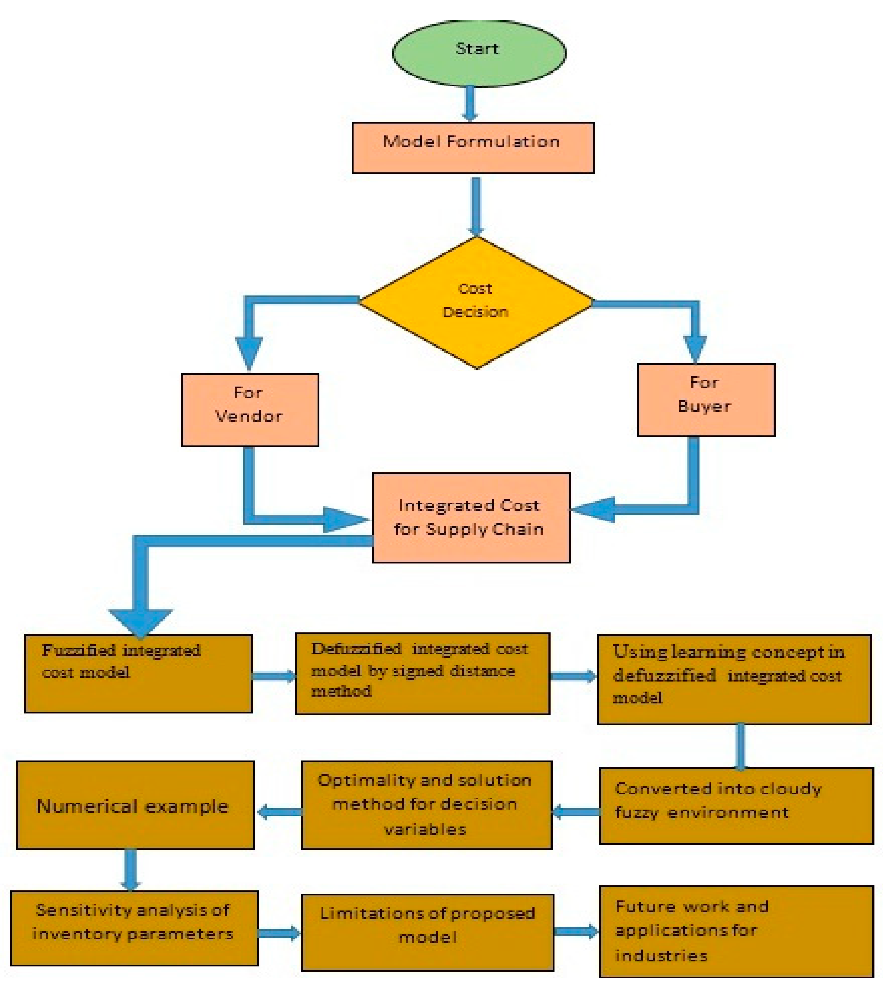
This section explains the buyer’s plan and seller’s plan individually and in an integrated form through a flowchart and presented in the Figure 1.

2. Explanation of the Proposed Model through a Flowchart

This section presents the entire strategy of the proposed model from top to bottom through a flowchart. The strategy of the buyer and seller, which is given below in Figure 2, is also explained.

3. Basic Introduction

Generally, production companies want to supply 100% good-quality items after production as per demanded orders, but in actuality, companies cannot supply 100% good-quality items to the clients due to problems like machines stopping unfortunately in the absence of electricity or due to some faults in production system or the storage of the raw material without any preservation system for the production and the quality of the storage items being damaged as time passes. For this reason, during the production of items, some defective items that have low value as good-quality items are obtained, and some companies incorporate waste management costs for the maintaining of profit. When defective items are not suitable for rework, then they are delivered to the disposal section, and the companies manage the loss from the disposal items by including disposal costs. A green environment is more beneficial for human life, and nowadays, a lot of carbon units in the form of gases damage the green quality of the environment. Carbon units are emitted from different sources like meat factories, food factories, transportation of items through different vehicles, burning of vehicle oils, etc. Carbon emissions negatively affect the supply chain, and this impact can be reduced by using a decision strategy and also incorporating carbon emission costs. Setup management for any business is an effective decision because it affects the system’s inventory cost. The setup cost is reduced for the next cycle by using a one-time discrete investment policy and accounting for the imprecise nature of the demand rate with the help of the cloudy fuzzy technique. The learning effect is one type of mathematical tool that observes repetitions of a task, and learning in a fuzzy technique is incorporated in this study. In this study, we incorporated some realistic situations like imperfect production, carbon emissions, a one-time discrete investment policy and the impact of learning and a cloudy fuzzy environment. We calculated order quantity, backorders and number of freights for the supply chain under a cloudy fuzzy environment and treated them as decision variables. We optimized the integrated total fuzzy cost with respect to order quantity, backorders, number of freights and investment setup cost where order quantity, backorders, number of freights and investment setup cost are treated as decision variables.
The rest of this manuscript is structured as follows: (i) Section 3.1, Section 3.2, Section 3.3, Section 3.4, Section 3.5 and Section 3.6 present a lot of literature reviews, which are the basis of the proposed model, and Section 3.7 presents the research gap and also proposed work of this paper; (ii) Section 2 provides the notations and assumptions for this proposed model; (iii) Section 3 provides the model optimization and solution method; (iv) Section 4 reflects the numerical example for the justification of the proposed model; (v) Section 5 represents the sensitivity of the input parameters and also explains the observation and managerial insights; (vi) Section 6 reveals the summary of the results of the proposed model and also provides the future work of this model; (vii) Section 7 shows the limitations of the proposed work; (viii) Section 7.1 gives the applications and practical implications of this proposed work; (ix) Section 7.6 provides the social implications of this research study.
For the development of the proposed model, we studied a lot of literature reviews which motivated us to fill the research gap and design new research for a new generation. In this direction, many more authors worked and developed inventory models for new generations. We discuss some literature reviews in the forthcoming subsection which are the backbone of this model.

3.1. EOQ and Imperfection Literature Review

We discuss only studies that are related to imperfect-quality items, and in this field, a lot of authors have worked with nice contributions. In this subsection, we select some renowned authors. Salameh and Jaber [1] proposed an ordering policies model by using of inspection process. Biel, K., Glock [2] to solve for the predicted full worth per unit of time, during supply chain model and Jaggi and Mittal [3] also gave good contribution for the imperfect quality items. The numerous current studies have properly assumed—with unrealistic implications for supply chain management—that shortages are not acceptable. Unexpected requests or uneven manufacturing capacity may, in fact, occasionally cause shortages, which will affect supplier and store decisions. The model of Salameh and Jaber [1] was expanded upon by Wee et al. [4], who added shortcomings to each cycle. Eroglu and Ozdemir [5] expanded on Salameh and Jaber’s [1] research to take into account goods of lower quality during shortages. Roy et al. [6] and Sarkar [7] created an inventory model for deteriorating products of poor quality that were subjected to an inspection procedure, using faulty items as random variables. Jaggi et al. [8] have refined an EOQ mathematical model for degrading items with faulty quality under inspection when the screening rate is higher than the demand rate. Sebatjane and Adetunji [9] presented an EOQ-based inventory model with imperfect-quality items for growing items where the order quantity was calculated for the ordering policies. Ozturk [10] developed a production-based inventory model with shortage policies for defective items under a rework process and calculated the production quantity. Gautam et al. [11] described an inventory model with defective-quality items for a two-decade review. Jayaswal and Mittal [12] motivated by the literature review of Goutam et al. [11], developed an ordering-policy-based inventory model with inflationary conditions under an inspection process. In this direction, Narang and De [13] designed a production-based inventory model with a rework policy for defective deteriorating items under a genetic algorithm where the demand rate depends on the advertisement, time and selling price. Taleizadeh et al. [14] developed an economic production quantity inventory model for defective items under a rework process where lot size and backorder level were calculated for the system.

3.2. Carbon Emission Literature Review

We have included a review of relevant studies that are based on carbon emissions in this area. An inventory model was provided under the carbon footprint by Tang et al. [15]. Wang et al. [16] provided their research findings based on the CO2 emissions from the world’s space freight in this order. Zhu et al. [17] talked about carbon-footprint-conscious cleaner research for the environment. An inventory model including the impact of fuel cost under carbon emissions was presented by Gurtu et al. [18]. In the three-echelon supply chain model, Sarkar et al. [19] investigated the effects of varying transportation and carbon emissions. A sustainable inventory model for degrading faulty objects under carbon emissions was given by Tiwari et al. [20]. The optimal strategy was outlined by Gautam and Khanna [21] by taking into account that the shipment delivery truck would only be utilized to return the damaged items. For 3D printing, Thomas and Mishra [22] examine a sustainable supply chain model that reduces waste under carbon emissions and minimizes carbon in various plastic manufacturing sectors. Sharma et al. [23] proposed a green supply chain model for defective items under a supply chain model where a rework process is included. In this way, Nobil et al. [24] considered a sustainable inventory model with a shortage policy under a warm-up process.

3.3. Supply Chain Literature Review

We cover a few chosen studies that use various approaches and are based on the supply chain model in this part. An SCM system with inflation and a credit term was presented by Ruidas et al. [25] for perishable goods. The three-level supply chain model under numerous participants was explained by Jaber and Goyal [26]. Khan et al. [27] expanded a few supply chain models into a three-level model by using learning. According to Bazan et al. [28], an SCM system with greenhouse carbon emissions under diverse energy consumption and strategy was anticipated. Two-level supply chain management (SCM) with credit financing was suggested by Sahoo et al. [29] for effective vendor and buyer collaboration.
In a recent case study, Rajput et al. [30] developed an integrated supply chain management (SCM) system for both buyers and sellers by of using of fuzzy theory. This system was sustainable since it took into account the manufacturing of subpar goods and carbon emissions. Subsequently, distinct strategies were offered by Gautam et al. [31], Jamal et al. [32] and Rout et al. [33]. In this field, very recent work was performed by Singh and Goel [34] and this research study developed a supply chain model with a waste management policy under a reverse logistics policy where an inflationary policy is allowed.

3.4. Learning Literature Review

The impact of learning and screening mistakes in the economic production model under supply chain and stochastic lead time as well as fuzzy theory needs was documented by Maity et al. [35]. An inventory model with learning was created by Jaber and Bonney [36] to enhance process quality. An economic production model including the influence of learning in the areas of production, dependability, quality, and energy efficiency was provided by Marchi et al. [37]. The influence of remembering and learning on the viability of implementing additive manufacturing within a supply chain model was examined by Chu et al. [38]. The influence of learning on the order quantity problem under production and group size was demonstrated by Pal et al. [39]. Giri and Masanta [40] suggested a closed-loop supply chain management (SCM) system where the demand rate is a function of price and learning occurs during the inspection process. An EOQ model with inflation and carbon emissions under the influence of learning for deteriorating products was presented by Alamri et al. [41]. Sangal et al. [42] proposed a supply chain model with preservation technology and waste management policy for best-quality items under learning in a fuzzy environment.

3.5. Fuzzy and Cloudy Fuzzy Literature Review

An inventory model including a trade credit term, shortages under fuzzy concepts, and inspection for deteriorating products was described by Jaggi et al. [43]. Jaggi et al. [43] suggested a mathematical model with a fuzzy environment for degrading commodities under shortages where the demand rate depends on time in order to better the study. An EOQ model with a fuzzy environment and trade credit during shortages was enhanced by Jaggi and Sharma [44]. An EOQ model with a fuzzy environment was generalized by Sharma et al. [45] under the refill system policy. An EOQ model with the impact of learning for defective-quality items under fuzzy systems was explained by Patro et al. [46]. An eco-friendly EOQ model with shortages in a fuzzy environment was presented by Bhavani et al. [47]. An EOQ model examining the impact of learning and credit financing policies in a murky, fuzzy environment was given by Jayaswal et al. [48]. Alamri [49] improved a supply chain model with the effect of learning in a fuzzy environment for growing items under a trade credit policy where the demand rate was treated as a triangular fuzzy number. Alsaedi et al. [50] presented a sustainable supply chain model with the effect of carbon emissions for defective items under learning in a fuzzy environment where a setup cost reduction policy is not allowed and calculated the total profit for the supply chain under a recycling process. Padiyar et al. [51] presented a cloudy fuzzy-based supply chain model for a production process under some realistic situations. Mahata et al. [52] considered a three-echelon supply chain model with the effect of learning for defective items under an imperfect production process where inspection error and return policy are allowed. Sugapriya et al. [53] developed a production-based inventory model with an inspection process under a remanufacturing system where backorder and lost sale policies are allowed. Garg et al. [54] generalized an inventory model with a returnable policy under a triangular fuzzy number.

3.6. Our Proposed Work with Research Gap

This section shows the research gap between authors’ contributions and an attempt to fill this research gap by applying recent policies. In this point of view, we studied a lot of studies already mentioned in the literature review subsection, and then we obtained some research articles in which some inventory decisions like imperfect production policy, shortages, investment in setup cost, warranty policy, waste management cost, theory of learning, carbon emissions, setup cost reduction policy and cloudy fuzzy environment and also more realistic situations were not covered. We concentrated on the imperfect-production-based literature and collected some literature from 2018 to 2024 in which some policies have not used our proposed work.
Our proposed work tried to fill the research gap among the authors’ contributions through the mathematical model, and we developed a sustainable supply chain model with a setup cost reduction policy for imperfect items under learning in a cloudy fuzzy environment where a warranty policy is allowed and calculated the total expected fuzzy cost per unit time. Our contributions in this study are presented at the bottom of Table 1.
As per consideration, we need some basic definitions that are useful for the improvement of the proposed study in a cloudy fuzzy environment, and we also need to discuss Wright’s curve, which is related to the learning effect. The following subsection covers all definitions.

3.7. Basic Definitions

All definitions related to the fuzzy environment have been taken from De and Mahata [56], Kazemi et al. [63] and Bjork [64], as we were motivated by their good contribution.
Definition 1.
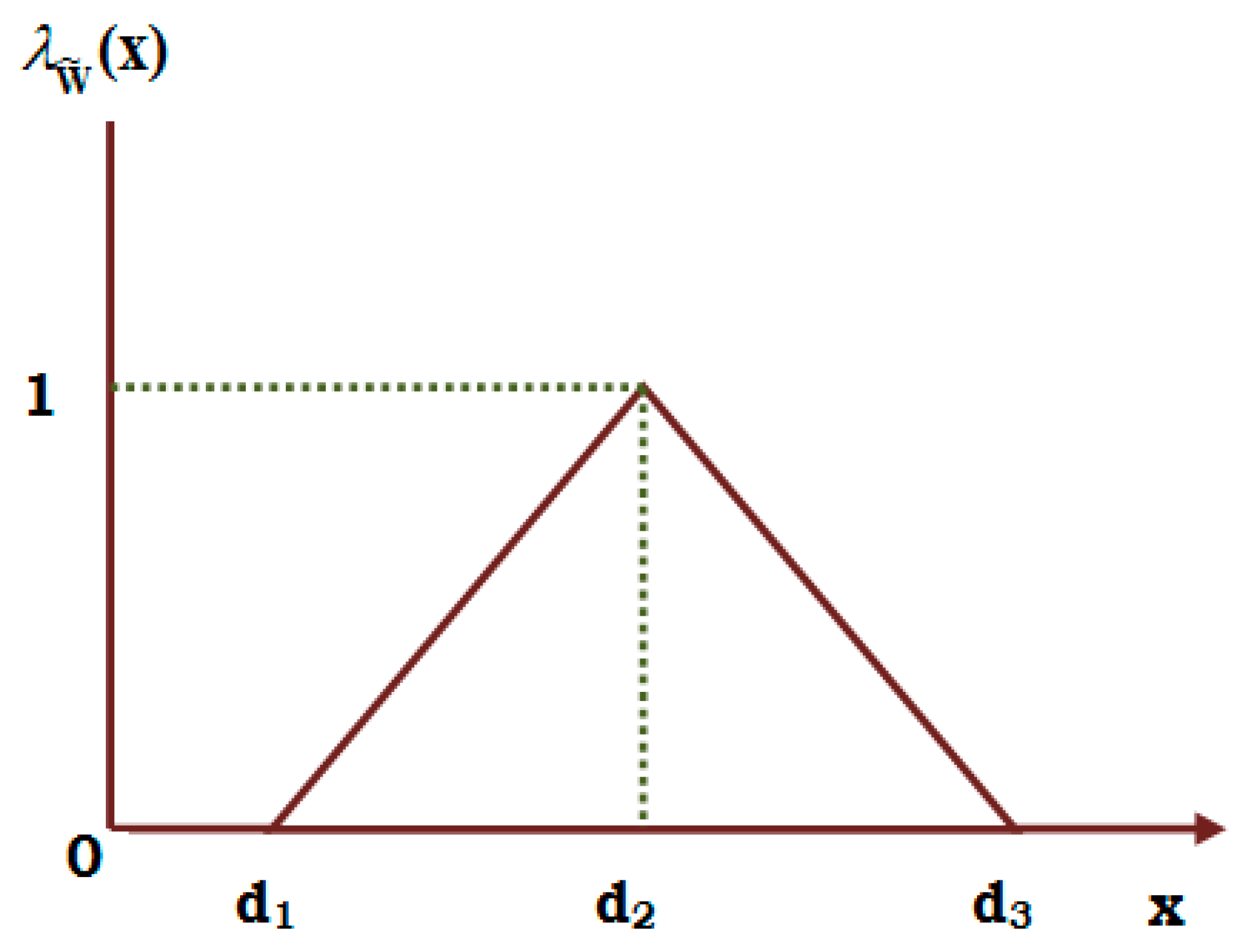
If  R is a universal set and  W  is any set on  R , then a fuzzy set of  W   on  R   is represented by     W ~ ; mathematically, it can be written that    W ~ = x ,   λ   W ~ x : x R , where  λ   W ~   represents a membership function such that  λ   W ~ : R 0 ,   1 . The triplet  d 1 , d 2 , d 3   is used as a triangular fuzzy number, and this number should be related to the condition   d 1 < d 2 < d 3 and it is represented in the Figure 3. The continuous membership function is defined as follows:
λ   W ~ = d d 1 d 2 d 1   d 1 d d 2 d 3 d d 3 d 2   d 2 d d 3 0   O t h e r w i s e
Definition 2.
If   c   is any number and   0   R , then the signed distance from  c   to   0   is   d c , 0 = c , and if   c < 0 ,   then the signed distance from   c   to   0   is   d c , 0 = c .   Let it be assumed that Ω is the family of fuzzy sets   C ~   defined on   R ; then,   α c u t , C α = C L α , C U α   for   α ϵ 0,1 , and  C L α and   C U α   are continuous functions on  α . Then, we can write the value of  C α   as follows:
C α = 0 α 1 C L α α , C U α α
Definition 3.
If   C ~   is the member of Ω, then the signed distance of   C ~   to   0 ~ 1   is given as follows:
d c , 0 = 1 2 0 1 C L α + C U α d α
Definition 4.
If     C ~ = c 1 , c 2 , c 3   is a triangular fuzzy number, then the   α c u t   of     C ~   is   C α = C L α , C U α , where   C L α = c 1 + c 2 c 1 α   and   C U α = c 3 c 3 c 2 α   for     α ϵ 0 ,   1 . The signed distance of     C ~   to   0 ~ 1   is
d   C ~ , 0 = c 1 + 2 c 2 + c 3 2
Definition 5.
For   C ˜ Ω , the signed distance from   B ˜   to   0 ˜ 1   is defined as
d B ˜ , 0 ˜ = 1 2 0 1 B ˜ L α + B ˜ R α   d α
Definition 6.
If   A ˜ = x 1 , x 2 , x 3   is a triangular fuzzy number, then the   α cut of   A ˜   is   A α = A L α , A U α   for   α 0 ,   1   where   A L α = x 1 + x 2 x 1 α   and   A U α = x 3 x 3 x 2 α . Then, the signed distance from   A ˜   to   0 ˜ 1   is
d A ˜ ,   0 ˜ = x 1 + 2 x 2 + x 3 4
Definition 7.
Cloudy fuzzy environment and Yager’s ranking index.
Let us consider that   A ~   is a fuzzy set whose components are the elements of  R × R × R   and also that it belongs to the set of real numbers with the membership grade which satisfies the functional relation μ : R × R [ 0 ,   1 ] . In particular, it is assumed that the set   R   is defined in the time set domain such that   μ : R × T [ 0 ,   1 ] ; now, as   t , if   μ y , t 1   for some   y R   and   t T , then the set   A ~   is called a cloudy fuzzy number. If the fuzzy number   A ~   of the form   A ~ = a 1 , a 2 , a 3   is called a cloudy triangular fuzzy number and if for all   t T ,   μ y , t   reaches the maximum membership degree 1. Then it represents a cloudy normalized triangular fuzzy number or CNTEF and is represented graphically in   Figure 4. Let   B L α   and   B U α   be the left and right   α cuts of a fuzzy number   a ˜ . The defuzzification rule under Yager’s ranking index as suggested by De and Mahata (2019) [56]  is given as follows:
I a ~ = 1 2 0 1 B L α + B R α d α
Definition 8.
Learning curve.
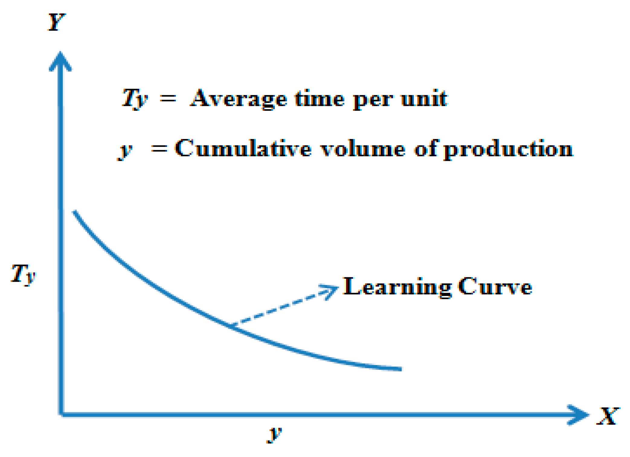
The learning statistical curve has been taken from Wright [65], and the suggested mathematical form of learning is given as follows:
T y = T 1 y b
where T y is the time for the making of the y-th unit, T 1 is the initial time for making y units and b is the slope of the learning parameter. Wright’s learning curve is given in Figure 5.

4. Model’s Assumptions and Notations

In this section, we present the notations and assumptions of the proposed model.

4.1. Notations for the Model Parameters

DDemand rate of the items (unit per year);
D ~ Demand rate in fuzzy environment (unit per year);
Δ H D Upper deviation of demand rate in fuzzy environment (unit per year);
Δ L D Lower deviation of demand rate in fuzzy environment (unit per year);
( D     Δ L D ,   D ,   D   +   Δ H D ) Triangular fuzzy number for the demand rate;
M (Decesion Variable) Order quantity in fuzzy environment (units);
B (Decesion Variable) Backorder lot size in fuzzy environment (units);
WProduction rate of items (unit per year);
NNumber of freights;
αDefective percentage in the ordered lot with uniform probability density function f(α)
AbOrdering cost from buyer side (USD per order);
hbHolding cost from buyer side (USD per unit per year);
SbInspection cost from buyer side (USD per year);
CbBackordering cost from buyer side (USD per year);
hvHolding cost from vendor side (USD per unit per year);
FcFixed carbon emission cost from vendor side (USD per transport);
VcVariable carbon emission cost from vendor side (USD per unit);
FTFixed transportation cost from vendor side (USD per transport);
VTVariable transportation cost from vendor side (USD per unit);
AVInitial setup cost from vendor side (USD per setup);
µInvestment in the setup cost from vendor side;
AV1 (µ) = A V e π µ where π is known input parameterSetup cost from vendor side (USD per setup) after investment;
Ip = A particular investment;
ωv = Unit warranty cost from vendor side for imperfect-quality items;
ωm = Waste management cost for waste-quality items;
l = Learning rate;
n = Number of shipments
Ψb (N, M, B) Total inventory cost for the buyer (USD) side;
ΨbF (N, M, B) Total fuzzy inventory cost for the buyer (USD) side;
ΨbdF (N, M, B) Total defuzzified inventory fuzzy cost for the buyer (USD) side;
ΨV (N, M, µ) Total inventory cost for the vendor (USD) side;
ΨVF (N, M, µ) Total fuzzy inventory cost for the vendor (USD) side;
ΨVdF (N, M, µ) Total defuzzified inventory fuzzy cost for the vendor (USD) side;
ΨI (N, M, B, µ) Total integrated inventory cost for the supply chain (USD);
ΨIF (N, M, B, µ) Total integrated fuzzy inventory cost for the supply chain (USD);
ΨIdF (N, M, B, µ) Total defuzzified integrated fuzzy inventory cost for the supply chain (USD);
ΨIdFL(N, M, B, µ) Total defuzzified integrated fuzzy inventory cost for the supply chain (USD) under learning effect and cloudy fuzzy environment.

4.2. Assumptions for the Model Parameters

In this proposed model, a single vendor, a single buyer and one type of item are assumed in the supply chain.
During transportation, lead time is known and constant for the supply chain.
Shortages are completely backlogged.
In the proposed supply chain model, it is considered that the demand rate of the item is imprecise in nature and also treated as a triangular fuzzy number.
The learning effect is involved in the lower and upper deviation of the fuzzy demand rate under a cloudy fuzzy environment.
Waste management costs are included for waste products from the buyer side.
Fixed and variable costs of carbon emission are included from the vendor side.
The vendor includes the warranty cost ( ω v ) for each imperfect-quality item.
The vendor sells the imperfect-quality item in another market at a low price.
The inspection process is considered as lead time for the supply chain.
The buyer inspects the whole received lot from the vendor for each cycle length and also includes the inspection cost for this task.
The cost of keeping for the buyer decreases as shipping increases, h b n = h 0 + h 1 n χ   , because the holding cost is inversely related to the shipment, where h 0 is the fixed part of the holding cost, h 1 n χ  is the variable holding cost (this part decreases when shipment ( n ) increases) and χ is a constant parameter.
The cost of ordering for the buyer decreases as shipment increases, K = A o + A 2 n χ   , because the ordering cost is inversely related to the shipment, where A is the fixed part of the ordering cost, A 2 n χ   is the variable ordering cost (this part decreases when shipment ( n ) increases) and χ is a constant parameter where  A 0 and A 1 are the fixed ordering cost,   n is the shipment and χ is a supporting parameter.
A particular investment I p is included for reducing the setup cost, and it can be defined, A V 1 µ = A V e π µ w h e r e   π  is a known input parameter and µ is investment in the setup cost from the vendor side. This consideration shows that an increase in investment amount for the supporting of the supply chain lowers the setup cost because the relation between setup cost and investment is inverse.
The lot size of the item M includes defectives. The rate of defectives α follows the probability density function (pdf) f α , and it is also presumed that E α < 1 D W , so as to ensure the manufacturing capacity is enough to fulfill the annual demand of the buyer.
The production process is managed by the vendor, and the produced goods are sent to the buyer in numerous replacements without undergoing an initial screening test. This results in the delivery of a certain quantity of faulty items, which are distributed uniformly.
The carbon emissions resulting from numerous shipments and transportation are considered. We have included a tax for carbon emissions.
The buyer includes the waste management cost due to waste products and reduces the loss from this cost.

5. Mathematical Formulation of Proposed Model

In this section, we discuss the problem definition, which is based on the theoretical description of the fuzzy demand and cost interpretation, the percentage of defectives in the delivered lot, the strategy of the setup cost reduction when a discrete investment is allowed for the minimizing of the setup cost, and extra waste management cost.

5.1. Theoretical Strategy of the Proposed Model

This section presents a theoretical interpretation and the significance of the issue based on the individual and collective perspectives of the seller and the buyer. The issue arises between a vendor, buyer and customer for a certain type of product in a supply chain model. The products in question suggest adhering to a hazy demand curve. Production of the goods is the vendor’s responsibility; the vendor handles the selling process; the customer buys the goods, utilizes them and returns them to the buyer. The abstract flowchart displays the customer’s and seller’s operations. The procedure begins when the buyer makes a purchase. At this point, the holding and ordering costs for the buyer are determined by the cost of shipping, and the nature of the demand rate is imprecise, with lower and upper deviations of demand following the impact of learning. The seller produces the amount that the customer requests and then makes several deliveries to the buyer. There are transportation-related and construction-related carbon emissions. In essence, the given lot contains faulty products that the buyer finds and separates after a first examination. The buyer conducts a firsthand assessment to identify and isolate any defective-quality goods included in the provided batch. Supply chain researchers have launched a clean and sustainable strategy to improve product recovery efforts by using waste management costs. In this paper, we assume that the investment increases and then the setup cost decreases as per policy. Sometimes a lot of products are obtained from the inspection process that are not able to be recycled and are fully damaged. The buyers have to face more losses with these waste products. From these problems, the buyer includes waste management costs. This campaign focuses on encouraging customers to return any worn goods to the seller in order to receive a credit against future purchases. When consecutive lots are received, the buyer is responsible for holding onto the worn and subpar products up until the final conclusion of the shipment cycle, at which point they return them all to the vendor because the vendor includes the warranty cost for each defective item. Finally, the buyer and vendor both benefit from the minimizing of the integrated total fuzzy cost by using the setup cost reduction policy, waste management cost, learning in a cloudy fuzzy environment, carbon emission cost and extra transportation cost.

5.2. Problem Definition of Proposed Model

Considering the current demand trend while maintaining the quality and quantity standards for a certain sort of commodity, the suggested model depends on a single buyer, a single seller and a single customer and takes into account a single item. It is first believed that a fuzzy rate of demand units will be examined by the buyer. The desired supply is M units, which must be handled by the seller and sent in n shipments, each consisting of M units. Because of the unavoidable flaws in the manufacturing lot, the requested shipments may contain some defective goods, resulting in increased warranty costs on the side of the seller. The final customer inspects the lot as soon as the order ships, sorting the flawless pieces from the faulty ones. Let us assume that α is the batch’s defective proportion. The total number of faulty-quality items at the conclusion of the cycle will be α M . Furthermore, purchasing encourages all clients to return the items they have used. It is considered that the buyer requires demand of D   u n i t s in a year for delivery of the items to the customers. The buyer orders fixed batches with a lot size of M p r o d   u n i t s from the vendor for the manufacturing of items, and the vendor takes responsibility for the order demand from the buyer side as per agreement. The vendor plans to ship the demanded quantities to the buyer in N shipments with equal lot size M . Actually, the production system is reconsidered as imperfect, and as per the deal between the vendor and buyer, the delivered lot from the vendor has some defective items in each shipment. The buyer inspects the received entire lot by using a screening process from the vendor side and returns the defectives to the vendor as per agreement. The vendor includes the warranty cost for each defective; in this view, the end demand of the client is satisfied with good-quality items and unsatisfied with imperfect-quality items. The buyer incurs the waste management cost for each defective item that is unable to be recycled, and the price of these items is much less than that of defectives. Shortages are allowed on the buyer side and also considered completely backlogged. The vendor uses transportation for the shipment of the demanded orders from the buyer side and includes fixed and variable transportation as well as carbon emission costs. The prime objective is that both players (vendor and buyer) minimize the integrated fuzzy total cost with respect to the number of shipments ( N ), order quantity M , shortage quantity ( B ) and investment in setup cost ( µ ) under a locked fuzzy environment for the supply chain. For the sustainability of the proposed model, we show the integrated total fuzzy cost, buyer’s total fuzzy cost and vendor’s total fuzzy cost separately and also compare them. In the forthcoming subsection, we discuss the vendor’s strategy outlook, buyer’s strategy outlook and integrated vendor’s strategy outlook.

5.3. Vendor’s Decision Strategy Outlook

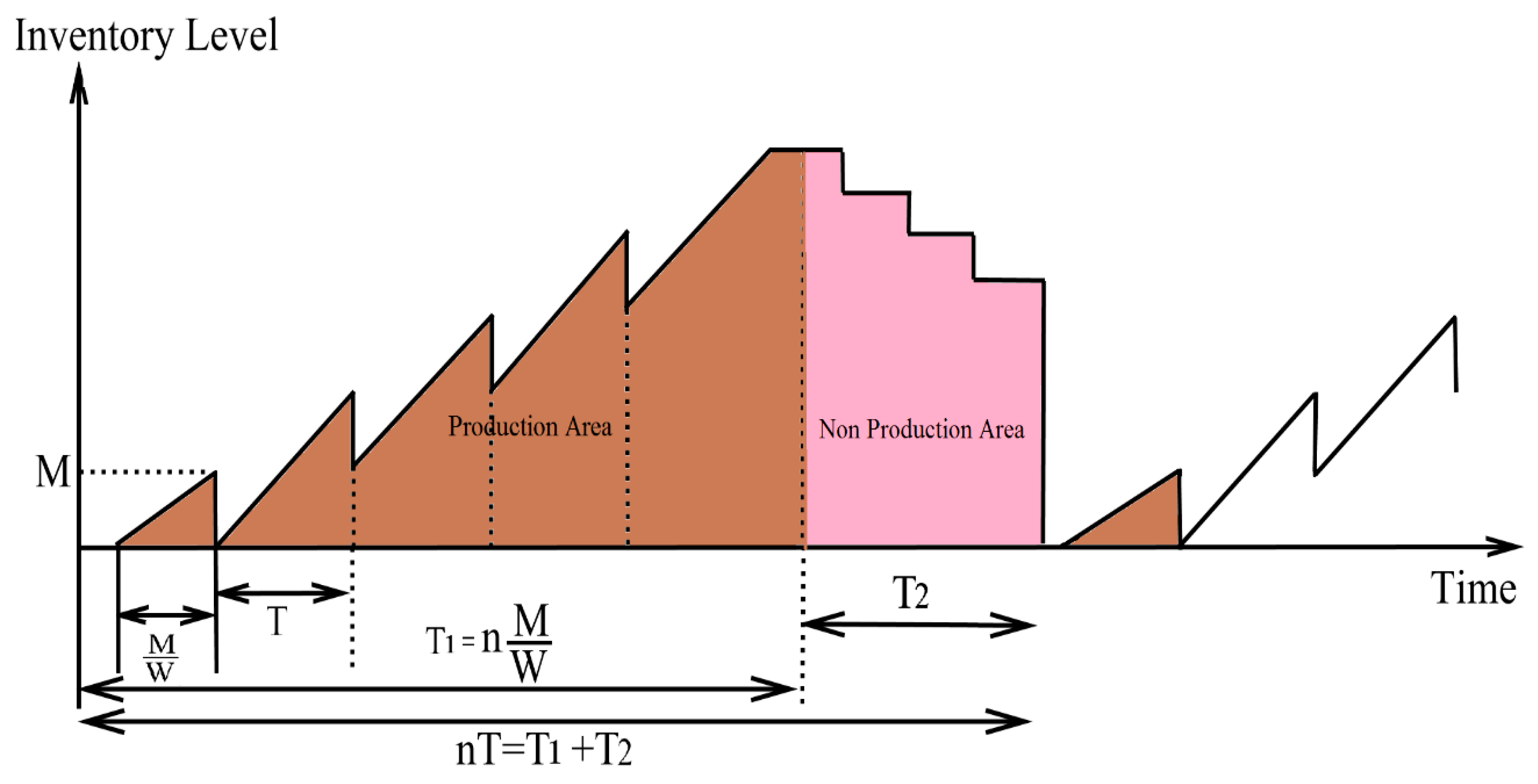
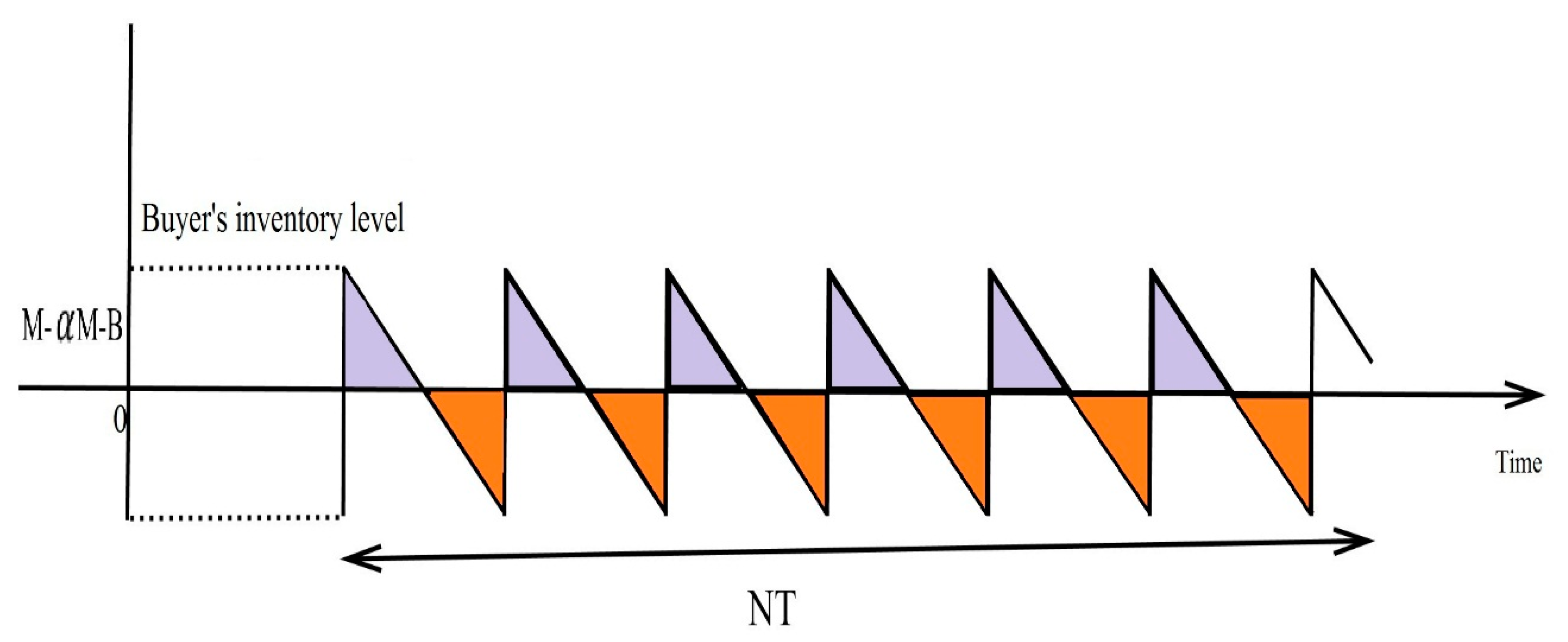
In this section, we discuss the strategy of the vendor for the buyer in the supply chain, and Figure 6 and Figure 7 show the working task of the scenario of the vendor’s strategy over time.
The vendor’s total cost is the sum of the inventory costs of setup S C , holding cost I H C V , fixed transportation cost F T C V , variable transportation cost V T C V , fixed carbon emissions cost F C C V , variable carbon emission cost V C C V , investment in setup μ and warranty cost W C V ; it can be written mathematically as
Ψ V N , M , μ =   Setup S C +   Holding   cost I H C V + Fixed   transportation   cost F T C V + V a r i a b l e   t r a n s p o r t a t i o n   c o s t V T C V   + F i x e d   c a r b o n   e m i s s i o n   c o s t F C C V + V a r i a b l e   c a r b o n   e m i s s i o n   c o s t V C C V   + I n v e s t m e n t   i n   s e t u p μ
The components of the cost function from Equation (7) are calculated as follows:
Setup S C = A V 1 μ = A V e π μ
Holding   cos t I H C V = h V B o l d   A r e a S h a d e d   A r e a
We calculated the bold area and shaded area from Figure 8 and put them in Equation (9).
Now, the vendor’s holding cost is
Holding   cost   I H C V = h V N M 2 W N 2 M 2 2 W + N N 1 1 α M 2 2 D
i.
Transportation cost: The vendor is responsible for the shipment of the items as per the deal, and the total transportation cost is the sum of the fixed and variable transportation costs, which are given as follows:
Fixed   transportation   cost F T C V = N F T
V a r i a b l e   t r a n s p o r t a t i o n   c o s t V T C V = N V T M E α
ii.
Carbon emission cost: The vendor includes the carbon emission cost due to the shipping of the products from the vendor’s place to the buyer’s place, and the total carbon emission cost is the sum of fixed and variable carbon emission costs.
F i x e d   c a r b o n   e m i s i o n s   c o s t F C C V = N F c
V a r i a b l e   c a r b o n   e m i s s i o n   c o s t V C C V = N V c M E α
Investment   setup   cost ( I C v ) = μ
Warranty   cost W C V = ω v N M E α
The values of the cost function from Equations (8) and (10)–(16) are replaced in Equation (1), and then we obtain the vendor’s total cost, which is
Ψ V N , M , μ = = A V e π µ + h V N M 2 W N 2 M 2 2 W + N N 1 1 α M 2 2 D + N F T + N V T M E α + N F c + N V T M E α + μ + ω v N M E α

5.4. Buyer’s Decision Strategy Outlook

In this section, we show the buyer’s decision in Figure 9; the buyer follows all terms and conditions as per assumptions. The buyer’s total inventory cost is the sum of the ordering cost K , holding cost I H C b , inspection cost I C b , backordering cost B C b and waste management cost W M C b .
The buyer’s total inventory cost is
Ψ b N , M , B = O r d e r i n g   c o s t K + H o l d i n g   c o s t I H C b + I n s p e c t i o n   c o s t I C b + Backordering   cost   B C b + Waste   management   cost W M C b
As per consideration, the perfect-quality items are sold at a high price, and the average inventory level is M α M B 2 . The inventory level of defective-quality items is   α M , which can be used, but the quantity of the waste products ( 1 δ ) α M where δ is the waste product in the lot after the inspection process is considered. The buyer includes the waste management cost for the waste product. The time period t 1 = M α M B D where the level of inventory is reducing due to demand rate and shortage time period t 2 = B D is considered.
Now, the total cycle time ( T ) is defined by
T = t 1 + t 2 = M α M D
Now, the cost components of Equation (18) are calculated as follows:
O r d e r i n g   c o s t K = A b
H o l d i n g   c o s t I H C b = N h b 1 2 M α M B 2 D + α ( 1 α ) M 2 2 D
Inspection   Cost I C b = N S b M
B a c k o r d e r i n g   c o s t B C b = N C b B 2 2 D
Waste   management   cost W M C b = N ( 1 δ ) α M
The values of the costs from Equations (20)–(24) are replaced in Equation (18)
Ψ b N , M , B = A b + N h b 1 2 M α M B 2 D + α ( 1 α ) M 2 2 D + N S b M + N C b B 2 2 D + N ( 1 δ ) α M

5.5. Integrated Perspective of Vendor and Buyer for the Supply Chain

In this part, we discuss the total inventory cost for the supply chain, which is the sum of the total vendor’s inventory cost and the total buyer’s inventory cost. The sum of Equations (17) and (25) represents the integrated inventory cost for the supply chain; we define it as follows:
Ψ I N , M , B , μ = Ψ V N , M , μ + Ψ b N , M , B
We replace the values of Ψ V N , M , μ and Ψ b N , M , B from Equations (17) and (25) in Equation (26) and then obtain
Ψ I N , M , B , μ = A V e π µ + h V N M 2 W N 2 M 2 2 W + N N 1 1 α M 2 2 D + N F T + N V T M E α + N F c +   N V T M E α          + μ + ω v N M E α + A b + N h b 1 2 M α M B 2 D + α ( 1 α ) M 2 2 D + N S b M + N C b B 2 2 D          + N ( 1 δ ) α M

5.6. Proposed Supply Chain Model under Fuzzy Environment

In this part, we present the effect of the fuzzy environment as the demand rate is imprecise in nature and treated as a triangular fuzzy number. The total inventory cost function from Equation (27) is converted into a fuzzy environment and termed the total fuzzy inventory cost for the supply chain:
Ψ I F N , M , B , μ = A V e π µ + h V N M 2 W N 2 M 2 2 W + N N 1 1 α M 2 2 D ~ + N F T + N V T M E α + N F c +   N V T M E α          + μ + ω v N M E α + A b + N h b 1 2 M α M B 2 D ~ + α ( 1 α ) M 2 2 D ~ + N S b M + N C b B 2 2 D ~          + N ( 1 δ ) α M
The integrated total fuzzy cost from Equation (28) is defuzzified by using the signed distance method. The signed distance between Ψ I F N , M , B , μ and 0 ~ is applied in Equation (28), and we obtain
d Ψ I F N , M , B , μ , 0 ~          = A V e π µ + h V N M 2 W N 2 M 2 2 W + N N 1 1 α M 2 2 d ( D ~ , 0 ~ ) + N F T + N V T M E α + N F c          +   N V T M E α + μ + ω v N M E α + A b + N h b 1 2 M α M B 2 d ( D ~ , 0 ~ ) + α ( 1 α ) M 2 2 d ( D ~ , 0 ~ ) + N S b M          + N C b B 2 2 d ( D ~ , 0 ~ ) + N ( 1 δ ) α M
Now, with the value of d ( D ~ , 0 ~ ) from Equation (4) replaced in Equation (29), we obtain
d Ψ I F N , M , B , μ , 0 ~ = Ψ I F d N , M , B , μ          = A V e π µ + h V N M 2 W N 2 M 2 2 W + 2 N N 1 1 α M 2 4 D + H D L D + N F T + N V T M E α + N F c          +   N V T M E α + μ + ω v N M E α + A b + N h b 2   M α M B 2 4 D + H D L D + 2 α ( 1 α ) M 2 4 D + H D L D + N S b M          + 2 N C b B 2 4 D + H D L D + N ( 1 δ ) α M

5.7. Proposed Supply Chain Model under Learning in Fuzzy Environment

As per assumption, the effect of learning is involved in the upper and lower deviations of the demand rate. The effect of learning in the upper and lower deviations follows the theory of Wright’s curve [65], and its mathematical formulation is given as follows:
X P = X 01 P l
where X N represents the time for the P t h o r d e r , X 0 is the time at the initial position and l is the learning slope factor. The learning effect in upper and lower deviations of the demand rate is defined by using Equation (31),
H , i D = H , i D ,   i = 1 H , i D i 1 365 N l , i > 1
L , i D = L , i D ,   i = 1 L , i D i 1 365 n l , i > 1
The integrated total fuzzy cost can be written by using Equations (30), (32) and (33), and the integrated total inventory cost under learning in a fuzzy environment is
Ψ I d F L N , M , B , μ = A V e π µ + h V N M 2 W N 2 M 2 2 W + 2 N N 1 1 α M 2 4 D + ( H , i D L , i D ) i 1 365 N l + N F T + N V T M E α + N F c          +   N V T M E α + μ + ω v N M E α + A b          + N h b 2   M α M B 2 4 D + ( H , i D L , i D ) i 1 365 N l + 2 α ( 1 α ) M 2 4 D + ( H , i D L , i D ) i 1 365 N l + N S b M          + 2 N C b B 2 4 D + ( H , i D L , i D ) i 1 365 N l + N ( 1 δ ) α M

5.8. Proposed Supply Chain Model under Learning in Cloudy Fuzzy Environment

As per assumption, D ~ = D L D , D , D + H D is one type of fuzzy number treated as a cloudy fuzzy number if it converges to infinite time for a crisp singleton, and this means that time tends to be infinite for D L D ,   D + H D D . Let us assume that the fuzzy number D ~ = D 1 ρ 1 + T , D , D 1 + σ 1 + T ,  with lim T D 1 ρ 1 + T = D   a n d lim T D 1 + σ 1 + T = D , so D ~ = { D } where ρ , σ   0 ,   1 De and Mahata [56].
Then, we minimize the total integrated fuzzy cost for the supply chain, and Equation (34) can be converted in the direction of a cloudy fuzzy environment:
M i n i m i z e Ψ I d F L N , M , B , μ          = M i n i m i z e ( A V e π µ + h V N M 2 W N 2 M 2 2 W + 2 N N 1 1 α M 2 4 D + ( H , i D L , i D ) i 1 365 N l + N F T          + N V T M E α + N F c +   N V c M E α + μ + ω v N M E α + A b          + N h b 2   M α M B 2 4 D + ( H , i D L , i D ) i 1 365 N l + 2 α ( 1 α ) M 2 4 D + ( H , i D L , i D ) i 1 365 N l + N S b M          + 2 N C b B 2 4 D + ( H , i D L , i D ) i 1 365 N l + N ( 1 δ ) α M )
S u b j e c t e d   t o   N , M , B   a n d   μ
Now, we discuss the membership function of the demand rate ( D ) for 0 T   in terms of the cloudy environment which is given as follows:
f x , T =   0   if   x < D 1 ρ 1 + T and   x > D 1 + σ 1 + T x D 1 ρ 1 + T ρ D 1 + T if   D 1 ρ 1 + T   x D D 1 + σ 1 + T x σ D 1 + T if   D   x D 1 + σ 1 + T
It is assumed that the left and right α-cuts of f x , T obtained using Equation (36) are   L α , T and L α , T , respectively. Now the defuzzification formula with the help of Yager’s ranking index is represented by
I D ~ = 1 2 T α = 0 , t = 0 α = 1 , t = T L 1 α , T + R 1 α , T d α d t
where L 1 α , T = D 1 ρ 1 + T + ρ α 1 + T and R 1 α , T = D 1 + σ 1 + T σ α 1 + T .
The values of the L 1 α , T and R 1 α , T are replaced in Equation (37); after simplification, we obtain the following from Equation (37):
I D ~ = 1 2 T α = 0 , t = 0 α = 1 , t = T D 1 ρ 1 + T + ρ α 1 + T + D 1 + σ 1 + T σ α 1 + T d α d t
  I D ~ = D 1 + σ ρ log 1 + T 4 T
From the Equation (38), we determine that lim T log 1 + T T = 0 and so I D ~ = D   a s   T , and therefore, log 1 + T T is called the cloudy index (CI).
Now, the index value of the integrated total fuzzy cost under a cloudy fuzzy environment is as follows:
I Ψ I d F L N , M , B , μ          = A V e π µ + h V N M 2 W N 2 M 2 2 W + 2 N N 1 1 α M 2 4   I D ~ + ( H , i D L , i D ) i 1 365 N l + N F T + N V T M E α          + N F c +   N V T M E α + μ + ω v N M E α + A b          + N h b 2   M α M B 2 4   I D ~ + ( H , i D L , i D ) i 1 365 N l + 2 α ( 1 α ) M 2 4   I D ~ + ( H , i D L , i D ) i 1 365 N l          + N S b M + 2 N C b B 2 4   I D ~ + ( H , i D L , i D ) i 1 365 N l + N ( 1 δ ) α M
From Equations (38) and (39), we obtain the value of the cloudy index for the integrated total fuzzy cost
I Ψ I d F L N , M , B , μ          = A V e π µ + h V N M 2 W N 2 M 2 2 W + 2 N N 1 1 α M 2 4 D 1 + σ ρ log 1 + T 4 T + ( H , i D L , i D ) i 1 365 N l + N F T          + N V T M E α + N F c +   N V c M E α + μ + ω v N M E α + A b          + N h b ( 2   M α M B 2 4 D 1 + σ ρ log 1 + T 4 T + ( H , i D L , i D ) i 1 365 N l          + 2 α ( 1 α ) M 2 4   D 1 + σ ρ log 1 + T 4 T + ( H , i D L , i D ) i 1 365 N l ) + N S b M          + 2 N C b B 2 4   D 1 + σ ρ log 1 + T 4 T + ( H , i D L , i D ) i 1 365 N l + N ( 1 δ ) α M
Now, the total integrated fuzzy inventory cost for the supply chain is
E [ I Ψ I d F L N , M , B , μ ] = A V e π µ + h V N M 2 W N 2 M 2 2 W + 2 N N 1 1 [ α ] M 2 4 D 1 + σ ρ log 1 + T 4 T + ( H , i D L , i D ) i 1 365 N l + N F T + N V T M E α + N F c +   N V c M E α + μ + ω v N M E α + A b + N h b ( 2   M [ α ] M B 2 4 D 1 + σ ρ log 1 + T 4 T + ( H , i D L , i D ) i 1 365 N l + 2 α ( 1 α ) M 2 4   D 1 + σ ρ log 1 + T 4 T + ( H , i D L , i D ) i 1 365 N l ) + N S b M + 2 N C b B 2 4   D 1 + σ ρ log 1 + T 4 T + ( H , i D L , i D ) i 1 365 N l + N 1 δ [ α ] M
And total expected cycle length under a cloudy environment is
E T = N ( 1 E [ α ] ) M 4 D 1 + σ ρ log 1 + T 4 T + ( H , i D L , i D ) i 1 365 N l
Now, we calculate the expected total fuzzy cost per unit time by using the renewal reward theorem T o t a l   e x p e c t e d   c o s t   p e r   u n i t   t i m e = T o t a l   e x p e c t e d   c o s t T o t a l   e x p e c t e d   t i m e , and then from Equations (41) and (42), we obtain the total expected integrated fuzzy cost per unit time for the supply chain under a cloudy environment.
Ψ E C N , M , B , μ = E I Ψ I d F L N , M , B , μ E T = 4   D 1 + σ ρ log 1 + T 4 T + ( H , i D L , i D ) i 1 365 N l N ( 1 E [ α ] ) M [ A V e π µ + h V ( N M 2 W N 2 M 2 2 W + 2 N N 1 1 [ α ] M 2 4 D 1 + σ ρ log 1 + T 4 T + ( H , i D L , i D ) i 1 365 N l ) + N F T + N V T M E α + N F c +   N V c M E α + μ + ω v N M E α + A b + N h b 2   M [ α ] M B 2 4 D 1 + σ ρ log 1 + T 4 T + ( H , i D L , i D ) i 1 365 N l + 2 α ( 1 α ) M 2 4   D 1 + σ ρ log 1 + T 4 T + ( H , i D L , i D ) i 1 365 N l + N S b M + 2 N C b B 2 4   D 1 + σ ρ log 1 + T 4 T + ( H , i D L , i D ) i 1 365 N l + N L v 1 δ [ α ] M ]

5.9. Optimality, Solution Method and Convexity of the Total Integrated Fuzzy Cost

In this part, we calculate the optimal values of the lot size ( M ) , backordering quantity ( B ) and investment in setup ( μ ) . The necessary conditions for the convexity should be followed and are given as follows:
Ψ E C N , M , B , μ M = 0
Ψ E C N , M , B , μ B = 0
Ψ E C N , M , B , μ μ = 0
After simplifying Equations (44)–(46), we obtain the optimal values of the lot size ( M ) , backordering quantity ( B ) and investment in setup ( μ ) :
M N * = K + A V e π µ + μ 4   D 1 + σ ρ log 1 + T 4 T + H , i D L , i D i 1 365 N l 4 N + h B + C b B 2 2 + F T + V c 4   D 1 + σ ρ log 1 + T 4 T + H , i D L , i D i 1 365 N l 4 h v 4 4   D 1 + σ ρ log 1 + T 4 T + H , i D L , i D i 1 365 N l W N 4   D 1 + σ ρ log 1 + T 4 T + H , i D L , i D i 1 365 N l 8   W + N N 1 1 E α 2 + ( E α E [ α 2 ] )
B N * = h b 1 E α h B + C b K + A V e π µ + μ 4   D 1 + σ ρ log 1 + T 4 T + H , i D L , i D i 1 365 N l 4 N + h B + C b B 2 2 + F T + V c 4   D 1 + σ ρ log 1 + T 4 T + H , i D L , i D i 1 365 N l 4 h v 4 4   D 1 + σ ρ log 1 + T 4 T + H , i D L , i D i 1 365 N l W N 4   D 1 + σ ρ log 1 + T 4 T + H , i D L , i D i 1 365 N l 8   W + N N 1 1 E α 2 + ( E α E [ α 2 ] )
μ N * = 1 π ln A v π
We calculate the optimal value of the shipment  ( N ) in the subsequent section because it is a discrete variable. The sufficient conditions for the rest of the variables have been taken in the form of a Hessian matrix, which is given as follows:
H e = 2 Ψ E C N , M , B , μ M 2 2 Ψ E C N , M , B , μ M B 2 Ψ E C N , M , B , μ M μ 2 Ψ E C N , M , B , μ B M 2 Ψ E C N , M , B , μ B 2 2 Ψ E C N , M , B , μ B μ 2 Ψ E C N , M , B , μ μ M 2 Ψ E C N , M , B , μ μ B 2 Ψ E C N , M , B , μ μ 2
Here, we assume that H 1 ,     H 2 and H 3 are the minors of the Hessian matrix where
H 1 = 2 Ψ E C N , M , B , μ M 2 ,   H 2 = 2 Ψ E C N , M , B , μ M 2 2 Ψ E C N , M , B , μ M B 2 Ψ E C N , M , B , μ B M 2 Ψ E C N , M , B , μ B 2   and
H 3 = d e t H e ,
H 3 = d e t 2 Ψ E C N , M , B , μ M 2 2 Ψ E C N , M , B , μ M B 2 Ψ E C N , M , B , μ M μ 2 Ψ E C N , M , B , μ B M 2 Ψ E C N , M , B , μ B 2 2 Ψ E C N , M , B , μ B μ 2 Ψ E C N , M , B , μ μ M 2 Ψ E C N , M , B , μ μ B 2 Ψ E C N , M , B , μ μ 2 .
For the convexity of the rest of variables H 1   > 0 ,   H 2 > 0 and H 3 > 0 , all second-derivative and optimality conditions are calculated by using of Mathematica v9 software.
The second derivative of the shipment N represents the integrated total cloudy fuzzy cost as a convex function of shipment N .

5.10. Algorithm and Solution Method for N

We adopt the following steps for the optimal value of N :
Step 1: Calculate the corresponding values of the optimal lot size, backordering quantity and investment in setup from Equations (44)–(46) for a set of N values and determine the integrated total cloudy fuzzy cost from Equation (43).
Step 2: Obtain the optimal value of   N if it satisfies the following condition:
Ψ E C N + 1 , M * ( N + 1 ) , B * ( B + 1 ) , μ * ( N + 1 ) Ψ E C N , M * ( N ) , B * ( N ) , μ * ( N ) Ψ E C N 1 , M * ( N 1 ) , B * ( N 1 ) , μ * ( N 1 ) .
Step 3: When the optimal value of N is obtained, calculate the optimal production quantity by using the formula as M p r o * = N * M * ( N ) .

5.11. The Buyer’s Decision Strategy (Individually)

The buyer’s total fuzzy cost per unit time under a cloudy environment calculated individually is
Ψ b I M , B = K 4   D 1 + σ ρ log 1 + T 4 T 4 M ( 1 E [ α ] ) + 4 S b N D 1 + σ ρ log 1 + T 4 T 4 ( 1 E [ α ] ) + h b 1 2 M E 1 α 2 ( 1 E [ α ] ) 2 B + B 2 M ( 1 E [ α ] ) + M E α E [ α 2 ] ( 1 E [ α ] ) + C b B 2 2   M ( 1 E [ α ] ) + N 1 E δ E α M N ( 1 E [ α ] ) M 4   D 1 + σ ρ log 1 + T 4 T + ( H , i D L , i D ) i 1 365 N l
We solve the optimal values of the lot size and backordering quantity from Equation (51), and we obtain
M b * = 2 K 4   D 1 + σ ρ log 1 + T 4 T 4 + C b B 2 + h b B 2 h b E 1 α 2 + 2 ( E α E [ α 2 ] )
and   B b * = h b 1 E α 2 K 4   D 1 + σ ρ log 1 + T 4 T 4 + C b B 2 + h b B 2 h b E 1 α 2 + 2 ( E α E [ α 2 ] ) h b + C b

5.12. The Vendor’s Decision Strategy (Individually)

The vendor’s total fuzzy cost per unit time under a cloudy environment calculated individually is
Ψ V I M , μ = A v D e π μ M ( 1 E [ α ] ) + μ D M ( 1 E [ α ] ) + h v M   D 2 W ( 1 E [ α ] ) + N   D F T M ( 1 E [ α ] ) + N   D V T   E [ α ] ( 1 E [ α ] ) + N   D F c M ( 1 E [ α ] ) + N   D V v   E [ α ] ( 1 E [ α ] ) + D V T ω v ( 1 E [ α ] )
Now, we put M = M B * and B = B b * in Equation (44) only when the decision creation is contingent on the buyer only and M = M B * in Equation (53).

5.13. Numerical Analysis

In this section, we discuss a numerical example for the justification of the proposed model by using the renowned inventory parameters of Sarkar et al. [19], Hsu and Hsu [66] and Singh and Goel [34], and the values of the inventory parameters are given in Table 2.
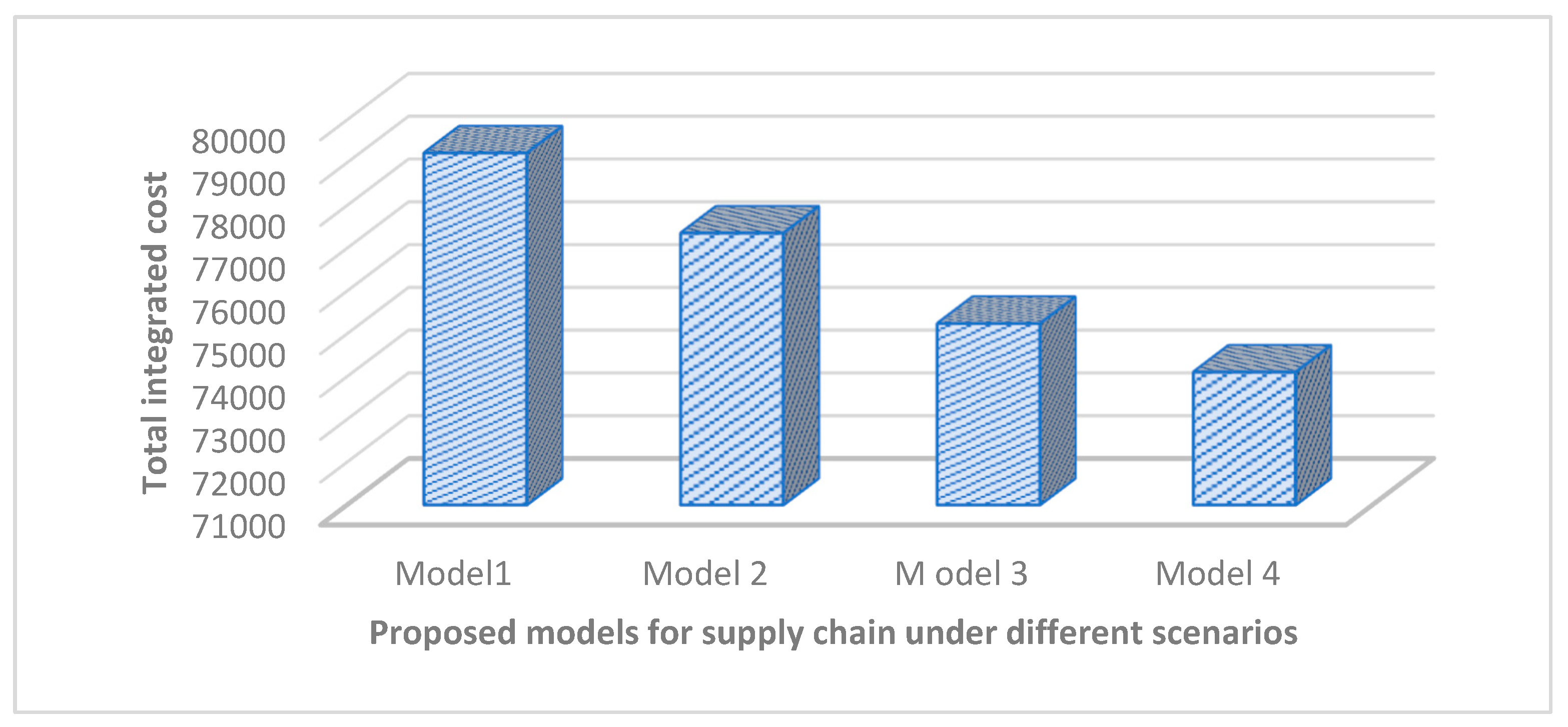
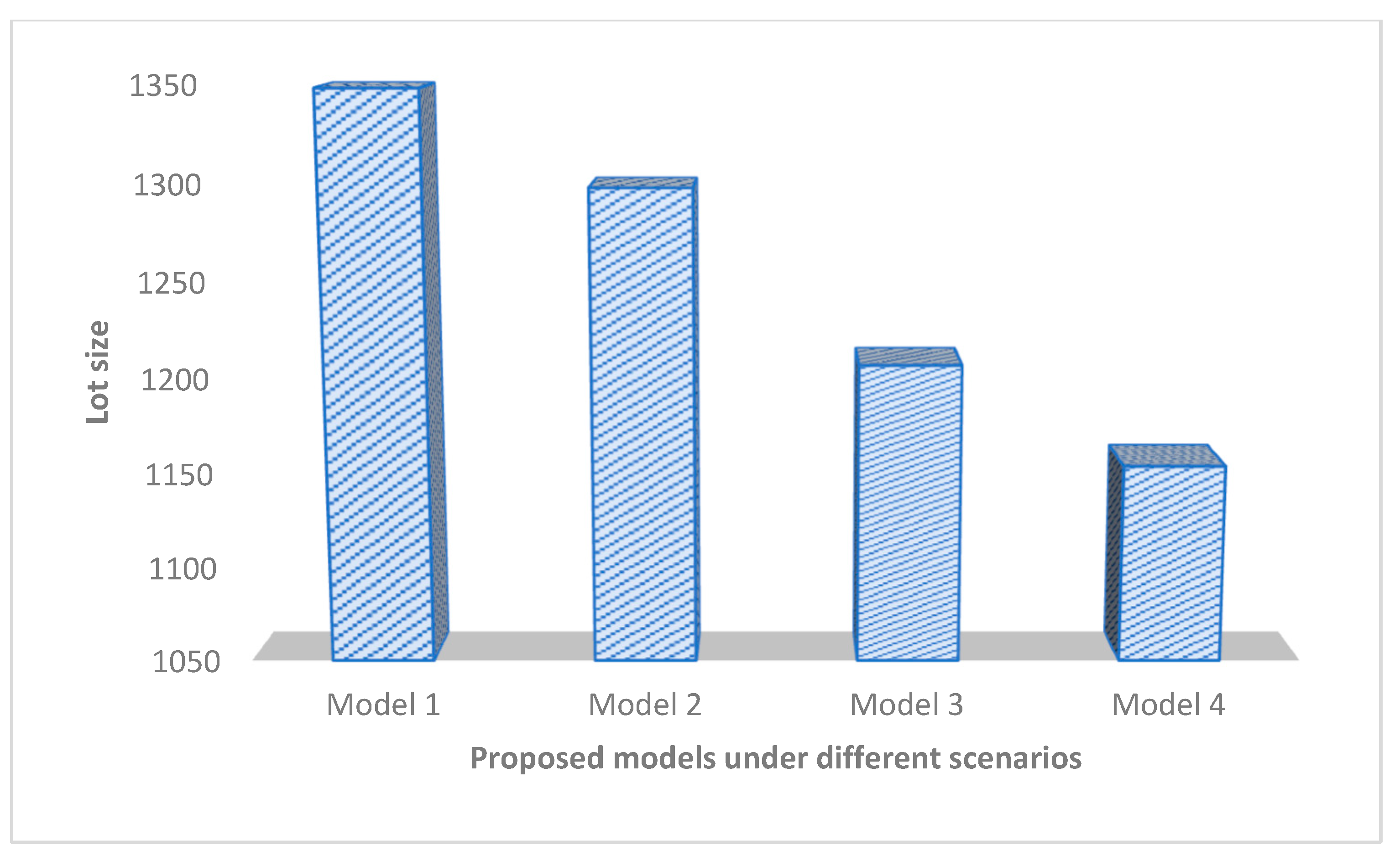
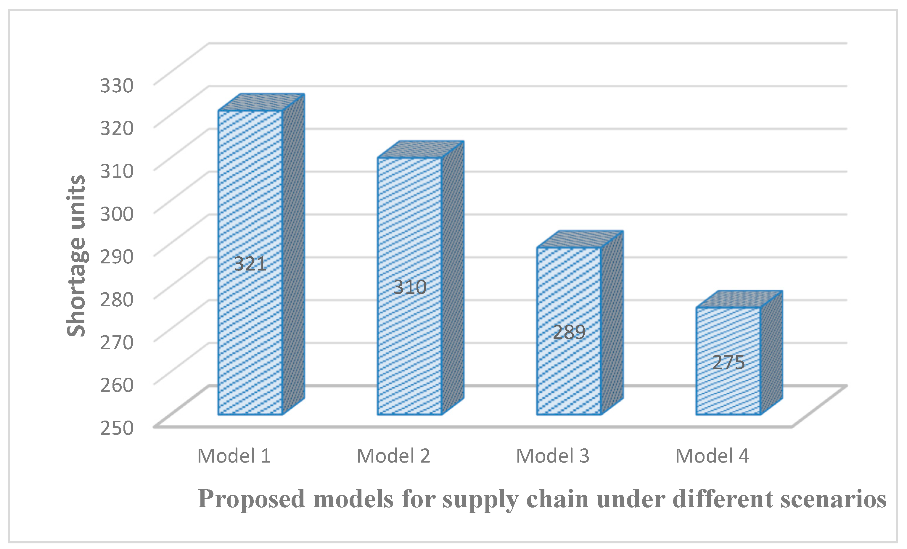
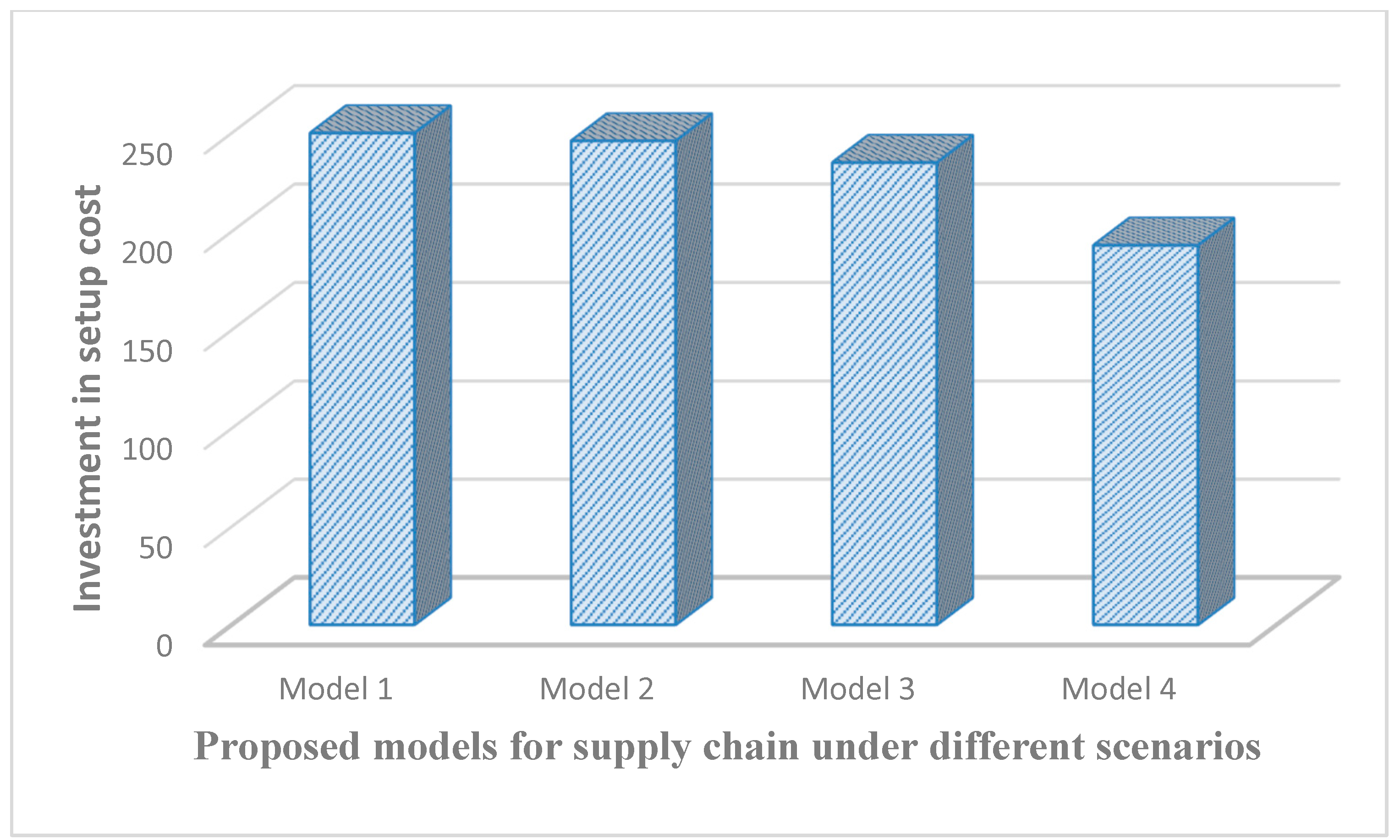
We replaced all known inventory parameters from Table 2 in Equation (37) and determined the optimality, algorithm and solution with the help of Mathematica software v12, and we obtained the values of the decision variables under proposed consideration. We provide four situations: (i) crisp model with waste management cost; (ii) the situation (i) improved with the fuzzy theory with the same assumption; (iii) the situation (ii) extended with the effect of learning in fuzzy environment; (iv) the situation (iii) extended with the cloudy fuzzy environment under a learning effect for the supply chain. In each situation, we calculated the decision variables. All the situations regarding this scenario are shown in Table 3 and also presented in Figure 10, Figure 11, Figure 12, Figure 13 and Figure 14.

5.14. Observation and Discussion of the Proposed Model

In this section, we present an analysis of our results in comparison to the contributions of others who performed nice work in this field.
We provide Table 4, in which selected authors’ contributions are given, and our contribution is given at the bottom of the Table 4.
From Table 3, it can be seen that the proposed model with learning in a cloudy fuzzy environment is more beneficial for the supply chain under the proposed assumptions because lot size, shipment, investment in setup, shortage units and total integrated fuzzy cost are more suitable for industries, firms and the business sector. We selected this scenario (model with learning in a cloudy fuzzy environment) for the sensitivity analysis of the model’s input inventory parameters for observations and managerial insights.

6. Sensitivity Analysis

Sensitivity analysis is the backbone of the industrial sector, firms and also many business sectors because the demand rate of the items, lot size, information about shortage units and inventory cost change the business direction. Supply chain members should be aware of such inventory decisions. This section covers the effects of the buyer’s holding cost, vendor’s holding cost, cloudy fuzzy demand rate, learning rate, percentage of defective items, vendor’s warranty cost and carbon emissions cost on the decision variable and total integrated fuzzy cost in the supply chain.

Observations and Managerial Insights

  • Impact of buyer’s holding cost
From Table 5, we determined that if the value of the buyer’s holding cost increases, then the number of shipments, shortages and total integrated fuzzy cost increase, but the lot size decreases. This means that the players in the supply chain should be more aware of the buyer’s holding cost because it affects the decision variables. It gives a positive response for the supply chain.
  • Impact of vendor’s holding cost
From Table 6, we determined that if the value of the vendor’s holding costs increases, then lot size, shortages and total integrated fuzzy cost increase, but the number of shipments decreases. The vendor’s holding cost also changes the decision variable and is also more sensitive regarding decision variables.
  • Impact of fixed transportation cost
From Table 7, we observed that if the value of fixed transportation increases, then lot size, shortages and total integrated fuzzy cost increase, but the shipment number decreases. The fixed transportation cost also changes the decision variable and also more sensitive parameters regarding decision variables in the supply chain.
  • Impact of fixed carbon emission cost
From Table 8, we observed that if the value of fixed carbon emission cost increases, then lot size, shortages and total integrated fuzzy cost increase, but the shipment number decreases. The fixed carbon emission cost also changes the decision variable and also more sensitive parameters regarding decision variables in the supply chain.
  • Impact of variable transportation cost
From Table 9, we can easily see that if the value of variable transportation cost increases, then lot size, shortages and shipment number are fixed, but the integrated fuzzy cost increases. The buyer and vendor both should be aware of these input parameters.
  • Impact of variable carbon emission cost
From Table 10, we can easily see that if the value of variable carbon emission cost increases, then lot size, shortages and shipment number are fixed, but the integrated fuzzy cost increases. The variable carbon emission cost has the same effect as the variable transportation cost.
  • Impact of setup cost reduction parameter
From Table 11, we observed that if the value of the setup cost reduction parameter increases, then lot size and shortages decrease, the shipment number is fixed and the integrated fuzzy cost increases; the investment in setup cost initially becomes zero, but when the setup cost reduction value is 0.0014, then the investment in setup cost is USD 193. This parameter is beneficial for a reduction in investment in setup cost; finally, it reduces the total integrated fuzzy cost in the supply chain.
  • Impact of learning rate
The learning rate affects the shipment, shortages, lot size and total integrated fuzzy cost. From Table 12, it can be seen that if the learning rate increases from 0.149 to 0.156, then the number of shipments, shortages and total integrated fuzzy cost decrease initially up to 0.152, whereas lot size increases, and after that, the number of shipments, shortages, lot size and total integrated fuzzy cost become constant.
  • Impact of cloudy demand parameters
From Table 13, it can be seen that if the values of the upper and lower deviations of the cloudy demand rate increase (ρ = 0.02 to 0.15 and σ = 0.01 to 0.13), then the number of shipments, lot size, shortages and total integrated fuzzy cost initially become constant, but when the values of cloudy parameters are ρ = 0.15 and σ = 0.13, then the number of shipments, lot size, shortages and total integrated fuzzy cost exhibit a minor decrease. A decision-maker should be aware of the values of the cloudy inputs.
  • Impact of upper and lower deviations of cloudy demand rate
From Table 14, it can be seen that if the values of the cloudy parameters increase ( H D = 10,000   t o   12,000   a n d   L D = 5000   t o   7000 ), then initially, the number of shipments, shortages and total integrated fuzzy cost increase, whereas lot size decreases. Market decision-makers should be aware of the values of the upper and lower deviations of the cloudy demand rate.
  • Impact of percentage of defectives
From Table 15, it can be seen that if the values of the percentage of defectives increase ( α = 0.04   t o   0.06 ) , then the number of shipments becomes constant, whereas shortages and total integrated fuzzy cost increase, but the lot size increases because the percentage of defective items increases in the lot.
  • Impact of unusable percentage of defectives
From Table 16, it can be seen that if the values of the unusable percentage of defectives increase ( δ = 0.01   t o   0.03 ) , then the number of shipments becomes constant, whereas shortages and total integrated fuzzy cost increase, but the lot size increases because the unstable percentage of defective items increases in the lot.

7. Concluding Remarks

7.1. Conclusions

The impact of education and carbon emissions on a comprehensive model of a green supply chain for faulty products in a fuzzy environment was examined in this article. Our research shows that a variety of sustainable supply chain models, in which a fuzzy triangle is used to illustrate the demand rate, would be beneficial to both sellers and buyers. We learned more about inventory parameters related to decision factors and joint total fuzzy profit from the management understanding and observations. Supply chain participants can benefit from this knowledge. In this approach, the learning idea plays a significant role in persuading the customer to place fewer, less frequent orders in order to increase profits. When demand is irregular, the seller will produce less since there may be greater risk involved in the transaction. By considering the seller’s and buyer’s strategies independently, a combined model has been created. The objective is to minimize the combined total fuzzy cost Ψ E C ( N * , M * , B * , μ * ) ) while concurrently optimizing the number of shipments ( N * ), order quantity value ( M * ), shortfall amount ( B * ) and investment in setup cost in a fuzzy environment with the influence of learning in a cloudy fuzzy environment. The developed model is also contrasted in Table 3 with and without learning in a fuzzy environment. The findings showed that demand deviation, or the rate at which the upper and lower deviations of the demand rate grow, leads to an increase in shipments and integrated total cloudy fuzzy cost but a drop in order quantity and shortfall units while other input parameters remain constant. The model’s feasibility is investigated using sensitivity analysis and numerical analysis. This study may be expanded to include credit financing policies and is applicable to the textile sector, several scientific laboratories and omnichannel marketing.

7.2. Limitation and Future Scope of Our Present Study

We speak about the limitations of our current paper in this part. Only supply chains where the rate of production rises and the rate of demand follows the triangle fuzzy number are included in our suggested model. It is likely to demonstrate a novel working theory. Researchers can look into additional novel waste management policies, warranty cost, investment in setup cost, setup cost reduction, carbon emission cost and learning in a cloudy fuzzy environment. The current analysis is predicated on supply chain inspections at the vendor and buyer ends. The impact of the buyer’s holding cost, vendor’s holding cost, learning rate, upper and lower deviations of demand rate, percentage of defectives, unusable defective percentage, investment in setup cost, waste management cost and different types of carbon emission costs and the value of their contributions to the supply chain under learning in a cloudy fuzzy environment may be analyzed by authors and the work of Aderohunmu and Mobolurin [77] can be improved by using of this theory.

7.3. Application of Our Present Study

Any product’s demand rate fluctuates over time and is often not fixed. From this vantage point, our research attempted to address the circumstance in which the demand rate is beginning to become inaccurate. The current study may be helpful in the context of an omnichannel environment where the buyer inspects the lot they received directly from the seller, the seller employs a product warranty policy, and the demand rate is unpredictable. One excellent illustration of our current approach is online purchasing on sites like Amazon, Flipkart and Snapdeal. A supply chain system between sellers, buyers, and clients is created by Amazon, Flipkart, Snapdeal and other businesses, and all participants occasionally make more money. Any product’s demand rate is often not set. From this vantage point, our research attempted to address the circumstance in which the demand rate is beginning to become inaccurate.

7.4. Research Limitations of Our Proposed Study

The limitations of the present paper are explained in this part. The present proposed model is a minimized integrated total cloudy fuzzy cost for a supply chain where the rate of demand follows a triangular fuzzy number. The lower and upper deviations of demand, learning input and costs also should be according to the proposed model; otherwise, the model cannot work well. The buyer’s holding cost, vendor’s holding cost, learning rate, carbon emission cost and percentage of defectives are effective input parameters, and their values are important for the seller and buyer points of view. The value of cloudy fuzzy parameters should be according to the proposed model, and then it will be beneficial for the seller and buyer; otherwise, the model will not work well.

7.5. Practical Implications and Future Scope

This study is very beneficial for supply chain management where builders want to earn more profit for a long time and want to more sales during the production of items. Nowadays, a lot of firms and business factories follow such types of policies, including Amazon, food factories and many other business companies. These companies inspect all items before delivery of the items to the clients or customers; if the clients/customers receive any scrap, damaged or otherwise unsatisfactory products, under the prescribed policy, there is a fixed return date, and a warranty policy with fixed EMI is also used.

7.6. Social Implications of Our Proposed Study

By using this proposed model, researchers and others can investigate new policies for managing waste and recovered items. The limitation of the model is that the inspection is performed at the vendor’s and buyer’s ends in the supply chain. The inspection process may have errors, and human error can be considered in an extended model. This model can be helpful for retailers, sellers or customers in cases where lots have some defective items and defective-quality items have been separated by using an inspection process. Examples include the manufacturing of toys, the supply of eggs and perishable items and fisheries.

7.7. Originality of Our Present Study

The originality of this proposed model is 100% because no part of it has been proposed or used in other business sectors. The demand rate for any product is not fixed in general; it varies with time. By considering this concept, we studied a supply chain model where the demand rate is imprecise in nature. The present work can be beneficial in the field of omnichannel environments where the demand rate is imprecise in nature and buyers use the strategy of trade credit policy and learning in a fuzzy environment. Online shopping is a good example of an area where this model can be applied.

Funding

This research received no external funding.

Data Availability Statement

Data are contained within the article.

Conflicts of Interest

The authors declare no conflict of interest.

References

  1. Salameh, M.K.; Jaber, M.Y. Economic production quantity model for items with imperfect quality. Int. J. Prod. Econ. 2000, 64, 59–64. [Google Scholar] [CrossRef]
  2. Biel, K.; Glock, C.H. Systematic literature review of decision support models for energy-efficient production planning. Comput. Ind. Eng. 2016, 101, 243–259. [Google Scholar] [CrossRef]
  3. Jaggi, C.K.; Mittal, M. Economic order quantity model for deteriorating items with imperfect quality. Int. J. Ind. Eng. Comput. 2011, 32, 107–113. [Google Scholar]
  4. Wee, H.M.; Yu, J.; Chen, M.C. Optimal inventory model for items with imperfect quality and shortage backordering. Omega 2007, 35, 7–11. [Google Scholar] [CrossRef]
  5. Eroglu, A.; Ozdemir, G. An economic order quantity model with defective items and shortages. Int. J. Prod. Econ. 2007, 106, 544–549. [Google Scholar] [CrossRef]
  6. Roy, M.D.; Sana, S.S.; Chaudhuri, K. An optimal shipment strategy for imperfect items in a stock-out situation. Math. Comput. Model. 2011, 54, 2528–2543. [Google Scholar] [CrossRef]
  7. Sarkar, B. Supply chain coordination with variable backorder, inspection and discount policy for fixed lifetime products. Math. Probl. Eng. 2016, 20, 1–14. [Google Scholar] [CrossRef]
  8. Jaggi, C.K.; Yadavalli, V.S.S.; Sharma, A.; Tiwari, S. A fuzzy EOQ model with allowable shortage under different trade credit terms. Appl. Math. Inf. Sci. 2016, 10, 785–805. [Google Scholar] [CrossRef]
  9. Sebatjane, M.; Adetunji, O. Economic order quantity model for growing items with imperfect quality. Oper. Res. Perspect. 2019, 6, 100088. [Google Scholar] [CrossRef]
  10. Öztürk, H. A deterministic production inventory model with defective items, imperfect rework process and shortages backordered. Int. J. Oper. Res. 2020, 39, 237–261. [Google Scholar] [CrossRef]
  11. Gautam, P.; Khanna, A.; Jaggi, C.K. An integrated green supply chain model with product recovery management towards a cleaner system. J. Clean. Prod. 2021, 320, 128850. [Google Scholar] [CrossRef]
  12. Jayaswal, M.K.; Mittal, M. Learning-based inventory model for deteriorating imperfect quality items under inflation. Int. J. Manag. Pract. 2022, 15, 429–444. [Google Scholar] [CrossRef]
  13. Narang, P.; De, P.K. An imperfect production-inventory model for reworked items with advertisement, time and price dependent demand for non-instantaneous deteriorating item using genetic algorithm. Int. J. Math. Oper. Res. 2023, 24, 53–77. [Google Scholar] [CrossRef]
  14. Taleizadeh, A.A.; Naghavi-Alhoseiny, M.S.; Cárdenas-Barrón, L.E.; Amjadian, A. Optimization of price, lot size and backordered level in an EPQ inventory model with rework process. RAIRO-Oper. Res. 2024, 58, 803–819. [Google Scholar] [CrossRef]
  15. Tang, S.; Wang, W.; Yan, H.; Hao, G. Low carbon logistics: Reducing shipment frequency to cut carbon emissions. Int. J. Prod. Econ. 2015, 164, 339–350. [Google Scholar] [CrossRef]
  16. Wang, Q.; Wu, J.; Zhao, N.; Zhu, Q. Inventory control and supply chain management: A green growth perspective. Resour. Conserv. Recycl. 2019, 145, 78–85. [Google Scholar] [CrossRef]
  17. Zhu, L.; Zhou, J.; Yu, Y.; Zhu, J. Emission-dependent production for environment aware demand in cap-and-trade system. J. Adv. Manuf. Syst. 2017, 16, 67–80. [Google Scholar] [CrossRef]
  18. Zhang, X.; Liu, P.; Li, Z.; Yu, H. Modeling the effects of low-carbon emission constraints on mode and route choices in transportation networks. Procedia-Soc. Behav. Sci. 2013, 96, 329–338. [Google Scholar] [CrossRef]
  19. Sarkar, B.; Ganguly, B.; Sarkar, M.; Pareek, S. Effect of variable transportation and carbon emission in a three-echelon supply chain model. Transp. Res. Part E Logist. Transp. Rev. 2016, 91, 112–128. [Google Scholar] [CrossRef]
  20. Tiwari, S.; Daryanto, Y.; Wee, H.M. Sustainable inventory management with deteriorating and imperfect quality items considering carbon emission. J. Clean. Prod. 2018, 192, 281–292. [Google Scholar] [CrossRef]
  21. Gautam, P.; Khanna, A. An imperfect production inventory model with setup cost reduction and carbon emission for an integrated supply chain. Uncertain Supply Chain. Manag. 2018, 6, 271–286. [Google Scholar] [CrossRef]
  22. Thomas, A.; Mishra, U. A sustainable circular economic supply chain system with waste minimization using 3D printing and emissions reduction in plastic reforming industry. J. Clean. Prod. 2022, 345, 131128. [Google Scholar] [CrossRef]
  23. Sharma, N.; Jain, M.; Sharma, D. ANFIS and metaheuristic optimization for green supply chain with inspection and rework. arXiv 2024, arXiv:2401.09154. [Google Scholar]
  24. Nobil, E.; Cárdenas-Barrón, L.E.; Garza-Núñez, D.; Treviño-Garza, G.; Céspedes-Mota, A.; de Jesús Loera-Hernández, I.; Nobil, A.H. Sustainability inventory management model with warm-up process and shortage. Oper. Res. Perspect. 2024, 12, 100297. [Google Scholar] [CrossRef]
  25. Ruidas, S.; Seikh, M.R.; Nayak, P. K A production inventory model with interval-valued carbon emission parameters under price-sensitive demand. Compu. Ind. Eng. 2021, 154, 107154. [Google Scholar] [CrossRef]
  26. Jaber, M.Y.; Goyal, S.K.; Imran, M. Economic production quantity model for items with imperfect quality subject to learning effects. Int. J. Prod. Econ. 2008, 115, 143–150. [Google Scholar] [CrossRef]
  27. Khan, M.; Jaber, M.Y.; Wahab, M.I.M. Economic order quantity model for items with imperfect quality with learning in inspection. Int. J. Prod. Econ. 2010, 124, 87–96. [Google Scholar] [CrossRef]
  28. Bazan, E.; Jaber, M.Y.; Zanoni, S. Supply chain models with greenhouse gases emissions, energy usage and different coordination decisions. Appl. Math. Model. 2015, 39, 5131–5151. [Google Scholar] [CrossRef]
  29. Sahoo, S.; Acharya, M.; Patnaik, S. Sustainable intuitionistic fuzzy inventory models with preservation technology investment and shortages. Int. J. Reason.-Based Intell. Syst. 2022, 14, 8–18. [Google Scholar] [CrossRef]
  30. Rajput, N.; Pandey, R.K.; Chauhan, A. Fuzzy optimization of a Production Model with CNTFN Demand Rate under Trade-Credit Policy. IJMOR 2022, 21, 200–220. [Google Scholar] [CrossRef]
  31. Gautam, P.; Kishore, A.; Khanna, A.; Jaggi, C.K. Strategic defect management for a sustainable green supply chain. J. Clean. Prod. 2019, 233, 226–241. [Google Scholar] [CrossRef]
  32. Jamal, A.M.M.; Sarker, B.R.; Wang, S. An ordering policy for deteriorating items with allowable shortage and permissible delay in payment. J. Oper. Res. Soc. 1997, 48, 826–833. [Google Scholar] [CrossRef]
  33. Rout, C.; Paul, A.; Kumar, R.S.; Chakraborty, D.; Goswami, A. Integrated optimization of inventory, replenishment and vehicle routing for a sustainable supply chain under carbon emission regulations. J. Clean. Prod. 2021, 316, 128256. [Google Scholar] [CrossRef]
  34. Singh, A.; Goel, A. Design of the supply chain network for the management of textile waste using a reverse logistics model under inflation. Energy 2024, 292, 130615. [Google Scholar] [CrossRef]
  35. Maity, S.; Chakraborty, A.; De, S.K.; Pal, M. A study of an EOQ model of green items with the effect of carbon emission under pentagonal intuitionistic dense fuzzy environment. Soft. Comput. 2023, 27, 15033–15055. [Google Scholar] [CrossRef]
  36. Jaber, M.Y.; Bonney, M. Optimal lot sizing under learning considerations: The bounded learning case. Appl. Math. Model. 1996, 20, 750–755. [Google Scholar] [CrossRef]
  37. Marchi, B.; Zanoni, S.; Zavanella, L.E.; Jaber, M.Y. Supply chain models with greenhouse gases emissions, energy usage, imperfect process under different coordination decisions. Int. J. Prod. Econ. 2019, 211, 145–153. [Google Scholar] [CrossRef]
  38. Chu, P.; Chung, K.J.; Lan, S.P. Economic order quantity of deteriorating items under permissible delay in payments. Comput. Oper. Res. 1998, 25, 817–824. [Google Scholar] [CrossRef]
  39. Pal, B.; Sana, S.S.; Chaudhuri, K. Three-layer supply chain–a production-inventory model for reworkable items. Appl. Math. Comput. 2012, 219, 530–543. [Google Scholar] [CrossRef]
  40. Giri, B.C.; Masanta, M. Developing a closed-loop supply chain model with price and quality dependent demand and learning in production in a stochastic environment. Int. J. Syst. Sci. Oper. Logist. 2020, 7, 147–163. [Google Scholar] [CrossRef]
  41. Alamri, O.A.; Jayaswal, M.K.; Khan, F.A.; Mittal, M. An EOQ Model with Carbon Emissions and Inflation for Deteriorating Imperfect Quality Items under Learning Effect. Sustainability 2022, 14, 1365. [Google Scholar] [CrossRef]
  42. Sangal, I.; Agarwal, A.; Rani, S. A fuzzy environment inventory model with partial backlogging under learning effect. Int. J. Comput. Appl. 2016, 137, 25–32. [Google Scholar] [CrossRef]
  43. Jaggi, C.K.; Pareek, S.; Goel, S.K.; Nidhi. An inventory model for deteriorating items with ramp type demand under fuzzy environment. Int. J. Logist. Syst. Manag. 2015, 22, 436–463. [Google Scholar] [CrossRef]
  44. Jaggi, C.K.; Sharma, A.; Jain, R. EOQ model with permissible delay in payments under fuzzy environment. In Analytical Approaches to Strategic Decision-Making: Interdisciplinary Considerations; IGI Global: Hershey, PA, USA, 2014; pp. 281–296. [Google Scholar]
  45. Sharma, L.K.; Vishal, V.; Singh, T.N. Developing novel models using neural networks and fuzzy systems for the prediction of strength of rocks from key geomechanical properties. Measurement 2017, 102, 158–169. [Google Scholar] [CrossRef]
  46. Patro, R.; Acharya, M.; Nayak, M.M.; Patnaik, S. A fuzzy EOQ model for deteriorating items with imperfect quality using proportionate discount under learning effects. Int. J. Manag. Decis. Mak. 2018, 17, 171–198. [Google Scholar] [CrossRef]
  47. Bhavani, G.D.; Meidute-Kavaliauskiene, I.; Mahapatra, G.S.; Činčikaitė, R. A Sustainable Green Inventory System with Novel Eco-Friendly Demand Incorporating Partial Backlogging under Fuzziness. Sustainability 2022, 14, 9155. [Google Scholar] [CrossRef]
  48. Jayaswal, M.K.; Mittal, M.; Alamri, O.A.; Khan, F.A. Learning EOQ model with trade-credit financing policy for imperfect quality items under cloudy fuzzy environment. Mathematics 2022, 10, 246. [Google Scholar] [CrossRef]
  49. Alamri, O.A. Sustainable Supply Chain Model for Defective Growing Items (Fishery) with Trade Credit Policy and Fuzzy Learning Effect. Axioms 2023, 12, 436. [Google Scholar] [CrossRef]
  50. Alsaedi, B.S.; Alamri, O.A.; Jayaswal, M.K.; Mittal, M. A sustainable green supply chain model with carbon emissions for defective items under learning in a fuzzy environment. Mathematics 2023, 11, 301. [Google Scholar] [CrossRef]
  51. Padiyar, S.S.; Bhagat, N.; Singh, S.R.; Punetha, N.; Dem, H. Production policy for an integrated inventory system under cloudy fuzzy environment. Int. J. Appl. Decis. Sci. 2023, 16, 255–299. [Google Scholar]
  52. Mahata, G.C.; De, S.K.; Bhattacharya, K.; Maity, S. Three-echelon supply chain model in an imperfect production system with inspection error, learning effect, and return policy under fuzzy environment. Int. J. Syst. Sci. Oper. Logist. 2023, 10, 1962427. [Google Scholar] [CrossRef]
  53. Sugapriya, C.; Saranyaa, P.; Nagarajan, D.; Pamucar, D. Triangular intuitionistic fuzzy number based backorder and lost sale in production, remanufacturing and inspection process. Expert Syst. Appl. 2024, 240, 122261. [Google Scholar] [CrossRef]
  54. Garg, H.; Sugapriya, C.; Rajeswari, S.; Nagarajan, D.; Alburaikan, A. A model for returnable container inventory with restoring strategy using the triangular fuzzy numbers. Soft Comput. 2024, 28, 2811–2822. [Google Scholar] [CrossRef]
  55. Shah, H.; Patel, M. An EOQ model for deteriorating items when demand is cloud fuzzy. Int. J. Logist. Syst. Manag. 2021, 42, 140–152. [Google Scholar] [CrossRef]
  56. De, S.K.; Mahata, G.C. A cloudy fuzzy economic order quantity model for imperfect-quality items with allowable proportionate discounts. J. Ind. Eng. Int. 2019, 15, 571–583. [Google Scholar] [CrossRef]
  57. Dubois, D.; Prade, H. Fuzzy Sets and Systems: Theory and Applications; Academic Press: New York, NY, USA, 1980. [Google Scholar]
  58. Turk, S.; Ozcan, E.; John, R. Multi-objective optimization in inventory planning with supplier selection. Expert Syst. Appl. 2017, 78, 51–63. [Google Scholar] [CrossRef]
  59. Wu, K.S.; Ouyang, L.Y. 2003. An integrated single-vendor single-buyer inventory system with shortage derived algebraically. Prod. Plann. Contr. 2003, 14, 555–561. [Google Scholar] [CrossRef]
  60. Masanta, M.; Giri, B.C. A closed-loop supply chain model with learning effect, random return and imperfect inspection underprice-and quality-dependent demand. Opsearch 2022, 59, 1094–1115. [Google Scholar] [CrossRef]
  61. Xu, J.; Chen, Y.; Bai, Q. A two-echelon sustainable supply chain coordination under cap-and-trade regulation. J. Clean. Prod. 2016, 135, 42–56. [Google Scholar] [CrossRef]
  62. Das, S.; Shaikh, A.A.; Bhunia, A.K.; Konstantaras, I. Warranty, free service and rework policy for an imperfect manufacturing system with SAR sensitive demand under emission taxation. Comput. Ind. Eng. 2024, 187, 109765. [Google Scholar] [CrossRef]
  63. Kazemi, N.; Shekarian, E.; Cárdenas-Barrón, L.E.; Olugu, E.U. Incorporating human learning into a fuzzy EOQ inventory model with backorders. Comput. Ind. Eng. 2015, 87, 540–542. [Google Scholar] [CrossRef]
  64. Björk, K.M. An analytical solution to a fuzzy economic order quantity problem. Int. J. Approx. Reason. 2009, 50, 485–493. [Google Scholar] [CrossRef]
  65. Wright, T.P. Factors affecting the cost of airplanes. J. Aeronaut. Sci. 1936, 3, 122–128. [Google Scholar] [CrossRef]
  66. Hsu, J.T.; Hsu, L.F. An integrated vendor-buyer cooperative inventory model for items with imperfect quality and shortage backordering. Adv. Decis. Sci. 2013, 65, 493–505. [Google Scholar] [CrossRef]
  67. Chang, H.C. An application of fuzzy sets theory to the EOQ model with imperfect quality items. Comp. Comput. Oper. Res. 2004, 31, 2079–2092. [Google Scholar] [CrossRef]
  68. Yu, J.C.; Wee, H.M.; Chen, J.M. Optimal ordering policy for a deteriorating item with imperfect quality and partial backordering. J. Chin. Inst. Ind. Eng. 2005, 22, 509–520. [Google Scholar] [CrossRef]
  69. Chung, K.J.; Huang, Y.F. Retailer’s optimal cycle times in the EOQ model with imperfect quality and a permissible credit period. Qual. Quant. 2006, 40, 59–77. [Google Scholar] [CrossRef]
  70. Konstantaras, I.; Skouri, K.; Jaber, M.Y. Inventory models for imperfect quality items with shortages and learning in inspection. Appl. Math. Model. 2012, 36, 5334–5343. [Google Scholar] [CrossRef]
  71. Sulak, H. An EOQ model with defective items and shortages in fuzzy sets environment. Int. J. Soc. Sci. Educ. Res. 2015, 2, 915–929. [Google Scholar] [CrossRef]
  72. Shekarian, E.; Olugu, E.U.; Abdul-Rashid, S.H.; Kazemi, N. An economic order quantity model considering different holding costs for imperfect quality items subject to fuzziness and learning. J. Intell. Fuzzy Syst. 2016, 30, 2985–2997. [Google Scholar] [CrossRef]
  73. Khanna, A.; Gautam, P.; Jaggi, C.K. Inventory modeling for deteriorating imperfect quality items with selling price dependent demand and shortage backordering under credit financing. Int. J. Math. Eng. Manag. Sci. 2017, 2, 110. [Google Scholar] [CrossRef]
  74. Rajeswari, S.; Sugapriya, C. Fuzzy economic order quantity model with imperfect quality items under repair option. J. Res. Lepidoptera 2020, 51, 627–643. [Google Scholar]
  75. Tahami, H.; Fakhravar, H. A fuzzy inventory model considering imperfect quality items with receiving reparative batch and order. Eur. J. Engin. Tech. Res. 2020, 5, 1179–1185. [Google Scholar]
  76. Jayaswal, M.K.; Mittal, M.; Sangal, I. Ordering policies for deteriorating imperfect quality items with trade-credit financing under learning effect. Int. J. Syst. Assur. Eng. Manag. 2021, 12, 112–125. [Google Scholar] [CrossRef]
  77. Aderohunmu, R.; Mobolurin, A.; Bryson, N. Joint vendor-buyer policy in JIT manufacturing. J. Oper. Res. Soc. 1995, 46, 375–385. [Google Scholar] [CrossRef]
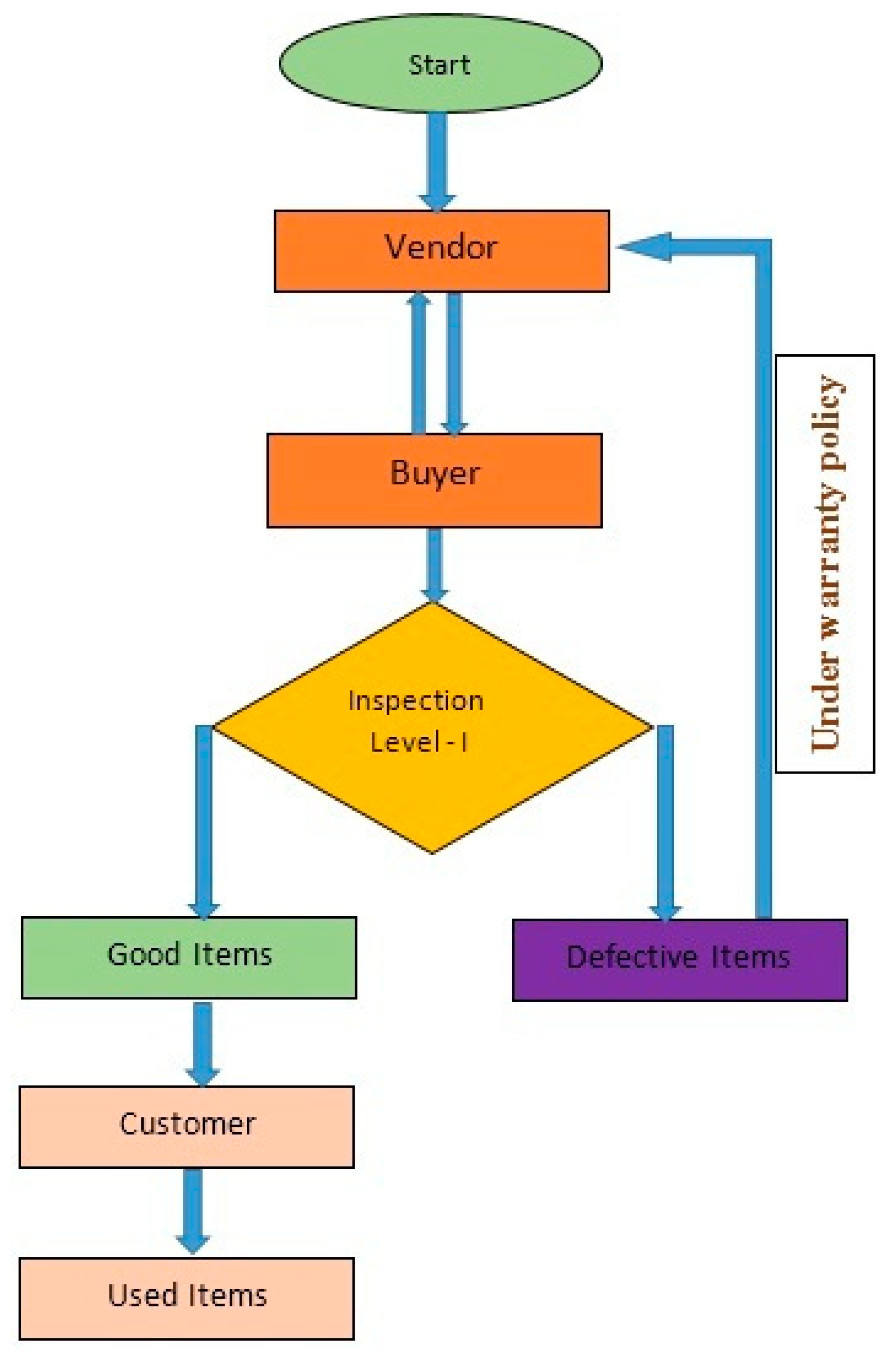
Figure 1. The buyer and seller plans in the supply chain.
Mathematics 12 01603 g001
Figure 2. The working plan of the present model in a supply chain through a flowchart.
Mathematics 12 01603 g002
Figure 3. Membership function of a triangular fuzzy number.
Mathematics 12 01603 g003
Figure 4. Representation of cloudy normalized triangular fuzzy number (CNTFN).
Mathematics 12 01603 g004
Figure 5. Wright’s curve.
Mathematics 12 01603 g005
Figure 6. Representation of vendor’s scenario over time.
Mathematics 12 01603 g006
Figure 7. Representation of vendor’s policy scenario over time.
Mathematics 12 01603 g007
Figure 8. Representation of vendor’s holding cost.
Mathematics 12 01603 g008
Figure 9. Representation of buyer’s inventory system over time.
Mathematics 12 01603 g009
Figure 10. Discussion of total integrated cost for the supply chain under different models.
Mathematics 12 01603 g010
Figure 11. Discussion of lot size for the supply chain under different models.
Mathematics 12 01603 g011
Figure 12. Discussion of shortage units for the supply chain under different models.
Mathematics 12 01603 g012
Figure 13. Discussion of investment in setup cost for the supply chain under different models.
Mathematics 12 01603 g013
Figure 14. Discussion of shipments for the supply chain under different models.
Mathematics 12 01603 g014
Table 1. Authors’ contribution and our proposed contribution.
Authors’ Contribution Imperfect ItemsSupply ChainWaste Management CostSetup Cost Reduction Policy Warranty Policy Carbon Emissions Cloudy Fuzzy Environment Learning in Cloudy Fuzzy
Shah and Patel [55]
De and Mahata [56]
Dubois and Prade [57]
Salameh and Jaber [1]
Turk et al. [58]
Wu et al. [59]
Jayaswal et al. [48]
Masanta and Giri [60]
Xu et al. [61]
Padiyar et al. [51]
Mahata et al. [52]
Das et al. [62]
Singh and Goel [34]
Current study
Table 2. Model’s inventory input parameters.
Input ParametersNumerical Values Input ParametersNumerical Values
W 160,000 units per year D 50,000 units per year
K USD 300 per order F T USD 25 per order
V T USD 0.1 per unit F C USD 5 per delivery
V c USD 5 per unit C b USD 10 per unit per unit
S b USD 0.5 per unit h 1 USD 2 per unit per year
h 2 USD 3 per unit per year k 1 USD 200 per order
k 2 USD 100 per order s 0.79
h v USD 2 per unit ω v USD 30 per unit
A v USD 1000 per setup π USD 0.00140
E [ α ] 0.04% E [ δ ] 0.01%
H D 10,000 units per year L D 5000 units per year
σ 0.15 ρ 0.13
L v USD 0.5 per unusable item i 2
Table 3. Proposed model with optimal solution (decision variables) for supply chain under various models.
Decision   Variable s
Model  
Shipment
N *
Order
Quantity
M N *
Shortage Units
B N *
Investment   in   Setup   ( USD )   μ * Total Integrated Inventory Cost (USD)
Ψ E C N * , M N * , B N * , μ *
Crisp model with waste management cost111348.75321.6725079,228.87
Model with fuzzy
environment
91298.74310.9824677,354.97
Model with learning in fuzzy environment with learning rate 0.15261207.11289.6523575,241.98
Model with learning in cloudy fuzzy environment with learning rate 0.15251154.56275.9819374,105.85
Table 4. Comparison of results with our proposed model.
AuthorsInvestment in Setup
as a Decision Variable
Lot Size
as a Decision Variable
Shortage Units
as a Decision Variable
Shipment
as a Decision Variable
Total Profit/
Total Cost EOQ/EPQ/Supply Chain
Salsmeh and Jaber [1]Not calculated1439 units-Not calculatedUSD 1,212,235
Chang [67]Not calculated1429 units-Not calculatedUSD 121,366.72
Yu et al. [68]Not calculated1288 units28 unitsNot calculatedUSD 1,212,148
Chung and Huang [69]Not calculated196 units Not calculatedUSD 346,583.3
Eroglu and Ozdemir [5]Not calculated2129 units595 unitsNot calculatedUSD 341,116.89
Jaber et al. [27]Not calculated1440 units-Not calculatedUSD 1,217,452
Khan et al. [35]Not calculated2201 units2112 unitsNot calculatedUSD 1,222,394
Jaggi and Mittal [18]Not calculated1283 units-Not calculatedUSD 1,224,183
Konstantaras et al. [70]Not calculated666 units-Not calculatedUSD 68,985
Jaggi et al. [43]Not calculated1642 units674 unitsNot calculatedUSD 347,086
Sulak [71]Not calculated2149 units594.53Not calculatedUSD 341,121.2
Shekarian et al. [72]Not calculated5000 units Not calculatedUSD 11,000,000
Khanna et al. [73]Not calculated899 units283 unitsNot calculatedUSD 707,837
Patro et al. [46]Not calculated1117 units Not calculatedUSD 1,273,420
Jayaswal et al. [48]Not calculated1336 units-Not calculatedUSD 1,206,930
Rajeswari and Sugapriya [74]Not calculated3423 units-Not calculatedUSD 1,197,300
Tahami and Fakhravar [75]Not calculated1295 units-Not calculatedUSD 1,212,072
Jayaswal et al. [76]Not calculated3756 units-Not calculatedUSD 1,142,850
Alamri et al. [49]Not calculated48,225 units-Not calculatedUSD 1,662,440
Our paper under supply chainCalculated, USD 1931154 units275.98 unitsCalculated, 5Total inventory fuzzy cost for the supply chain USD 74,105.85
Table 5. Variable impact of buyer’s holding cost on N * ,   M N * ,   B N * and Ψ E C (USD); the rest of the inventory parameters are fixed.
Buyer’s Holding Cost
hb
Shipment
N*
Lot Size
M(N*)
Stortage Units
B(N*)
Total Integrated Fuzzy Cost
Ψ EC(USD)
2.5021406.87228.1873,805.15
3.7531218.76245.2373,905.45
5.0051154.56275.9874,105.85
Table 6. Variable impact of vendor’s holding cost on N * ,   M N * ,   B N * and Ψ E C (USD); the rest of the inventory parameters are fixed.
Vendor’s Holding Cost
hv
Shipment
N*
Lot Size
M(N*)
Stortage Units
B(N*)
Total Integrated Fuzzy Cost
Ψ EC(USD)
1.009992.32254.1873,874.65
3.0071098.76265.2373,986.89
5.0051154.56275.9874,105.85
Table 7. Variable impact of fixed transportation cost on N * ,   M N * ,   B N * and Ψ E C (USD); the rest of the inventory parameters are fixed.
Fixed Transportation Cost FT Shipment
N*
Lot Size
M(N*)
Stortage Units
B(N*)
Total Integrated Fuzzy Cost
Ψ EC(USD)
12.0010997.54203.5273,898.31
18.0081088.32255.8173,903.43
25.0051154.56275.9874,105.85
Table 8. Variable impact of fixed carbon emission cost on N * ,   M N * ,   B N * and Ψ E C (USD); the rest of the inventory parameters are fixed.
Fixed Carbon Emission Cost Fc Shipment
N*
Lot Size
M(N*)
Stortage Units
B(N*)
Total Integrated Fuzzy Cost
Ψ EC(USD)
2.5091087.54252.5273,798.17
3.7581098.65261.8173,898.51
5.0051154.56275.9874,105.85
Table 9. Variable impact of variable transportation cost on N * ,   M N * ,   B N * and Ψ E C (USD); the rest of the inventory parameters are fixed.
Variable Transportation Cost VT Shipment
N*
Lot Size
M(N*)
Stortage Units
B(N*)
Total Integrated Fuzzy Cost Ψ EC(USD)
0.05051154.56275.9874,070.97
0.07551154.56275.9874,065.87
0.10051154.56275.9874,105.85
Table 10. Variable impact of variable carbon emission cost on N * ,   M N * ,   B N * and Ψ E C (USD); the rest of the inventory parameters are fixed.
Variable Carbon Emission Cost Vc Shipment
N*
Lot Size
M(N*)
Stortage Units
B(N*)
Total Integrated Fuzzy Cost Ψ EC(USD)
2.5051154.56275.9873,170.1
3.7551154.56275.9873,265.87
5.0051154.56275.9874,105.85
Table 11. Variable impact of setup cost reduction on N * ,   M N * ,   B N * and Ψ E C (USD); the rest of the inventory parameters are fixed.
Setup Cost Reduction Input Parameter Cost π Shipment
N*
Lot Size
M(N*)
Stortage Units
B(N*)
Investment in Setup Cost
(μ*)
Total Integrated
Fuzzy Cost
Ψ EC(USD)
0.000751159.65278.09074,145.10
0.001051159.45279.780.00000174,135.87
0.001451154.56275.98193.6574,105.85
Table 12. Variable impact of learning rate on N * ,   M N * ,   B N * and Ψ E C (USD); the rest of the inventory parameters are fixed.
Learning Rate l Shipment
N*
Lot Size
M(N*)
Stortage Units
B(N*)
Total Integrated
Fuzzy Cost Ψ EC(USD)
0.14910985.65289.0975,798.09
0.15081062.17281.7874,835.92
0.15251154.56275.9874,105.85
0.15451154.56275.9874,105.85
0.15651154.56275.9874,105.85
Table 13. Variable impact of cloudy fuzzy parameters on N * , M N * ,   B N * and Ψ E C (USD); the rest of the inventory parameters are fixed.
Cloud
Parameter ρ (0 < ρ < 0)
Cloud Parameter
σ (0 < σ < 0)
Shipment
N*
Lot Size
M(N*)
Stortage Units
B(N*)
Total Integrated
Fuzzy Cost
Ψ EC(USD)
0.020.0181174.56278.9874,110.12
0.030.0281174.56278.9874,110.12
0.040.0381174.56278.9874,110.12
0.050.0481174.56278.9874,110.12
0.060.0581174.56278.9874,110.12
0.090.0881174.56278.9874,110.12
0.150.1351154.56275.9874,105.85
Table 14. Variable impact of upper and lower deviations of demand rate on N * ,   M N * ,   B N * and Ψ E C (USD); the rest of the inventory parameters are fixed.
Upper Deviation
of Demand Rate Δ H D
Lower Deviation
of Demand Rate Δ L D
Shipment
N*
Lot Size
M(N*)
Stortage Units
B(N*)
Total Integrated
Fuzzy Cost
Ψ EC(USD)
10,000500051174.56278.9874,105.85
11,000600071103.56288.9874,144.97
12,000700061087.56292.9874,198.65
Table 15. Variable impact of percentage of defectives on N * ,   M N * ,   B N * and Ψ E C (USD); the rest of the inventory parameters are fixed.
Percentage of Defectives α Shipment
N*
Lot Size
M(N*)
Stortage Units
B(N*)
Total Integrated
Fuzzy Cost
Ψ EC(USD)
0.0451154.56275.9874,105.85
0.0551159.71265.7874,980.13
0.0651164.41256.9875,210.08
Table 16. Variable impact of unusable percentage of defectives on N * ,   M N * ,   B N * and Ψ E C (USD); the rest of the inventory parameters are fixed.
Waste Percentage of Unusable Products δ Shipment
N*
Lot Size
M(N*)
Stortage Units
B(N*)
Total Integrated
Fuzzy Cost
Ψ EC(USD)
0.0151154.56275.9874,105.85
0.0251156.01271.0774,117.13
0.0351157.05273.0875,119.08
Disclaimer/Publisher’s Note: The statements, opinions and data contained in all publications are solely those of the individual author(s) and contributor(s) and not of MDPI and/or the editor(s). MDPI and/or the editor(s) disclaim responsibility for any injury to people or property resulting from any ideas, methods, instructions or products referred to in the content.