Article

Dynamics of a Model of Coronavirus Disease with Fear Effect, Treatment Function, and Variable Recovery Rate

by
Rubayyi T. Alqahtani
1,*,
Abdelhamid Ajbar
2 and
Nadiyah Hussain Alharthi
1
1
Department of Mathematics and Statistics, College of Science, Imam Mohammad Ibn Saud Islamic University (IMSIU), Riyadh 13318, Saudi Arabia
2
Department of Chemical Engineering, King Saud University, Riyadh 11362, Saudi Arabia
*
Author to whom correspondence should be addressed.
Mathematics 2024, 12(11), 1678; https://doi.org/10.3390/math12111678
Submission received: 11 March 2024 / Revised: 2 May 2024 / Accepted: 21 May 2024 / Published: 28 May 2024
(This article belongs to the Section Computational and Applied Mathematics)

Abstract

:
In this work, we developed, validated, and analysed the behaviour of a compartmental model of COVID-19 transmission in Saudi Arabia. The population was structured into four classes: susceptible (S), exposed (E), infectious (I), and removed (R) individuals. This SEIR model assumes a bilinear incidence rate and a nonlinear recovery rate that depends on the quality of health services. The model also considers a treatment function and incorporates the effect of fear due to the disease. We derived the expression of the basic reproduction number and the equilibrium points of the model and demonstrated that when the reproduction number is less than one, the disease-free equilibrium is stable, and the model predicts a backward bifurcation. We further found that when the reproduction number is larger than one, the model predicts stable periodic behaviour. Finally, we used numerical simulations with parameter values fitted to Saudi Arabia to analyse the effects of the model parameters on the model-predicted dynamic behaviours.

1. Introduction

Although the COVID-19 pandemic appears to have ended, numerous lessons can still be learned from it. Ample data related to the pandemic are available, and research on this topic—particularly on the modelling and understanding of the factors that affected the disease dynamics—is still underway [1,2,3,4]. Mathematical models played a crucial role at the beginning of the pandemic, predicting disease transmission and providing public health authorities with guidance on the effectiveness of mitigation and control measures, such as quarantine [5], media coverage [6], lockdowns [7], and travel restrictions [8].
Many types of mathematical models have been proposed in the literature since the start of the pandemic. An overview, although non-exhaustive, of the multitude of modelling frameworks was provided in [9,10]. These include models based on logistic Equations [11], compartmental epidemic models (e.g., SIR and SEIR) [1,2,3,12], models based on statistical techniques [13], models based on fractional-order derivatives [14] and Caputo derivatives [15], and artificial neural networks [16]. Despite their relative simplicity, compartmental epidemic models with various structures are still widely used to model infectious diseases, including COVID-19 [1,2,3,17]. The models’ variable structures allow different segments of the affected populations (such as individuals who are quarantined, re-infected, and hospitalised) to be incorporated, and they can include different expressions of the incidence rate [18].
In this paper, we propose and study a simple, yet practical model, for COVID-19 transmission. The study population was divided into four segments: susceptible (S), exposed (E), infectious (I), and removed (recovered or deceased) (R) individuals. We validated the model with COVID-19 data from Saudi Arabia.
One key element in modelling the spread of the disease is the rate of recovery of people who are infected. The traditional approach is to consider a constant recovery rate, but in practice, the recovery rate is dependent on the duration of the recovery process; this process depends on the quality of health services, such as the number of hospital beds and medical personnel [19,20]. In this work, the expression for the recovery rate included a nonlinear effect ( 1 1 + λ I ), where  λ  represents the quality of health services. In the original formulation proposed in [19],  λ  represented the inverse of the ratio of hospital beds to population. Health planners use this parameter as an indicator of the sufficiency of health services. In our formulation, the meaning of  λ  is extended to include any other health quality parameter, such as the amount of medical personnel.
Moreover, as in other infectious diseases, a key challenge in modelling the COVID-19 spread is incorporating changes in human behaviour, which play an important role in increasing or decreasing the spread of the disease. For example, the fear of becoming infected is a critical element that can reduce the severity of the pandemic and lower the number of incidents; this is because people are generally willing to adopt and adhere to control measures out of fear of being infected.
Few studies have modelled the effect of fear on the spread of infectious diseases, especially the spread of COVID-19. Epstain et al. [21] were likely the first authors to propose an epidemic model that incorporated the effect of fear. Their model considered the interactions between two processes: the disease and the fear of the disease. The authors demonstrated that some levels of fear can produce rich dynamics, including multiple waves of infection. Valle et al. [22] proposed a model describing the impact of behaviour changes on the spread of influenza in which fear-based home isolation was considered an example of a behaviour change. For COVID-19, Bozkurt et al. [23] formulated a fractional-order system of an SEIR+D model for the effect of fear. The authors analysed the balance between controlling the population through various mechanisms and the community’s fear. Rajab et al. [24] extended the work in [21] to investigate the impact of fear-driven behavioural adaptations on efforts to fight the COVID-19 pandemic. They included contact behaviour adaptation in their model, which provided it with rich dynamics, including multiple endogenous waves of infection. Maji [25] modelled the fear effect by incorporating an inhibition factor in the bilinear incidence rate. Conversely, Mpeshe and Nyerere [26] included a linear rate of fear effect. Zhou et al. [27] proposed a statistical model.
In this work, we adopted the idea proposed in [28], which assumed that fear impacts new recruitment in the population. The commonly used constant recruitment rate was altered by including a nonlinear form  1 / ( 1 + α I )  of the fear effect, where  α  is associated with the level of fear. When awareness is adequate, fear decreases the recruitment rate. Other formulations of the fear effect include an inhibition effect on the disease transmission rate [25], whereas the work in [26] explicitly structured their model to include humans infected with the COVID-19 virus only, humans infected with both the COVID-19 virus and fear, and humans with fear of contagion.
Finally, for the treatment function, several expressions of varying complexity have been proposed in the literature [29,30,31]. These formulations range from piecewise functions [29,30] to continuous functions [31]. For instance, in [31], the authors proposed a saturated treatment function of the form  c I / ( b + I ) . This form produces a linear trend  c I  when the number of infectious persons (I) is very low and reaches an asymptotic constant value  ( c / b )  when the number of infectious individuals is high. The inhibition term  1 / ( b + I )  describes the effect of delayed treatment for infectious individuals. However, because fear (at least theoretically) reduces the number of infectious individuals, and considering the quality of health services in the country, our study ignored treatment delay and considered a simple linear  c I  treatment function (i.e., the treatment rate was assumed to be proportional to the number of the infectives).
In summary, the aforementioned review of the literature revealed that several proposed SEIR-based models include either a treatment function [29,30,31], a variable recovery rate [19], or a fear effect [23,24,25,26,27,28]. However, to our knowledge, no previous studies have included a combination of these three elements. Therefore, this paper proposes an SEIR model that considers all three factors.
The rest of the paper is organised as follows. In Section 2, the model is presented, followed by proofs of positivity and boundedness of model solutions in Section 3. The derivation of the expression of the reproduction number and the stability of the disease-free solution are explored in Section 4. In Section 5, endemic equilibria are discussed followed by the study of backward bifurcation in Section 6. Numerical simulations are presented in Section 7 followed by the discussion and conclusions in the last sections. The simulations are based on the values of the parameters obtained by fitting the model parameters to COVID-19 data from Saudi Arabia.

2. The Transmission Model

The structure of the proposed model is based on the classical SEIR model. The equations of the model are as follows:
d S d t = Λ 1 + α I μ S β S I
d E d t = β S I ( μ + a ) E
d I d t = a E ( μ + μ 1 + γ ) I c I
d R d t = γ I μ R + c I
S represents all the individuals who are susceptible to the virus. During the incubation period ( 1 a ), individuals are infected but not yet infectious. During this latent period, the individual is in the exposed compartment E. After the latent time, an individual in segment E becomes infectious and, thus, moves to compartment I. Individuals in compartment I eventually either recover or die; these individuals are assigned to compartment R.
Susceptible individuals are recruited at a rate  Λ . The fear factor is incorporated in the model by assuming that fear impacts the new recruits with the fear function ( 1 1 + α I ), where  α  represents the level of fear. Thus, the new expression of the recruitment rate is ( Λ 1 + α I ).
The parameter  μ  is the per capita natural death rate, whereas  μ 1  is the per capita disease-induced death rate. A bilinear incidence rate is assumed, where  β  represents the disease transmission rate.
The per capita recovery rate  γ  of infectious individuals is assumed to be variable. Unlike most models that consider  γ  to be constant, we assume here that  γ  depends on the number of infectious individuals (I) and the quality of the health services. We adopted a modified version of the expression which was first proposed in [19]:
γ = γ 0 + γ 1 γ 0 1 + λ I ,
In the original work [19], the term  λ  represented the reciprocal of the number of available hospital beds per 10,000 population. In this work,  λ  designates the general level of health services. High-quality health services correspond to small values of the inhibition coefficient  λ . The parameter  γ 0  can be interpreted as the minimum value of the recovery rate  γ  that can be sustained even when the number of infected individuals (I) is very large and/or the quality of services is very poor ( λ ). The other parameter,  γ 1 , is the maximum recovery rate. It is the value of  γ  when I reaches zero and/or when the quality of health services is excellent ( λ 0 ).
For any level  α  of fear, the per capita recruitment rate of susceptible individuals should decrease. In turn, this leads to a decrease in infectious individuals. In this case, it is acceptable to assume that the treatment rate is proportional to the number of infectious individuals because the maximum treatment capacity is unlikely to be reached.

3. Basic Properties

In this section, we present results related to the positivity and boundedness of the solutions of the model (Equations (1)–(4)).
Theorem 1.
Given the initial conditions  ( S > 0 , E > 0 , I > 0 , R > 0 ) , the model system (Equations (1)–(4)) ensures that the solutions  S ( t ) , E ( t ) , I ( t ) , and  R ( t )  remain non-negative for all  t > 0 .
The complete proof for Theorem 1 is detailed in Appendix A.1.
Theorem 2.
The system (Equations (1)–(4)) is biologically feasible within the compact set Ψ defined by
Ψ = { ( S ( t ) , E ( t ) , I ( t ) , R ( t ) ) I R + 4 , S ( t ) + E ( t ) + I ( t ) + R ( t ) Λ μ } ,
The proof details are also available in Appendix A.2.
Based on these results, we conclude that the model can be considered as being epidemiologically and mathematically well-posed.

4. Disease-Free Equilibrium and Reproduction Number

In this section, we derive the expression of the basic reproduction number and study the local stability of the disease-free equilibrium.

4.1. Disease-Free Equilibrium

The equilibria of the system (Equations (1)–(4)) are obtained by setting the right-hand side of the equations to zero. The trivial solution corresponds to the disease-free equilibrium and is defined for  E = I = R = 0  and  S = Λ μ  i.e.,  E 0 ( S , E , I , R ) = ( Λ μ , 0 , 0 , 0 ) . The disease-free equilibrium always exists for any parameter values.

4.2. Basic Reproduction Number

An important parameter in epidemiology is the basic reproduction number  R 0  of the infection. It is the expected number of cases directly generated by one case when all individuals are susceptible to infection. In the following we derive the expression of  R 0  predicted by the proposed model using the techniques developed in [32].
The procedure starts by identifying the infected compartments, i.e., E and I of the model. Let us denote by  F k ( x )  the rate of appearance of new infections in compartment  k , ( k = E , I ) , and by  V k ( x )  the rate of transfer of individuals in compartment k, where x is the vector of state variables of the model.
Inspecting the model Equations (1)–(4), we can construct the following matrices:
F = β S I 0 ,
and
V = ( μ + a ) E a E + ( μ + μ 1 + γ + c ) I .
Let us define the matrices of derivatives  F = F k ( x ) x j  and  V = V k ( x ) x j k 1  and  j m , where  m = 2  is the number of infected compartments. We have, from Equations (7) and (8),
F = 0 β S 0 0 ,
and
V = μ + a 0 a μ + μ 1 + c + γ 0 + ( γ 1 γ 0 ) ( 1 + λ I ) λ ( γ 1 γ 0 ) I ( 1 + λ I ) 2
The basic reproduction number  R 0  is equal to  ρ ( F V 1 ) ( x 0 ) , where  ρ ( A )  denotes the spectral radius of a matrix A.
Substituting for the disease-free equilibrium  x 0 = E 0 ( S , E , I , R ) = ( Λ μ , 0 , 0 , 0 )  yields
R 0 = a β Λ μ ( a + μ ) ( c + γ 1 + μ + μ 1 ) ,

4.3. Local Stability of the Disease-Free Equilibrium

The Jacobian matrix of Equations (1)–(3) at the disease-free solution  E 0  is
J ( E 0 ) = μ 0 α Λ β Λ μ 0 a μ β Λ μ 0 a c γ 1 μ μ 1 .
Its eigenvalues are
λ 1 = μ λ 2 = ( μ ( a + c + γ 1 + 2 μ + μ 1 ) μ ( a + c + γ 1 + μ 1 ) 2 + 4 a β Λ ) / ( 2 μ ) λ 3 = ( μ ( a + c + γ 1 + 2 μ + μ 1 ) + μ ( a + c + γ 1 + μ 1 ) 2 + 4 a β Λ ) / ( 2 μ ) .
Simple algebraic manipulations show that  λ 2 = 0  when  R 0 = 1 λ 2 < 0  for  R 0 < 1 , and  λ 2 > 0  when  R 0 > 1 . Similar results hold for  λ 3 . Thus, we obtain the following result:
Lemma 1.
The disease-free solution  E 0  is locally stable if  R 0 < 1  and unstable if  R 0 > 1 .

5. Endemic Equilibria

In the following, we investigate the existence of real and positive equilibria of the model (Equations (1) and (5)). The following steady-state equations are obtained from Equations (1) and (3):
S = Λ ( 1 + α I ) ( μ + β I )
E = Λ β I ( 1 + α I ) ( a + μ ) ( μ + β I )
The last equation, Equation (4), is independent of the rest of the equations, and R can be obtained by
R = ( γ + c ) I μ
Substituting Equations (5)–(7) into the steady state of Equation (3) yields the following third-order polynomial:
E 1 ( I ) = a 3 I 3 + a 2 I 2 + a 1 I + a 0 = 0 ,
where  a 0 a 1 a 2 , and  a 3  are defined by
a 3 = α β λ ( a + μ ) ( c + γ 0 + μ + μ 1 ) , a 2 = ( a + μ ) ( β λ ( c + γ 0 + μ + μ 1 ) + α ( λ μ ( c + γ 0 + μ + μ 1 ) + β ( c + γ 1 + μ + μ 1 ) ) ) , a 1 = μ ( β ( c + γ 1 + μ + μ 1 ) + μ ( λ ( c + γ 0 + μ + μ 1 ) + α ( c + γ 1 + μ + μ 1 ) ) ) a ( β ( c + γ 1 Λ λ + μ + μ 1 ) + μ ( λ ( c + γ 0 + μ + μ 1 ) + α ( c + γ 1 + μ + μ 1 ) ) ) , a 0 = a Λ ( c + γ 1 + μ + μ 1 ) ( 1 + R 0 ) ,
Equation (18) shows that  a 3  and  a 2  are always negative. By contrast, the coefficient  a 0  is negative for  R 0 < 1  and positive for  R 0 > 1 . The possible number of positive roots of the polynomial can be determined using the Descartes signs rule (Table 1).
Theorem 3.
The system (Equations (1)–(3)) has the following properties:
1. 
Possesses one steady state if  R 0 > 1 ;
2. 
Can possess up to two steady states if  R 0 < 1 .
The existence of multiple steady states for  R 0 < 1  is an indication of the possible occurrence of a backward bifurcation in which a stable endemic solution coexists with the stable disease-free equilibrium.

6. Backward Bifurcation

In the following, we derive the conditions for the model to exhibit a backward bifurcation.
Theorem 4.
The system (Equations (1)–(3)) exhibits a backward bifurcation whenever
λ > λ c r = a α Λ ( c + μ + μ 1 + γ 1 ) + ( a + μ ) ( c + μ + μ 1 + γ 1 ) 2 ( γ 1 γ 0 ) a Λ ,
and a forward bifurcation otherwise.
Proof. 
We examined the occurrence of a backward bifurcation using the techniques developed in [33]. The authors of [33] described, in Theorem 4.1, a central manifold-based approach that determines the local stability of the non-hyperbolic equilibrium of a system such as Equations (1)–(3) and the existence of another equilibrium that bifurcates from the non-hyperbolic equilibrium. The main result is that the local dynamics of the system around the non-hyperbolic equilibrium point are determined by two stability parameters, ( A ) and ( B ), which are defined later in this section.
We first make the following change of variables  x 1 = S , x 2 = E ,  and  x 3 = I . The system (Equations (1)–(3)) is rewritten as
d x 1 d t = f 1 = Λ 1 + α x 3 μ x 1 β x 1 x 3
d x 2 d t = f 2 = β x 1 x 3 ( μ + a ) x 2
d x 3 d t = f 3 = a x 2 ( μ + μ 1 + γ ) x 3 c x 3
To apply the results of [33] to our model, we choose  β  as the bifurcation parameter. We consider the case when  R 0 = 1  and solving for  β  yields  β = ( c + γ 1 + μ + μ 1 ) ( a + μ ) μ Λ a : = β * . For  β = β * , the Jacobian matrix of the model (Equations (1)–(3)) at the disease-free solution  E 0 = ( Λ μ , 0 , 0 )  is given by Equation (12).
The linearised system of the transformed Equations (20)–(22) has a simple zero eigenvalue, hence the Centre Manifold theory, which can be used to analyse the bifurcation dynamics of Equations (20)–(22) near  β * . The Jacobian of Equations (20)–(22) at  β *  has a right eigenvector associated with the zero eigenvalue given by  w = [ w 1 , w 2 , w 3 ] T  where
w 1 = Λ ff + c + γ 1 + μ + μ 1 μ c + γ 1 + μ + μ 1 a
w 2 = c + γ 1 + μ + μ 1 a
w 3 = 1 .
The left eigenvector of the Jacobian associated with the eigenvalue at  β = β *  is given by  v = [ v 1 , v 2 , v 3 ] T  where
v 1 = 0
v 2 = a a + μ
v 3 = 1 .
The parameters ( A ) and ( B ) that provide the conditions for the occurrence of a backward bifurcation were derived with the techniques explained in [33]. The parameter ( A ) is given by
A = k , i , j = 1 3 v k w i w j 2 f k x i x j ,
The stability parameter  A  is reduced (since  v 1 = 0  and  v 3 = 1 ) to
A = 2 w 3 w 1 2 f 2 x 3 x 1 + w 3 w 3 2 f 3 x 3 2 .
The derivatives evaluated at  E 0  are
2 f 2 x 1 x 3 = c + γ 1 + μ + μ 1 a + μ μ Λ a
2 f 3 x 3 2 = 2 λ ( γ 1 γ 0 ) .
Substituting in Equation (30) yields
A = 2 ff c + γ 1 + μ + μ 1 + 2 ( γ 1 γ 0 ) λ 2 c + γ 1 + μ + μ 1 2 a + μ Λ a
The parameter  B  is given by
B = k , i = 1 3 v k w i 2 f k x i β 1 ,
and is reduced to
B = v 2 w 3 2 f 2 x 3 β 1 .
Therefore, it is equal to  a Λ μ a + μ .
The results of Theorem 4.1 in [33] stated that when  A > 0  and  B > 0 , the bifurcation at the critical bifurcation parameter (i.e.,  R 0 = 1 ) is sub-critical (backward).
We thus conclude that since  B  is always positive, the model predicts a backward bifurcation if  A > 0 . This (from Equation (33)) corresponds to
λ > a α Λ ( c + μ + μ 1 + γ 1 ) + ( a + μ ) ( c + μ + μ 1 + γ 1 ) 2 ( γ 1 γ 0 ) a Λ .

7. Numerical Simulations

We began by fitting the model to COVID-19 data from Saudi Arabia, a country with a population of 34,800,000 that had recorded 841,469 cases and 9646 deaths by the end of February 2024 [34]. For the fitting task, the following parameters were assumed to be constant: the recruitment rate  Λ = 1252 , the country per capita natural death rate  μ = 4.21 × 10 5 , and the per capita death rate  μ 1 = 0.09  due to the disease [35]. The rest of the model parameters  ( α , a , γ 0 , γ 1 ,  and  λ )  were fitted to the COVID-19 data available in [34].
The statistics reported in [34] relied on data available from the Ministry of Health in Saudi Arabia, which reported the first COVID-19 case on 2 March 2020. The available data show daily and total cumulative counts of detected cases as well as recovery or death cases. The detected cases comprise only cases confirmed to be positive (through a lab test) and not presumptive or suspected cases.
As in many other countries, and despite the efforts of health authorities in all aspects of disease management, the accuracy of data collected varies. Because the screening for the disease was not universal, the number of incident cases could have been underestimated. The statistics for recovered cases are also imperfect, partly because of the protocols set by the health authorities during some periods of the pandemic. For instance, a patient could have been counted as “recovered” if the symptoms resolved, even if no test was performed. Despite these unavoidable imperfections, we believe that the data are adequate enough for the extraction of model nominal parameters. An additional sensitivity analysis was carried out in this work to demonstrate the effect of variations of the model parameters around their nominal values. The sensitivity analysis was deemed necessary because of the imperfections in the collected data.
Figure 1 shows the results of the fitting task carried out with the MATLAB optimisation [36] routine (fmincon) for 6 months starting on 2 March, the day the first COVID-19 case was detected in the country. The fitting for both infectious cases (I) and the combined recovered and deceased cases (R) (Figure 1) appears to be reasonable. The values of fitted parameters are summarised in Table 2. Using these values, the basic reproduction number for this period was calculated with (Equation (11)) to be  R 0 = 1.31 , a value within the range reported in the literature [37,38].
A note is to be made about the bounds and initial guesses of model parameters during the optimisation task. As general guidelines, the incubation period  1 a  for COVID-19 is known to range from 2 to 14 days, so an initial guess of 5 days can be chosen. The bounds on the minimum  γ 0  and maximum  γ 1  recovery rates where set to 1. The initial guess for the effect of quality of health services  λ  can be taken to be the inverse of hospital-beds-to-population ratio for the country [35]. For the parameter  α  of fear effect, there is is no clear idea on the range of this parameter.
For the bifurcation studies,  R 0  was chosen as the main bifurcation parameter. The disease transmission rate  β  was derived from Equation (11). Using the obtained fitted values (Table 2), the condition (Equation (36)) for the backward bifurcation to occur is  λ > 0.12 .
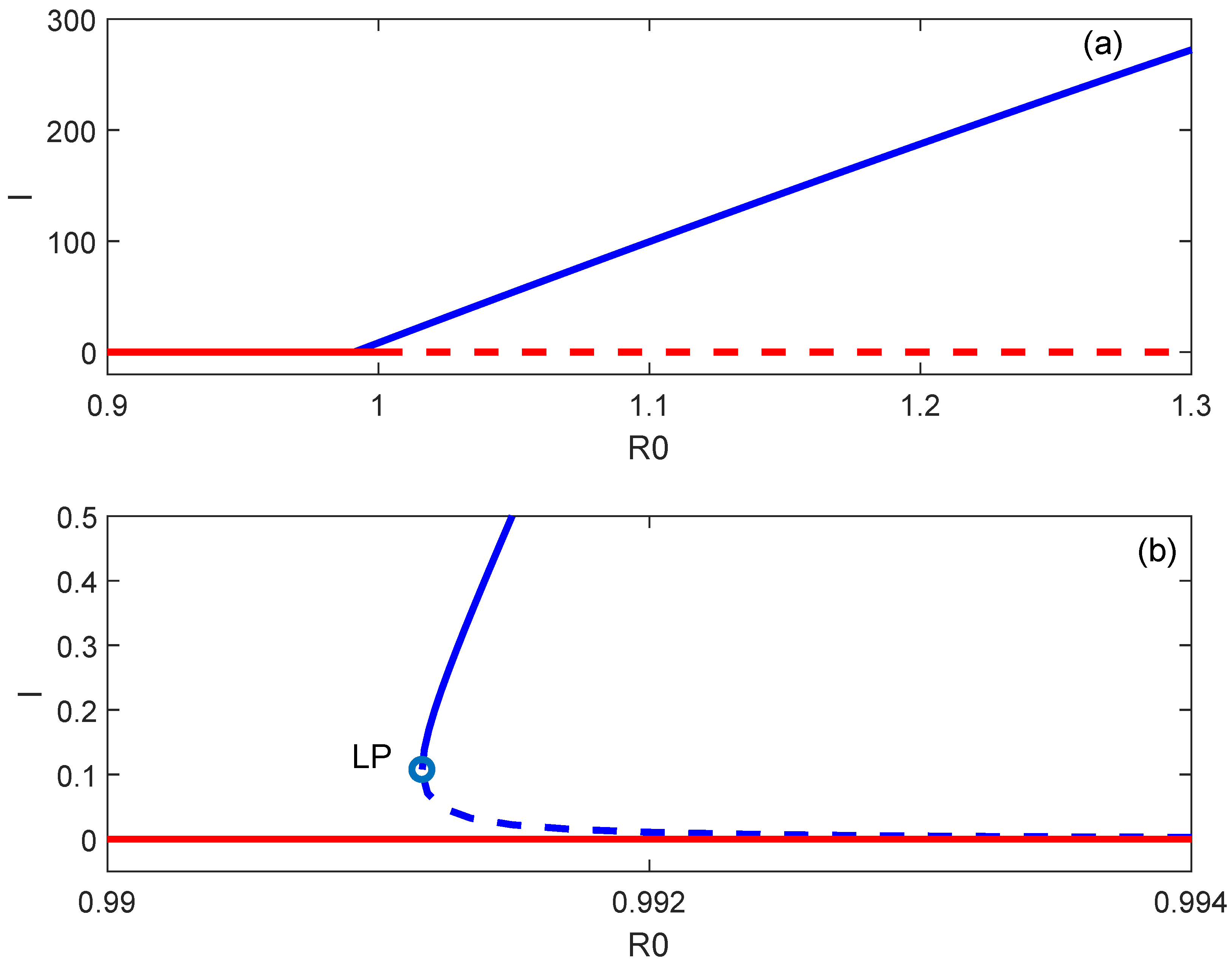
Figure 2 shows the bifurcation diagram for the case of fitted value  λ = 721.62 . This value is larger than the aforementioned critical value. A limit point (LP) was observed to occur at  R 0 = 0.9911 . Therefore, the disease-free equilibrium coexists with the stable endemic solution for any value of  R 0  between 0.9911 and 1. This diagram illustrates the important role health services (i.e.,  λ ) play in disease dynamics. To suppress the disease, it is insufficient to reduce  R 0  below unity; rather, it must be reduced to less than the limit point.
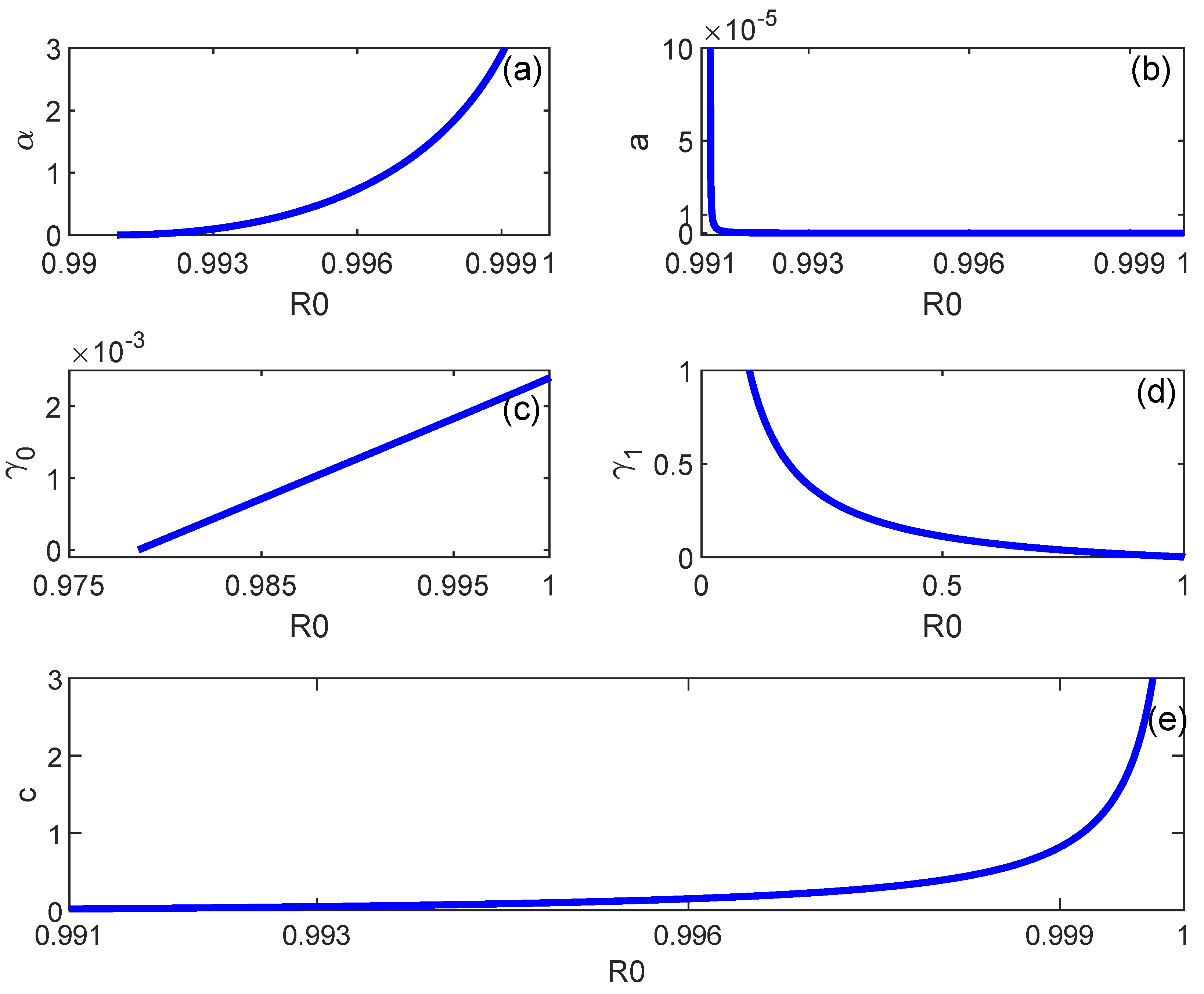
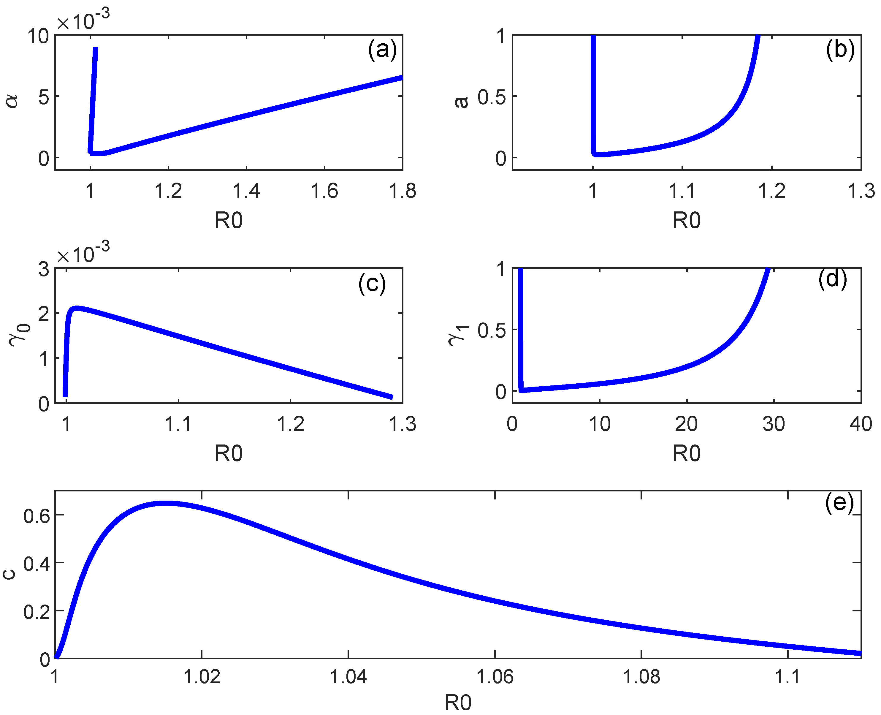
Next, we present the results of a sensitivity analysis for the effect of model parameters on the range of the backward bifurcation. Figure 3a–e show the locus of the limit point in the different parameter spaces. The effect of fear is shown in Figure 3a. As the fear parameter ( α ) increases, the limit point occurs at a larger reproduction number. Therefore, the range of coexistence of the stable disease-free equilibrium with the endemic solution decreases in terms of  R 0 . The increase in fear has an important effect in reducing backward bifurcation.
Figure 3b shows the effect of the inverse (a) of the latent period. It can be seen that the backward bifurcation increases if (a) increases. The effects of the minimum recovery rate ( γ 0 ) and maximum recovery rate ( γ 1 ) are shown in Figure 3c,d. It can be seen that the backward bifurcation is attenuated if the minimum recovery rate ( γ 0 ) increases and/or if the maximum recovery rate ( γ 1 ) decreases. Their roles appear to be important in reducing the backward bifurcation. Finally, Figure 3e shows that, as the coefficient of the treatment function increases, the limit point occurs at larger values of  R 0 , which means that the backward bifurcation is attenuated, as expected.
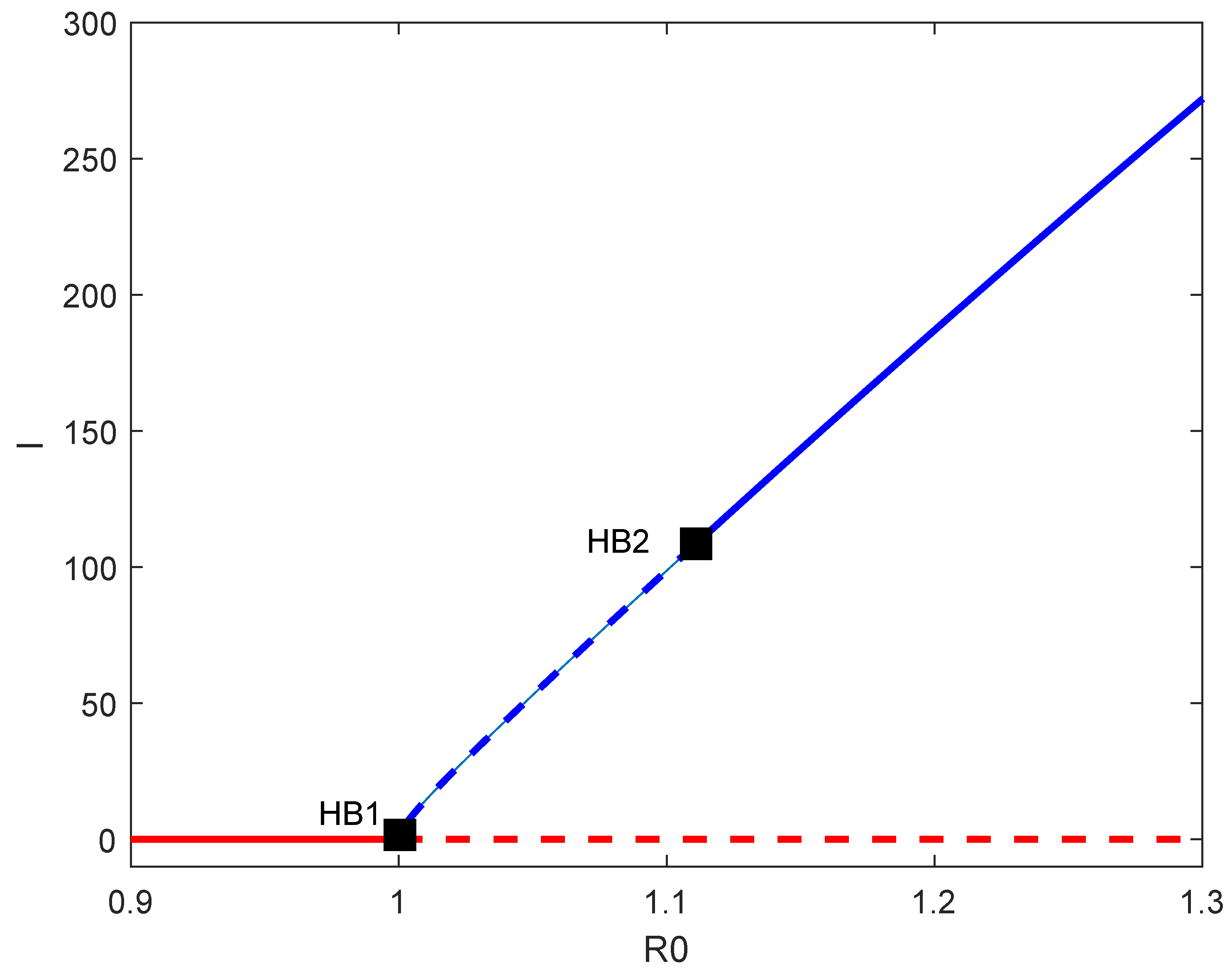
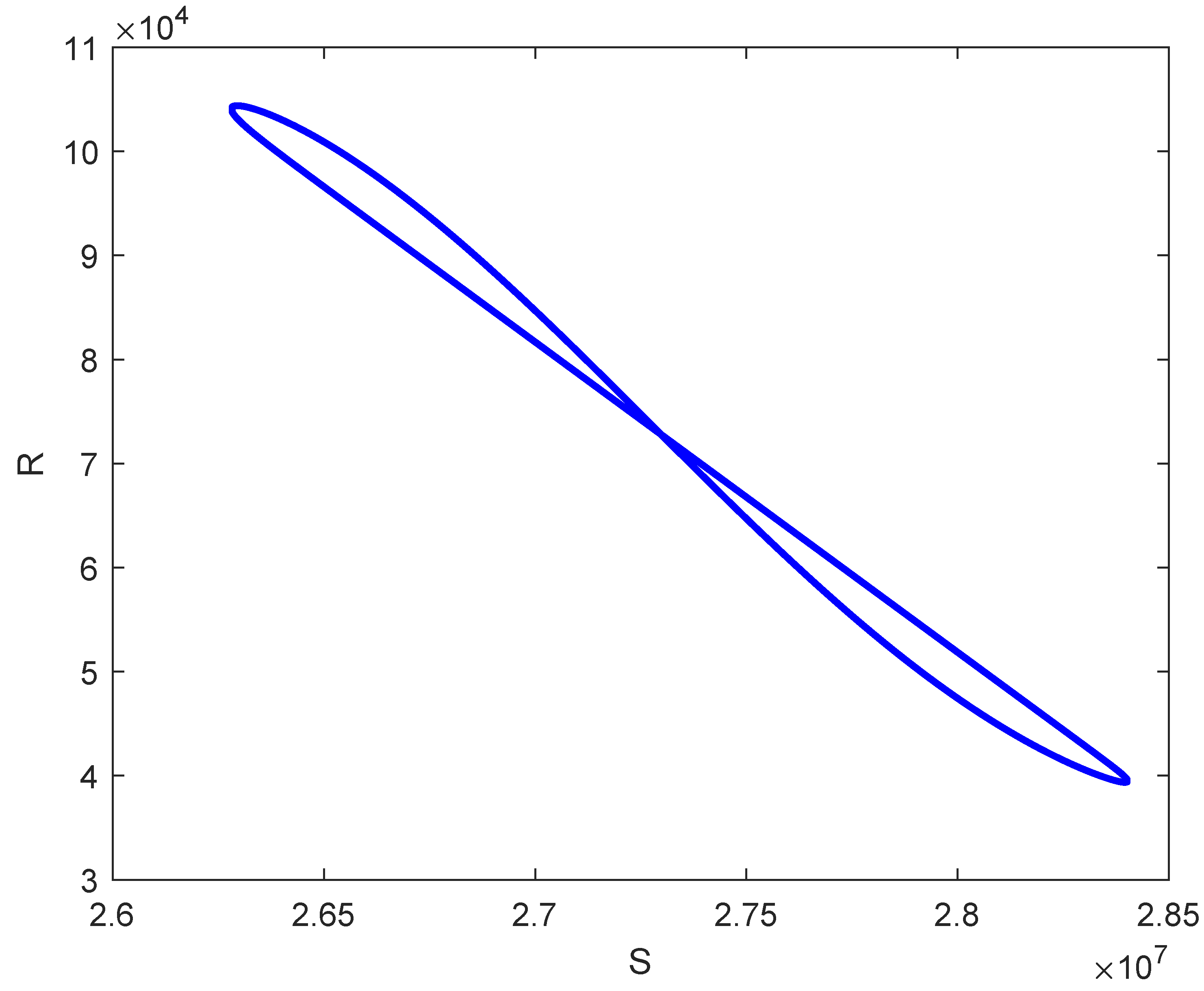
Conversely, Figure 4 shows the continuity diagram if  λ  is decreased to 0.111, just below the critical value of 0.12. The backward bifurcation is replaced by a forward bifurcation, in which the disease-free equilibrium is the only stable outcome for  R 0 < 1 . The disease is suppressed if the reproduction number is reduced below unity. However, the figure also predicts the existence of two Hopf points, which occur at  R 0 = 1.0004  and  R 0 = 1.111 . A stable periodic branch is expected between the two Hopf points, and Figure 5 shows an example of the limit cycle for  R 0 = 1.08 . Beyond the value of the second Hopf point, the model predicts a stable static branch. The existence of a stable periodic branch when the reproduction  R 0 > 1  is an interesting result because it shows that the disease incidents can fluctuate within a range of reproduction numbers, making the control and mitigation of the disease a very challenging task.
Next, we analyse the effect of model parameters on the occurrence of such oscillatory behaviour. Two-parameter continuation diagrams (Figure 6) are shown; the loci of the two Hopf points are depicted in each branch of each figure. Figure 6a shows the effect of fear. Hopf points exist only when the level of fear  α  is above a critical value (the minimum) at  α = 3.5 . Hopf points cannot exist without fear ( α = 0 ). As  α  increases, the range of the Hopf points increases in terms of the reproduction number.
The effect of the incubation period is shown in Figure 6b. Again, Hopf points exist only for a value of (a) larger than a critical value, and the periodic regime increases as the value of (a) increases. By contrast, Figure 6c shows that the periodic regime exists only if the minimum recovery rate  γ 0  falls below a critical value, whereas the opposite trend is observed for the maximum recovery rate (Figure 6d).
Finally, the effect of the coefficient of the treatment function (Figure 6e) shows that Hopf points exist only when the value of (c) is below a critical value. The range of periodic regime increases as (c) decreases.

8. Discussion

From a practical point of view, our analysis (Figure 2 and Figure 3) shows that backward bifurcation is the most likely scenario of the disease dynamics in the country. To suppress the disease, the basic reproduction number should be reduced not only below unity but also below the value corresponding to the limit point. However, except for the maximum recovery rate (Figure 3d), the range of the limit points in all the other figures is very small (from 0.99 to 0.999) and is not far from unity, even if the parameters vary widely. Therefore, practically, the backward bifurcation range is not significant.
The existence of periodic behaviour in the model is interesting but not unusual. Several studies have shown that the dynamics of the COVID-19 pandemic are complex. For example, Sapkota et al. [39] analysed time series of COVID-19 data and found evidence that the worldwide spread of COVID-19 showed complex and even chaotic behaviour. Other authors [40,41] have used simple models to predict periodic and non-periodic complex behaviour in the spread of COVID-19. The model proposed in this paper exhibited only simple periodic behaviour, but even this behaviour adds to the difficulty of controlling and preventing the pandemic. The diagrams in Figure 6 are useful to illustrate the effects of model parameters on the attenuation of this unwanted oscillatory behaviour.
Comparing the results predicted by our model with those of a previous work [19] that explored the effect of the number of hospital beds on the recovery rate, it can be noted that the results in [19] showed that the variable recovery rate led to more complex dynamics, such as a cusp-type Bogdanov–Takens bifurcation. Our model did not predict this latter behaviour, although it managed to predict the rest of the behaviours such as backward bifurcation and Hopf bifurcation. However, the model parameters used in the work carried out in [19] were general and not extracted from a validation study.
Regarding work on the impact of fear [28], our model managed to also predict the existence of a backward bifurcation for some levels of fear, meaning that the critical value of the reproduction number at the limit point can be used as a new threshold for disease control.

9. Conclusions

We proposed and analysed the dynamics of an SEIR model for COVID-19 transmission with three notable modifications: (1) the model accounts for the fear factor, (2) the recovery rate is nonlinear and depends on the quality of health services, and (3) the model considers a treatment function. Most of the model parameters were obtained by fitting the model to COVID-19 data from Saudi Arabia, providing the model with some credibility.
Two interesting behaviours were encountered in our analysis: (1) the static coexistence of the endemic equilibrium with the disease-free solution for values of the reproduction number between the limit point and unity and (2) the existence of stable oscillations for some range of reproduction numbers larger than one in the case of forward bifurcation.
We showed that the range of backward bifurcation is very small in terms of the values of the reproduction number. The range can be reduced with an increase in the quality of health services, an increase in the treatment, and an increase in the fear effect. The latter could be accomplished by increasing education and awareness through media. We also found that the periodic behaviour identified for the case of forward bifurcation is favoured by an increase in the quality of health services, an increase in the fear factor, and an increase in the treatment function.
Although simple in structure and old in conception, SEIR models can predict many dynamic behaviours that are exhibited by more complex models’ structures. We suggest three areas of future research to overcome the limitations of the current study. The model would be improved if its parameters were assumed to vary with time. These include parameters such as the incubation period and level of fear. The latter cannot realistically be constant since its value changes with the severity of the disease and the number of deaths. Another area of research is the refinement of the optimisation problem used for model validation with the goal of obtaining global solutions. The third area is to include the effect of vaccination on disease transmission. Mandatory vaccination was implemented in the country, but detailed data for daily vaccination are unfortunately not available.

Author Contributions

Methodology, R.T.A. and N.H.A.; Formal analysis, R.T.A. and A.A.; Investigation, A.A.; Resources, N.H.A.; Writing—original draft, A.A.; Writing—review editing, A.A. and N.H.A. All authors have read and agreed to the published version of the manuscript.

Funding

This research received no external funding.

Data Availability Statement

Data are contained within the article.

Conflicts of Interest

The authors declare no conflicts of interest.

Appendix A

Appendix A.1. Proof of Theorem 1

The proof is based on similar work in [42].
Let
m ( t ) = m i n ( S ( t ) , E ( t ) , I ( t ) , R ( t ) ) , t > 0
Clearly, we have  m ( 0 ) > 0 .  We assume that there exists a  t 1 > 0  such that  m ( t 1 ) = 0  and  m ( t ) > 0 , ∀ 0 t < t 1 . Let us start by showing that  S ( t ) > 0 . We assume that  m ( t 1 ) = S ( t 1 ) = 0 . Since  I ( t 1 ) > 0 0 t < t , and using Equation (1), we have that
d S d t S ( μ + β I ) .
Therefore,
S ( t 1 ) S 0 e x p ( 0 t 1 ( μ + β I ( s ) ) ) d s > 0 ,
which contradicts the assumption of  S ( t 1 ) = 0 .
Similarly, for  ( E ) , we assume that  m ( t 1 ) = E ( t 1 ) = 0 , then, from Equation (2), we have
d E d t ( μ + a ) E ,
which yields
E ( t 1 ) E 0 e x p ( 0 t 1 ( μ + a ) ) d s > 0 .
This contradicts the assumption  E ( t 1 ) = 0 .
Similarly, for  ( I ) , we assume  m ( t 1 ) = I ( t 1 ) = 0 , then, Equation (3) yields
d I d t ( μ + μ 1 + γ + c ) I ,
which yields
I ( t 1 ) I 0 e x p ( 0 t 1 ( μ + μ 1 + γ ( s ) + c ) I ( s ) ) d s > 0 .
This contradicts  I ( t 1 ) = 0 .
Finally, we assume  m ( t 1 ) = R ( t 1 ) = 0 , then, from Equation (4), we have
d R d t μ R ,
which yields
R ( t 1 ) R 0 e x p ( 0 t 1 μ R ( s ) ) d s > 0 ,
which contradicts the assumption  R ( t 1 ) = 0 .

Appendix A.2. Proof of Theorem 2

Let us denote  N ( t ) = S ( t ) + E ( t ) + I ( t ) + R ( t ) . We then have, from Equations (1)–(4), that
d N ( t ) d t = μ N ( t ) μ 1 I + Λ 1 + α I .
Therefore,
d N ( t ) d t μ N ( t ) + Λ 1 + α I μ N ( t ) + Λ ,
since the fear has the effect of decreasing the recruitment rate, i.e.,  Λ 1 + α I < Λ . Integrating Equation (A2) yields
N ( t ) N ( 0 ) exp ( μ t ) + Λ μ ( 1 exp ( μ t ) ) ,
where  N ( 0 )  is the initial condition of  N ( t ) . Therefore,  0 < N ( t ) < Λ μ  as t goes to  +  and  d N ( t ) d t < 0  for  N > Λ μ . This shows that  Ψ  is positively invariant.

References

  1. Khairulbahri, M. The SEIR model incorporating asymptomatic cases, behavioral measures, and lockdowns: Lesson learned from the COVID-19 flow in Sweden. Biomed. Signal Process. Control 2022, 81, 104416. [Google Scholar] [CrossRef] [PubMed]
  2. Kiselev, I.N.; Akberdin, I.R.; Kolpakov, F.A. Delay-differential SEIR modeling for improved modelling of infection dynamics. Sci. Rep. 2023, 13, 13439. [Google Scholar] [CrossRef] [PubMed]
  3. Papageorgiou, V.E.; Vasiliadis, G.; Tsaklidis, G. Analyzing the asymptotic behavior of an extended SEIR model with vaccination for COVID-19. Mathematics 2024, 12, 55. [Google Scholar] [CrossRef]
  4. Khalilpourazari, S.; Doulabi, H.H. Robust modelling and prediction of the COVID-19 pandemic in Canada. Int. J. Prod. Res. 2023, 61, 8367–8383. [Google Scholar] [CrossRef]
  5. Prathumwan, D.; Trachoo, K.; Chaiya, I. Mathematical modeling for prediction dynamics of the coronavirus disease 2019 (COVID-19) pandemic, quarantine control measures. Symmetry 2020, 12, 1404. [Google Scholar] [CrossRef]
  6. Feng, L.X.; Jing, S.L.; Hu, S.K.; Wang, D.F.; Huo, H.F. Modelling the effects of media coverage and quarantine on the COVID-19 infections in the UK. Math. Biosci. Eng. 2020, 17, 3618–3636. [Google Scholar] [CrossRef]
  7. Sardar, T.; Nadim, S.; Rana, S.; Chattopadhyay, J. Assessment of lockdown effect in some states and overall India: A predictive mathematical study on COVID-19 outbreak. Chaos Solit. Fractals 2020, 139, 110078. [Google Scholar] [CrossRef]
  8. Francesco, P.; Lorenzo, Z.; Maurizio, P.; Alessandro, R. Modelling and predicting the effect of social distancing and travel restrictions on COVID-19 spreading. J. R. Soc. Interface 2021, 18, 182020087520200875. [Google Scholar]
  9. Rahimi, I.; Chen, F.; Gandomi, A.H. A review on COVID-19 forecasting models. Neural Comput. Appl. 2023, 35, 23671–23681. [Google Scholar] [CrossRef]
  10. Gnanvi, J.E.; Salako, K.V.; Kotanmi, G.B.; Kakai, R.G. On the reliability of predictions on COVID-19 dynamics: A systematic and critical review of modelling techniques. Infect. Dis. Model. 2021, 6, 258–272. [Google Scholar] [CrossRef]
  11. Roosa, K.; Lee, Y.; Luo, R.; Kirpich, A.; Rothenberg, R.; Hyman, J.M.; Yan, P.; Chowell, G. Short-term forecasts of the COVID-19 epidemic in Guangdong and Zhejiang. J. Clin. Med. 2020, 9, 596. [Google Scholar] [CrossRef]
  12. Ajbar, A.; Alqahtani, R.T. Bifurcation analysis of a SEIR epidemic system with governmental action and individual reaction. Adv. Differ. Equ. 2020, 2020, 541. [Google Scholar] [CrossRef] [PubMed]
  13. Das, R.C. Forecasting incidences of COVID-19 using Box-Jenkins method for the period 12 July –11 September 2020: A study on highly affected countries. Chaos Solit. Fractals 2020, 2020, 140. [Google Scholar]
  14. Sher, M.; Shah, K.; Khan, Z.A.; Khan, H.; Khan, A. Computational and theoretical modeling of the transmission dynamics of novel COVID-19 under Mittag–Leffler Power law. Alex. Eng. J. 2020, 59, 3133–3147. [Google Scholar] [CrossRef]
  15. Dokuyucu, M.A.; Celik, E. Analyzing a novel coronavirus model (COVID-19) in the sense of Caputo-Fabrizio fractional operator. Appl. Comput. Math. Ean. Int. J. 2021, 20, 49–69. [Google Scholar]
  16. Namasudra, S.; Dhamodharavadhani, S.; Rathipriya, R. Nonlinear neural network based forecasting model for predicting COVID-19 Cases. Neural Process Lett. 2023, 55, 171–191. [Google Scholar] [CrossRef] [PubMed]
  17. Xiang, Y.; Jia, Y.; Chen, L.; Guo, L.; Shu, B.; Long, E. COVID-19 epidemic prediction and the impact of public health interventions: A review of COVID-19 epidemic models. Infect. Dis. Model. 2021, 6, 324–342. [Google Scholar] [CrossRef]
  18. Hu, Z.; Ma, W.; Ruan, S. Analysis of SIR epidemic models with nonlinear incidence rate and treatment. Math. Biosci. 2012, 238, 12–20. [Google Scholar] [CrossRef]
  19. Chan, C.; Zhu, H. Bifurcations and complex dynamics of an SIR model with the impact of the number of hospital beds. J. Diff. Equ. 2014, 257, 1662–1688. [Google Scholar]
  20. Cui, Q.; Qiu, Z.; Liu, W.; Hu, Z. Complex dynamics of an SIR epidemic model with nonlinear saturate incidence and recovery rate. Entropy 2017, 19, 305. [Google Scholar] [CrossRef]
  21. Epstein, J.M.; Parker, J.; Cummings, D.; Hammond, R.A. Coupled contagion dynamics of fear and disease: Mathematical and computational explorations. PLoS ONE 2008, 3, e3955. [Google Scholar] [CrossRef] [PubMed]
  22. Valle, S.; Mniszewski, S.; Hyman, J. Modeling the impact of behavior changes on the spread of pandemic influenza. In Modeling the Interplay between Human Behavior and the Spread of Infectious Diseases; Manfredi, P., d’Onofrio, A., Eds.; Springer Science & Business Media: New York, NY, USA, 2012; pp. 59–77. [Google Scholar]
  23. Bozkurt, F.; Yousef, A.; Abdeljawad, T.; Kalinli, A.; Al-Mdallal, Q. A fractional-order model of COVID-19 considering the fear effect of the media and social networks on the community. Chaos Solit. Fractals 2021, 152, 111403. [Google Scholar] [CrossRef]
  24. Rajabi, A.; Mantzaris, A.V.; Mutlu, E.C.; Garibay, O.O. Investigating dynamics of COVID-19 spread and containment with agent-based modeling. Appl. Sci. 2021, 11, 5367. [Google Scholar] [CrossRef]
  25. Maji, C. Impact of media-induced fear on the control of COVID-19 outbreak: A mathematical study. Int. J. Differ. Equ. 2021, 2021, 2129490. [Google Scholar] [CrossRef]
  26. Mpeshe, S.C.; Nyerere, N. Modeling the dynamics of coronavirus disease pandemic coupled with fear epidemics. Comput. Math. Methods Med. 2021, 2021, 6647425. [Google Scholar] [CrossRef] [PubMed]
  27. Zhou, L.L.; Ampon-Wireko, S.; Xu, X.L.; Quansah, P.E.; Larnyo, E. Media attention and vaccine hesitancy: Examining the mediating effects of fear of COVID-19 and the moderating role of trust in leadership. PLoS ONE 2022, 17, e0263610. [Google Scholar] [CrossRef] [PubMed]
  28. Thirthar, A.A.; Abboubakar, H.; Khan, A.; Abdeljawad, T. Mathematical modeling of the COVID-19 epidemic with fear impact. J. AIMS Math. 2023, 8, 6447–6465. [Google Scholar] [CrossRef]
  29. Wang, W.; Ruan, S. Bifurcations in an epidemic model with constant removal rate of incentives. J. Math. Anal. Appl. 2004, 291, 775–793. [Google Scholar] [CrossRef]
  30. Wang, W. Backward Bifurcation of an Epidemic Model with Treatment. Math. Biosci. 2006, 201, 58–71. [Google Scholar] [CrossRef]
  31. Zhang, X.; Liu, X. Backward bifurcation of an epidemic model with saturated treatment. J. Math. Anal. Appl. 2008, 348, 433–443. [Google Scholar] [CrossRef]
  32. Van den Driessche, P.; Watmough, J. Reproduction numbers and subthreshold endemic equilibria for compartmental models of disease transmission. Math. Biosci. 2002, 180, 29–48. [Google Scholar] [CrossRef] [PubMed]
  33. Castillo-Chavez, C.; Song, B. Dynamical models of tuberculosis and their applications. Math. Biosci. Eng. 2004, 1, 361–404. [Google Scholar] [CrossRef] [PubMed]
  34. Available online: https://www.worldometers.info/coronavirus/country/saudi-arabia/ (accessed on 6 March 2024).
  35. General Authority for Statistics, Saudi Arabia. Available online: https://www.stats.gov.sa/en/5305 (accessed on 6 March 2024).
  36. MATLAB Version: 9.4 (R2018a); The MathWorks Inc.: Natick, MA, USA, 2018.
  37. Aletreby, W.T.; Alharthy, A.M.; Faqihi, F.; Mady, A.F.; Ramadan, O.E.; Huwait, B.M.; Alodat, M.A.; Lahmar, A.B.; Mahmood, N.N.; Mumtaz, S.A.; et al. Dynamics of SARS-CoV-2 outbreak in the Kingdom of Saudi Arabia: A predictive model. Saudi Crit. Care. J. 2020, 4, 79–83. [Google Scholar] [CrossRef]
  38. Alshammari, F. A Mathematical model to investigate the transmission of COVID-19 in the kingdom of Saudi Arabia. Comput. Math. Method Med. 2020, 2020, 9136157. [Google Scholar] [CrossRef]
  39. Sapkota, N.; Karwowski, W.; Davahli, M.R.; Al-Juaid, A.; Taiar, R.; Murata, A. The chaotic behavior of the spread of infection during the COVID-19 pandemic in the United States and globally. IEEE Access 2021, 9, 0692–80702. [Google Scholar] [CrossRef] [PubMed]
  40. Brugnago, E.L.; Gabrick, E.C.; Iarosz, K.C.; Szezech, J.D.; Viana, R.L.; Batista, A.M.; Caldas, I.L. Multistability and chaos in SEIRS epidemic model with a periodic time-dependent transmission rate. Chaos 2023, 33, 123123. [Google Scholar] [CrossRef] [PubMed]
  41. Buonomo, B.; Giacobbe, A. Oscillations in SIR behavioural epidemic models: The interplay between behaviour and overexposure to infection. Chaos Solit. Fractals 2023, 174, 113782. [Google Scholar] [CrossRef]
  42. Li, Y.; Teng, Z.; Ruan, S.; Li, M.; Feng, X. A mathematical model for the seasonal transmission of schistosomiasis in the lake and marshland regions of China. Math. Biosci. Eng. 2017, 14, 1279–1299. [Google Scholar] [CrossRef]
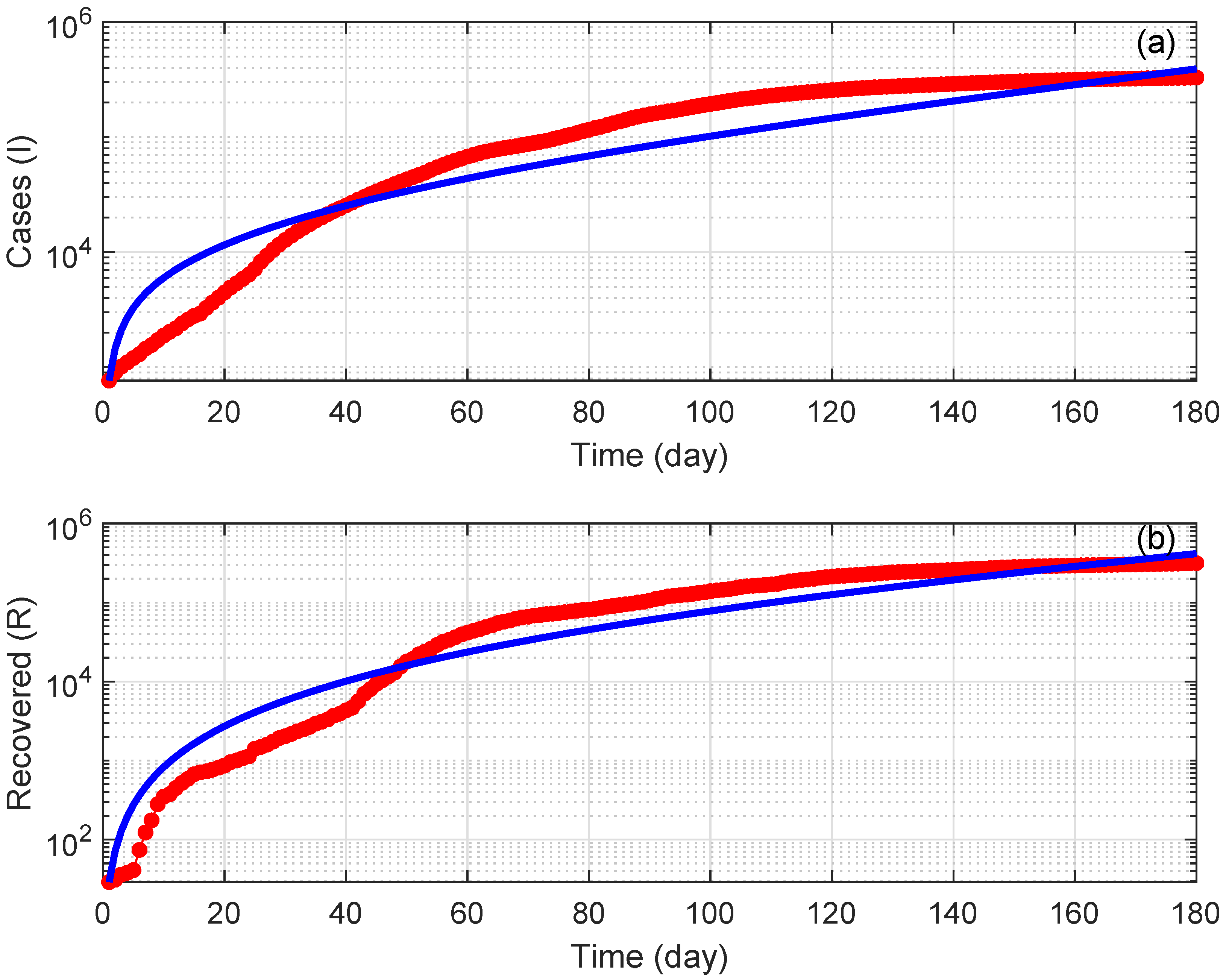
Figure 1. Results of fitting the model to COVID-19 cases in Saudi Arabia for a period of 6 months starting from 2 March 2020. Red color, COVID-19 data; blue color, model. (a): infectious cases (I); (b): the combined recovered and deceased cases (R).
Mathematics 12 01678 g001
Figure 2. (a) Bifurcation diagram for  λ = 721.62  showing backward bifurcation; (b) enlargement of (a) around  R 0 = 1 . Solid line (stable branch); dashed line (unstable branch); LP (static limit point).
Mathematics 12 01678 g002
Figure 3. Two-parameter continuation diagrams showing the locus of the limit point of Figure 2b; (a) Effect of fear level ( α ); (b) Effect of inverse of incubation period (a); (c) Effect of minimum value of recovery rate ( γ 0 ); (d) Effect of maximum value of recovery rate ( γ 1 ); (e) Effect of coefficient of treatment (c).
Mathematics 12 01678 g003
Figure 4. Bifurcation diagram for  λ = 0.11  showing forward bifurcation; solid line (stable branch); dashed line (unstable branch); HB, Hopf point.
Mathematics 12 01678 g004
Figure 5. Limit cycle for  R 0 = 1.08  of Figure 4.
Mathematics 12 01678 g005
Figure 6. Two-parameter continuation diagrams showing the loci of Hopf points of Figure 4; (a) Effect of fear level ( α ); (b) Effect of inverse of incubation period (a); (c) Effect of minimum value of recovery rate ( γ 0 ); (d) Effect of maximum value of recovery rate ( γ 1 ); (e) Effect of coefficient of treatment (c).
Mathematics 12 01678 g006
Table 1. Number of positive roots of Equations (17) and (18).
Case a 3 a 2 a 1 a 0 R 0 Number of Sign ChangesNumber of Positive Roots
1--++ > 1 11
2---+ > 1 11
3--+- < 1 20.2
4---- < 1 00
Table 2. Model parameters.
ParameterDefinitionValueSource
aInverse of mean latent period 0.155 fitted
cTreatment function factor 1.78 × 10 2 fitted
α Fear effect factor 10 3 fitted
λ Quality of health services factor 721.62 fitted
γ 0 Minimum recovery rate 1.4 × 10 3 fitted
γ 1 Maximum recovery rate2 . 4 × 10 3 fitted
μ Natural death rate 4.21 × 10 5 [35]
μ 1 Mortality due to the disease 0.09 [35]
Λ Recruitment rate1252[35]
Disclaimer/Publisher’s Note: The statements, opinions and data contained in all publications are solely those of the individual author(s) and contributor(s) and not of MDPI and/or the editor(s). MDPI and/or the editor(s) disclaim responsibility for any injury to people or property resulting from any ideas, methods, instructions or products referred to in the content.