
Dynamics of a Model of Coronavirus Disease with Fear Effect, Treatment Function, and Variable Recovery Rate


Abstract
1. Introduction
2. The Transmission Model
3. Basic Properties
4. Disease-Free Equilibrium and Reproduction Number
4.1. Disease-Free Equilibrium
4.2. Basic Reproduction Number
4.3. Local Stability of the Disease-Free Equilibrium
5. Endemic Equilibria
- 1.
- Possesses one steady state if ;
- 2.
- Can possess up to two steady states if .
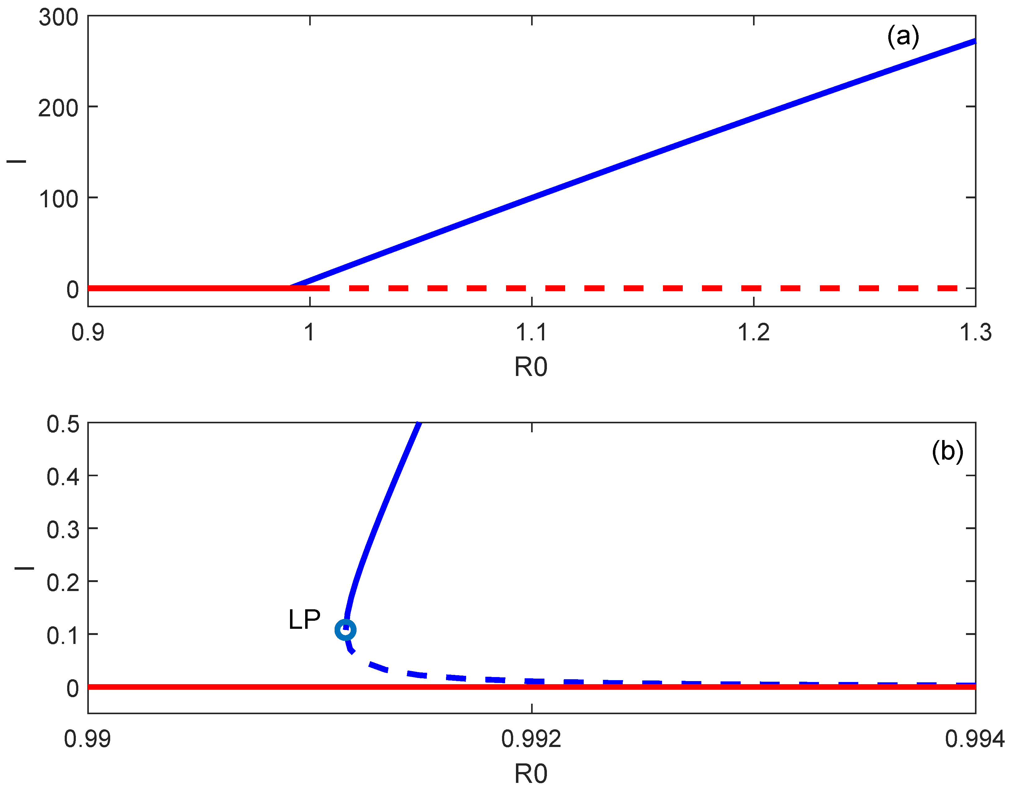
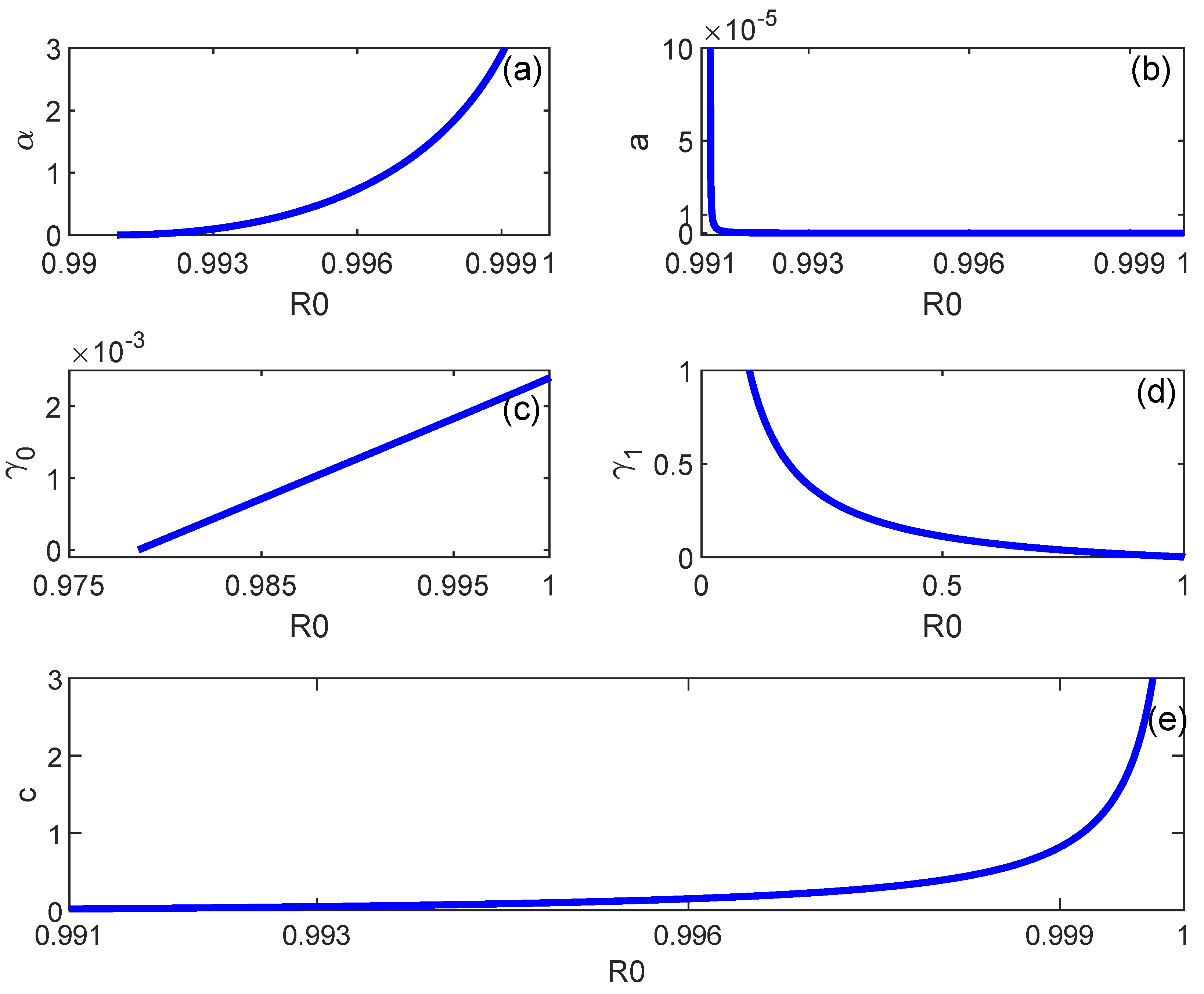
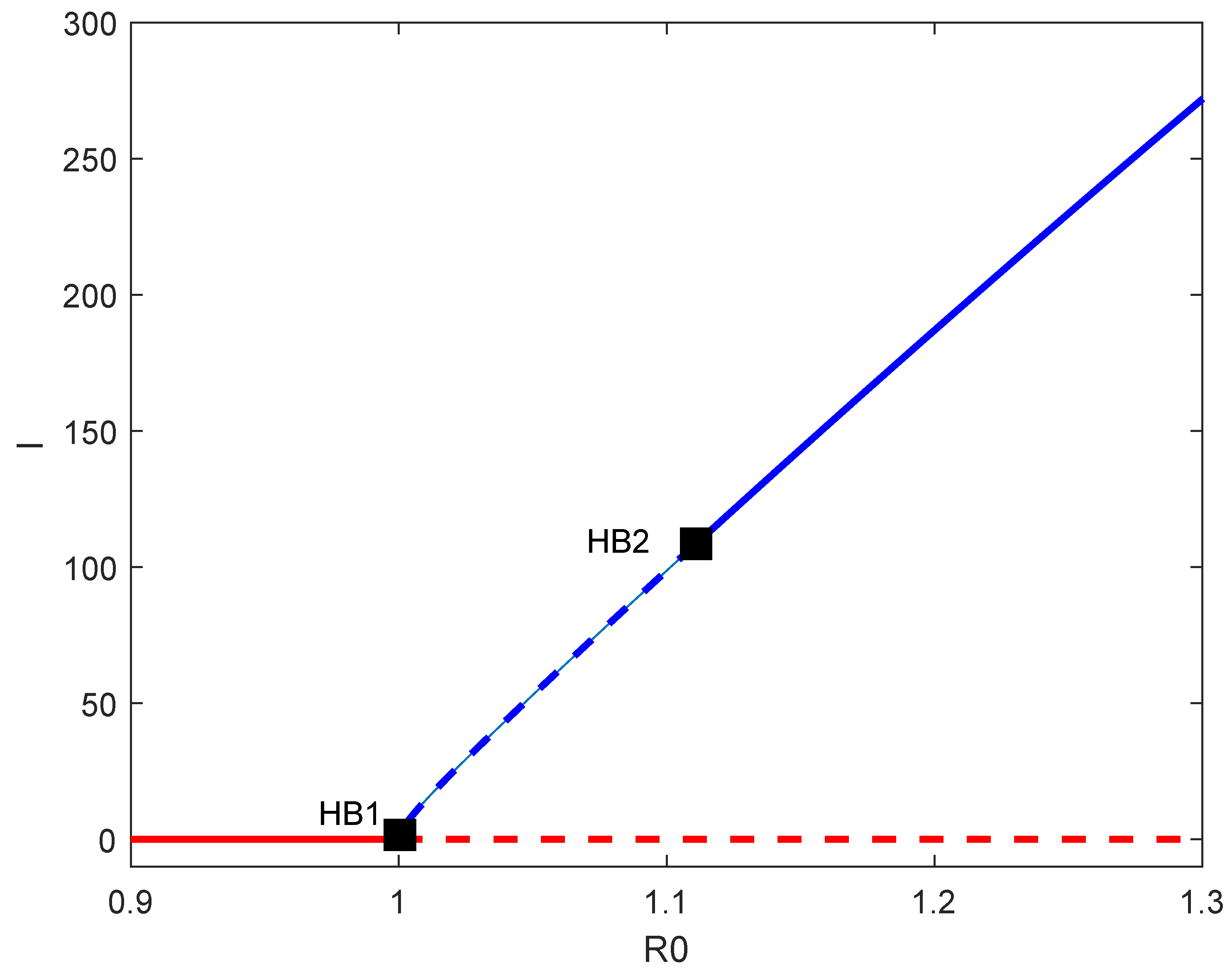
6. Backward Bifurcation
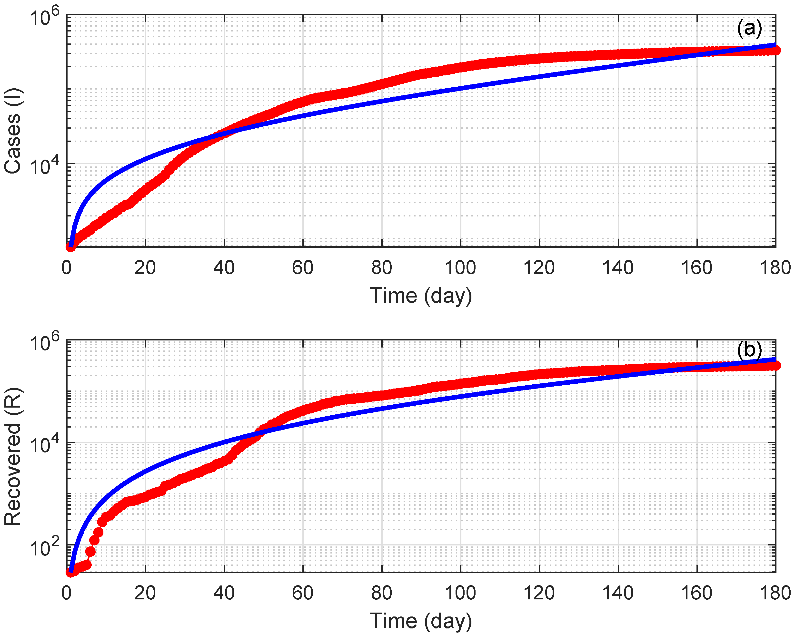
7. Numerical Simulations
8. Discussion
9. Conclusions
Author Contributions
Funding
Data Availability Statement
Conflicts of Interest
Appendix A
Appendix A.1. Proof of Theorem 1
Appendix A.2. Proof of Theorem 2
References
- Khairulbahri, M. The SEIR model incorporating asymptomatic cases, behavioral measures, and lockdowns: Lesson learned from the COVID-19 flow in Sweden. Biomed. Signal Process. Control 2022, 81, 104416. [Google Scholar] [CrossRef] [PubMed]
- Kiselev, I.N.; Akberdin, I.R.; Kolpakov, F.A. Delay-differential SEIR modeling for improved modelling of infection dynamics. Sci. Rep. 2023, 13, 13439. [Google Scholar] [CrossRef] [PubMed]
- Papageorgiou, V.E.; Vasiliadis, G.; Tsaklidis, G. Analyzing the asymptotic behavior of an extended SEIR model with vaccination for COVID-19. Mathematics 2024, 12, 55. [Google Scholar] [CrossRef]
- Khalilpourazari, S.; Doulabi, H.H. Robust modelling and prediction of the COVID-19 pandemic in Canada. Int. J. Prod. Res. 2023, 61, 8367–8383. [Google Scholar] [CrossRef]
- Prathumwan, D.; Trachoo, K.; Chaiya, I. Mathematical modeling for prediction dynamics of the coronavirus disease 2019 (COVID-19) pandemic, quarantine control measures. Symmetry 2020, 12, 1404. [Google Scholar] [CrossRef]
- Feng, L.X.; Jing, S.L.; Hu, S.K.; Wang, D.F.; Huo, H.F. Modelling the effects of media coverage and quarantine on the COVID-19 infections in the UK. Math. Biosci. Eng. 2020, 17, 3618–3636. [Google Scholar] [CrossRef]
- Sardar, T.; Nadim, S.; Rana, S.; Chattopadhyay, J. Assessment of lockdown effect in some states and overall India: A predictive mathematical study on COVID-19 outbreak. Chaos Solit. Fractals 2020, 139, 110078. [Google Scholar] [CrossRef]
- Francesco, P.; Lorenzo, Z.; Maurizio, P.; Alessandro, R. Modelling and predicting the effect of social distancing and travel restrictions on COVID-19 spreading. J. R. Soc. Interface 2021, 18, 182020087520200875. [Google Scholar]
- Rahimi, I.; Chen, F.; Gandomi, A.H. A review on COVID-19 forecasting models. Neural Comput. Appl. 2023, 35, 23671–23681. [Google Scholar] [CrossRef]
- Gnanvi, J.E.; Salako, K.V.; Kotanmi, G.B.; Kakai, R.G. On the reliability of predictions on COVID-19 dynamics: A systematic and critical review of modelling techniques. Infect. Dis. Model. 2021, 6, 258–272. [Google Scholar] [CrossRef]
- Roosa, K.; Lee, Y.; Luo, R.; Kirpich, A.; Rothenberg, R.; Hyman, J.M.; Yan, P.; Chowell, G. Short-term forecasts of the COVID-19 epidemic in Guangdong and Zhejiang. J. Clin. Med. 2020, 9, 596. [Google Scholar] [CrossRef]
- Ajbar, A.; Alqahtani, R.T. Bifurcation analysis of a SEIR epidemic system with governmental action and individual reaction. Adv. Differ. Equ. 2020, 2020, 541. [Google Scholar] [CrossRef] [PubMed]
- Das, R.C. Forecasting incidences of COVID-19 using Box-Jenkins method for the period 12 July –11 September 2020: A study on highly affected countries. Chaos Solit. Fractals 2020, 2020, 140. [Google Scholar]
- Sher, M.; Shah, K.; Khan, Z.A.; Khan, H.; Khan, A. Computational and theoretical modeling of the transmission dynamics of novel COVID-19 under Mittag–Leffler Power law. Alex. Eng. J. 2020, 59, 3133–3147. [Google Scholar] [CrossRef]
- Dokuyucu, M.A.; Celik, E. Analyzing a novel coronavirus model (COVID-19) in the sense of Caputo-Fabrizio fractional operator. Appl. Comput. Math. Ean. Int. J. 2021, 20, 49–69. [Google Scholar]
- Namasudra, S.; Dhamodharavadhani, S.; Rathipriya, R. Nonlinear neural network based forecasting model for predicting COVID-19 Cases. Neural Process Lett. 2023, 55, 171–191. [Google Scholar] [CrossRef] [PubMed]
- Xiang, Y.; Jia, Y.; Chen, L.; Guo, L.; Shu, B.; Long, E. COVID-19 epidemic prediction and the impact of public health interventions: A review of COVID-19 epidemic models. Infect. Dis. Model. 2021, 6, 324–342. [Google Scholar] [CrossRef]
- Hu, Z.; Ma, W.; Ruan, S. Analysis of SIR epidemic models with nonlinear incidence rate and treatment. Math. Biosci. 2012, 238, 12–20. [Google Scholar] [CrossRef]
- Chan, C.; Zhu, H. Bifurcations and complex dynamics of an SIR model with the impact of the number of hospital beds. J. Diff. Equ. 2014, 257, 1662–1688. [Google Scholar]
- Cui, Q.; Qiu, Z.; Liu, W.; Hu, Z. Complex dynamics of an SIR epidemic model with nonlinear saturate incidence and recovery rate. Entropy 2017, 19, 305. [Google Scholar] [CrossRef]
- Epstein, J.M.; Parker, J.; Cummings, D.; Hammond, R.A. Coupled contagion dynamics of fear and disease: Mathematical and computational explorations. PLoS ONE 2008, 3, e3955. [Google Scholar] [CrossRef] [PubMed]
- Valle, S.; Mniszewski, S.; Hyman, J. Modeling the impact of behavior changes on the spread of pandemic influenza. In Modeling the Interplay between Human Behavior and the Spread of Infectious Diseases; Manfredi, P., d’Onofrio, A., Eds.; Springer Science & Business Media: New York, NY, USA, 2012; pp. 59–77. [Google Scholar]
- Bozkurt, F.; Yousef, A.; Abdeljawad, T.; Kalinli, A.; Al-Mdallal, Q. A fractional-order model of COVID-19 considering the fear effect of the media and social networks on the community. Chaos Solit. Fractals 2021, 152, 111403. [Google Scholar] [CrossRef]
- Rajabi, A.; Mantzaris, A.V.; Mutlu, E.C.; Garibay, O.O. Investigating dynamics of COVID-19 spread and containment with agent-based modeling. Appl. Sci. 2021, 11, 5367. [Google Scholar] [CrossRef]
- Maji, C. Impact of media-induced fear on the control of COVID-19 outbreak: A mathematical study. Int. J. Differ. Equ. 2021, 2021, 2129490. [Google Scholar] [CrossRef]
- Mpeshe, S.C.; Nyerere, N. Modeling the dynamics of coronavirus disease pandemic coupled with fear epidemics. Comput. Math. Methods Med. 2021, 2021, 6647425. [Google Scholar] [CrossRef] [PubMed]
- Zhou, L.L.; Ampon-Wireko, S.; Xu, X.L.; Quansah, P.E.; Larnyo, E. Media attention and vaccine hesitancy: Examining the mediating effects of fear of COVID-19 and the moderating role of trust in leadership. PLoS ONE 2022, 17, e0263610. [Google Scholar] [CrossRef] [PubMed]
- Thirthar, A.A.; Abboubakar, H.; Khan, A.; Abdeljawad, T. Mathematical modeling of the COVID-19 epidemic with fear impact. J. AIMS Math. 2023, 8, 6447–6465. [Google Scholar] [CrossRef]
- Wang, W.; Ruan, S. Bifurcations in an epidemic model with constant removal rate of incentives. J. Math. Anal. Appl. 2004, 291, 775–793. [Google Scholar] [CrossRef]
- Wang, W. Backward Bifurcation of an Epidemic Model with Treatment. Math. Biosci. 2006, 201, 58–71. [Google Scholar] [CrossRef]
- Zhang, X.; Liu, X. Backward bifurcation of an epidemic model with saturated treatment. J. Math. Anal. Appl. 2008, 348, 433–443. [Google Scholar] [CrossRef]
- Van den Driessche, P.; Watmough, J. Reproduction numbers and subthreshold endemic equilibria for compartmental models of disease transmission. Math. Biosci. 2002, 180, 29–48. [Google Scholar] [CrossRef] [PubMed]
- Castillo-Chavez, C.; Song, B. Dynamical models of tuberculosis and their applications. Math. Biosci. Eng. 2004, 1, 361–404. [Google Scholar] [CrossRef] [PubMed]
- Available online: https://www.worldometers.info/coronavirus/country/saudi-arabia/ (accessed on 6 March 2024).
- General Authority for Statistics, Saudi Arabia. Available online: https://www.stats.gov.sa/en/5305 (accessed on 6 March 2024).
- MATLAB Version: 9.4 (R2018a); The MathWorks Inc.: Natick, MA, USA, 2018.
- Aletreby, W.T.; Alharthy, A.M.; Faqihi, F.; Mady, A.F.; Ramadan, O.E.; Huwait, B.M.; Alodat, M.A.; Lahmar, A.B.; Mahmood, N.N.; Mumtaz, S.A.; et al. Dynamics of SARS-CoV-2 outbreak in the Kingdom of Saudi Arabia: A predictive model. Saudi Crit. Care. J. 2020, 4, 79–83. [Google Scholar] [CrossRef]
- Alshammari, F. A Mathematical model to investigate the transmission of COVID-19 in the kingdom of Saudi Arabia. Comput. Math. Method Med. 2020, 2020, 9136157. [Google Scholar] [CrossRef]
- Sapkota, N.; Karwowski, W.; Davahli, M.R.; Al-Juaid, A.; Taiar, R.; Murata, A. The chaotic behavior of the spread of infection during the COVID-19 pandemic in the United States and globally. IEEE Access 2021, 9, 0692–80702. [Google Scholar] [CrossRef] [PubMed]
- Brugnago, E.L.; Gabrick, E.C.; Iarosz, K.C.; Szezech, J.D.; Viana, R.L.; Batista, A.M.; Caldas, I.L. Multistability and chaos in SEIRS epidemic model with a periodic time-dependent transmission rate. Chaos 2023, 33, 123123. [Google Scholar] [CrossRef] [PubMed]
- Buonomo, B.; Giacobbe, A. Oscillations in SIR behavioural epidemic models: The interplay between behaviour and overexposure to infection. Chaos Solit. Fractals 2023, 174, 113782. [Google Scholar] [CrossRef]
- Li, Y.; Teng, Z.; Ruan, S.; Li, M.; Feng, X. A mathematical model for the seasonal transmission of schistosomiasis in the lake and marshland regions of China. Math. Biosci. Eng. 2017, 14, 1279–1299. [Google Scholar] [CrossRef]

| Case | Number of Sign Changes | Number of Positive Roots | |||||
|---|---|---|---|---|---|---|---|
| 1 | - | - | + | + | 1 | 1 | 1 |
| 2 | - | - | - | + | 1 | 1 | 1 |
| 3 | - | - | + | - | 1 | 2 | 0.2 |
| 4 | - | - | - | - | 1 | 0 | 0 |
| Parameter | Definition | Value | Source |
|---|---|---|---|
| a | Inverse of mean latent period | fitted | |
| c | Treatment function factor | fitted | |
| Fear effect factor | fitted | ||
| Quality of health services factor | fitted | ||
| Minimum recovery rate | fitted | ||
| Maximum recovery rate | 2 | fitted | |
| Natural death rate | [35] | ||
| Mortality due to the disease | [35] | ||
| Recruitment rate | 1252 | [35] |
Disclaimer/Publisher’s Note: The statements, opinions and data contained in all publications are solely those of the individual author(s) and contributor(s) and not of MDPI and/or the editor(s). MDPI and/or the editor(s) disclaim responsibility for any injury to people or property resulting from any ideas, methods, instructions or products referred to in the content. |
© 2024 by the authors. Licensee MDPI, Basel, Switzerland. This article is an open access article distributed under the terms and conditions of the Creative Commons Attribution (CC BY) license (https://creativecommons.org/licenses/by/4.0/).
Share and Cite
Alqahtani, R.T.; Ajbar, A.; Alharthi, N.H. Dynamics of a Model of Coronavirus Disease with Fear Effect, Treatment Function, and Variable Recovery Rate. Mathematics 2024, 12, 1678. https://doi.org/10.3390/math12111678
Alqahtani RT, Ajbar A, Alharthi NH. Dynamics of a Model of Coronavirus Disease with Fear Effect, Treatment Function, and Variable Recovery Rate. Mathematics. 2024; 12(11):1678. https://doi.org/10.3390/math12111678
Chicago/Turabian StyleAlqahtani, Rubayyi T., Abdelhamid Ajbar, and Nadiyah Hussain Alharthi. 2024. "Dynamics of a Model of Coronavirus Disease with Fear Effect, Treatment Function, and Variable Recovery Rate" Mathematics 12, no. 11: 1678. https://doi.org/10.3390/math12111678
APA StyleAlqahtani, R. T., Ajbar, A., & Alharthi, N. H. (2024). Dynamics of a Model of Coronavirus Disease with Fear Effect, Treatment Function, and Variable Recovery Rate. Mathematics, 12(11), 1678. https://doi.org/10.3390/math12111678