Abstract
An acceptance sampling plan is a method used to make a decision about acceptance or rejection of a product based on adherence to a standard. Meanwhile, prior information, such as the process capability index (PCI), has been applied in different manufacturing industries to improve the quality of manufacturing processes and the quality inspection of products. In this paper, an attribute sampling plan is developed for submitted lots based on prior information and Bayesian approach. The new attribute sampling plans adjust sample sizes to prior information based on the status of the inspection target. To be specific, the sampling plans in this paper are indexed by the parameter trust with levels of low, medium, and high, where increasing trust level reduces sample size or risk. PCIs are an important basis for the choice of the trust level. In addition, multiple comparisons have been performed, including producer’s risk and consumer’s risk under different prior information parameters and different sample sizes.
Keywords:
beta distribution; Bayesian approach; producer’s risk; consumer’s risk; sample size; sampling plan MSC:
62G10; 62G20
1. Introduction
The primary objective of any production company is to enhance quality, and they typically adopt various strategies to achieve this goal. Among these strategies, inspection plays a pivotal role in upholding high standards. Acceptance sampling plans are frequently utilized as a quality control tool across various industrial contexts for conducting inspections (see [1,2,3] and so on)—in particular, in specific industrial sectors, such as the medical device and food industries, where the use of sampling policies is imposed by regulatory authorities. Schilling et al. [4] listed 10 reasons for the use of acceptance sampling in modern quality assurance. Acceptance sampling plans contain the necessary sample size for inspection and the corresponding criteria for lot disposition. Decisions regarding the acceptance or rejection of raw materials or finished products are based on sample information. If sample information aligns with specified standards, the product lot is accepted; otherwise, it is rejected. In the designing of sampling plans, parameters are established to satisfy both the producer’s and consumer’s risk associated with inspection. These risks, commonly known as producer’s and consumer’s risks, respectively, denote the probability of rejecting a good lot or accepting a bad lot. The producer’s risk refers to the probability of rejecting a lot of products that meet the given standards (good lot), while the consumer’s risk is the probability of accepting a lot of products that do not meet the given standards (bad lot). Acceptance sampling plans are commonly used in industry to minimize inspection costs and risks. These plans can be classified into two types, variables and attributes, based on the type of data collected. The sampling plans used for attribute data are known as attribute sampling plans, and variable data are called variable acceptance sampling plans. Attribute sampling plans are easier to apply compared to variable sampling plans.
In order to ensure proper quality in production, various indices need to be measured for quality control at all stages. One such index is known as the process capability index (PCI). As the use of PCI has increased, it has become crucial to carefully select estimators and their distribution. Bayesian statistical techniques can be employed to obtain the distribution of these estimators by specifying a priori distribution function for given parameters and by forming a posteriori distribution function using collected data. When conducting inspections through acceptance sampling plans, PCI can serve as valuable prior information. For example, one application of the process capability index is in lot-acceptance sampling plans to make decisions about received lots from suppliers or finished goods so that both producer’s and consumer’s risks fall within acceptable standards [3].
In recent years, sampling plans based on PCI or Bayesian approach have been developed for assessing measurable quality attributes. For example, Zhao Hua et al. [5] constructed a sampling inspection plan on the quality of water-saving irrigation products based upon the Bayesian method. Xiang Bin and Liu Zhixiong [6] studied the sampling problem of small samples in materials inspection in a distribution network. They proposed a sampling model of small samples that took into account cost constraint based on Bayesian theory. Khalifa et al. [7] proposed a Bayesian-based method to ascertain the minimum sample size required to assess the change in integrity of process components due to general corrosion. Shi Jianxin [8] developed a sampling plan based on a product quality characteristics feedback control process capability index. He Jing [9] studied a variables sampling inspection plan based on process capability indice. Seifi and Nezhad [10] developed a sampling plan of variables for resubmitted lots based on the process capability index and a Bayesian method. Sherman [11] proposed a repetitive group sampling plan by attributes. The method follows a procedure similar to the sequential sampling method, where an initial sample is drawn from the batch and analyzed. If the sample fails to meet technical specifications, additional samples are obtained and analyzed. This iterative process continues until the batch is either accepted or rejected based on the specified standards. Pearn and Wu [12] introduced a new sampling plan based on the process capability index to determine the acceptance of products with low defect rates.
After a lot of literature research, we found that most sampling plans considering the process capability index or Bayesian methods are focused on a variable sampling plan because a variable sampling plan is very important and it has better performance in comparison with classical sampling plans. It should be noted that attribute sampling plans are easier to apply in industry compared with variable sampling plans. To our knowledge, an attribute sampling plan based on prior information and Bayesian approach has not yet been seen. The main difference between Bayesian-based methods and classical/frequentist methods for sample size determination lies in Bayesian-based methods incorporating available prior information into decision-making processes. When there are limited available observed data but strong prior information, Bayesian-based methods become more advantageous to obtain an economic inspection. In contrast, the classical method lacks a formal framework for integrating prior and new information.
This research proposes new attribute sampling plans for product acceptance determination by considering prior information of process proportion nonconformity. The aim of the plan is to reduce the sample size or producer’s risk while meeting the consumer’s risk and the associated quality levels. The rest of this paper is organized as follows. The design and construction of the proposed attribute single sampling plan is presented in Section 2. Designs of proposed sampling plans based on prior distribution are provided in Section 3. In addition, the classic single sampling plan is analyzed, discussed, and also compared in Section 4, and some conclusions are made in the last section.
2. Proposed Attribute Sampling Plan
2.1. The Beta Prior Model for Inference on a Probability
Determining prior distribution is an important part of a Bayesian analysis scheme. Suppose that there is an inspection lot which includes n sample units and that y is the nonconforming rate. Suppose that X is the number of nonconforming items in this inspection lot. Then, we know that random variable X follows the binomial distribution with parameters and we write .
Then, we have
The products in a lot are usually produced by a stable production process. The prior model for inference on a probability specifies the distribution of the random process’s nonconforming proportion. In cases involving binomial data, it is typical to use a Beta prior on the proportion of nonconforming in lots, as noted in [13]. There are at least two significant reasons for this preference: (a) A Beta prior has support , aligning with the possible values of p. Additionally, many Beta priors exhibit “approximately normal” shape; (b) A Beta prior is ’conjugate’ to a binomial likelihood, ensuring mathematical compatibility that simplifies posterior distribution determination.
If we set that the prior distribution of y as a Beta distribution with shape parameters a and b, then the probability density function of Y is
with parameters , , where
is the symmetric beta function and denotes the well-known gamma function. The mean and variance of Y are
The beta distribution model has several attractive characteristics that make it the preferred choice for representing prior information on a probability , especially in Bayesian statistics. These characteristics include flexibility, sparse parametrization, and its status as the conjugate prior for the binomial distribution. In stochastic modeling for sampling inference on a probability p under prior information, the most common form of the beta distribution is defined within the support (0; 1). This is exemplified in various fields such as quality control [14] and audit sampling [15,16], among others.
In the case of repetitive sampling from a process with nonconforming proportion y, the parameters of the prior distribution can often be estimated using accumulated sample data. In cases where reliable reference data are lacking, expert opinions can be solicited through interviews or panels to elicit the distribution’s features. The process of eliciting distributions from experts has received significant attention in the literature, particularly focusing on the beta distribution [17,18,19]. References [19,20] also considered software-assisted approaches.
2.2. Risk Model Based on Prior Information
Suppose that c is the acceptance number in a sampling plan with sample size n for a discrete item lot with nonconforming rate p. Let be the maximum allowable value when a lot is accepted, referred to as acceptable quality level (AQL).
Let x be the number of nonconforming items when sampling inspection is conducted. There are four possible cases (see Table 1) that correspond to two possible errors. A Type I error rejects a qualified lot, which corresponds to producer’s risk . A Type II error accepts an unqualified lot, which corresponds to consumer’s risk . An ideal sampling plan is one in which both the producer’s and consumer’s risk are minimal, but this requires larger sample sizes.

Table 1.
Two cases of sampling inspection.
Under the prior information shown in Section 2.1, the probability of erroneous rejection is related to the Bayesian theorem as
As such, the global producer’s risk can be written as
The probability of erroneous acceptance can be written as
Thus, the global consumer’s risk can be written as
2.3. The New Attribute Single Sampling Plan Based on Prior Information
The new attribute single sampling plan based on prior information is the improvement to the classic single sampling plan in ISO 2859-1 [21]. The traditional single sampling plans provided in ISO standards serve as effective methods for assessing the acceptability of a lot. However, they do not take into account available information from the production process. The aim of the new plan is to reduce the sample size while meeting both the producer’s and the consumer’s risks and while adhering to required quality levels. The design principles of the attribute single sampling plan are as follows:
Step 1: Determine the single sampling plan of ISO 2859-1 under the three key elements—lot size N, inspection level, and AQL. Here, n is the sample size and c is the acceptance constant, which means that the lot is rejected when the number of nonconforming units in n units exceeds c;
Step 2: Estimate the parameters a and b in prior distribution Beta(a, b), as in Section 2.1;
Step 3: Calculate the consumer’s risk quality that corresponds to consumer’s risk 0.1 according to Formula (10):
Step 4: Calculate the new sample size according to (11):
The proposed plan is characterized by four parameters, namely, N, AQL, a, and b. This plan can ensure that the consumer’s risk in the sampling plan is the same as the classic single attribute sampling plan. The producer’s risk can be calculated as
3. Designing Proposed Sampling Plans Based on Prior Distribution
3.1. Parameter Setting in Beta Distribution Beta(a,b)
In many practical scenarios, it is common to expect very small probabilities , especially in quality control or auditing contexts, where is the proportion of nonconforming product units or misstatement rate of account entries. Empirical investigations on audit populations validate that occurrences of high misstatement rates are rare [22,23]. For this case, a suitable model is the prior probability density that decreases across the interval with a significant probability mass concentrated near 0, as outlined in [24]. For simplicity, we set the first parameter , which means that the prior distribution of y follows . The second parameter b can be uniquely determined by specifying the mean value . We evaluate the effect of prior information by considering the beta distributions with the parameter pairs , listed in Table 2.
Table 2.
Representative pairs of parameters of the beta distribution with the corresponding mean and 99% quantile .
As visible from the respective means and 99% quantiles, the parameter pairs cover a broad range of states of the process’s nonconforming proportion. In light of the quality levels usually required in modern industrial and business environments, all considered distributions amount to relatively conservative assumptions. Even under the most restrictive assumption, with and , we have mean 0.003 (3 per mille nonconforming units on average) and 99% quantile (percentage of nonconforming units not exceeding 3 percent in 99% of all cases). This is not unrealistically optimistic in a modern industrial environment. The beta distribution with represents the uniform distribution of the nonconforming proportion over the unit interval, i.e., no specific prior information.
With the decrease in a and the increase in b in , the mean value of the distribution becomes smaller and smaller, which means that the nonconforming rate estimated by the prior information becomes smaller and smaller.
In Section 4, we conduct the risk analysis of classic single sampling plans under different parameter settings of .
3.2. Designing Proposed Sampling Plans Based on Level of Trust
In Section 2.3, we have shown that a and b are two parameters in a Beta distribution. The estimation of the prior nonconforming rate is closely related to the production process control of enterprises. In fact, the process control ability of different enterprises is also different. In order to design meaningful sampling plans for the practical reference of the enterprise, we consider three different levels of process capability, which is also consistent with the usual division of process competency levels. Then, we set three levels of trust corresponding to these three different levels of process capability. Let denote the value of the process capability index. If , this implies that the process capability is not sufficient and that the level of trust is low. In this case, we can directly use the sampling plans of ISO 2859-1. If , this implies that the process capability is sufficient and that the level of trust is medium. If , this implies that the process capability is very sufficient and that the level of trust is high. Just for illustration, we can take as the medium trust level and take as the high trust level.
Now, we design the new single sampling plan under different settings according to the method in Section 2.3. Here, we take the typical lot sizes of 60, 120, 250, 400, and 800. Because, for many modern sophisticated technology enterprises, the demand of the nonconforming rate is very low, we consider that the value of AQL is 0.1 to 6.5. The new sampling plan under the level of low trust is shown in Table 3. The new sampling plan under the level of medium trust is shown in Table 4. It is noted that we just take one typical pair——as a representative of the whole medium prior information. The new sampling plan under the level of high trust is shown in Table 5. As we said before, we just take one typical pair——as a representative of all high prior information. The producer’s risk in different levels of trust is shown in Table 6. The software we used is R-4.1.1.
Table 3.
Sampling plans under level of low trust.
Table 4.
Sampling plans under level of medium trust.
Table 5.
Sampling plans under level of high trust.
Table 6.
Producer’s risk (%) in different cases.
From Table 3, Table 4, Table 5 and Table 6, we can see the following: (1) Under the condition of prior information, whether at the level of medium trust or high trust, the sample size of the redesigned sampling plan is smaller than that of the sampling plan without prior (ISO 2859-1:1999), which means the level of trust is low. This indicates that the sampling plans designed based on prior information can reduce the sample size without increasing the two types of risk; (2) Comparing Table 5 and Table 6, we can see that, when the level of trust is high, the sample size is slightly higher than that of medium trust. This is because the consumer’s risk will increase according to the posterior risk calculation formula when the prior information is strong. The sample size needs to be slightly increased to maintain the same consumer’s risk, but it is still much smaller than the sample size under the condition of no prior information; (3) As shown in Table 6, although the sample size is slightly larger for the high trust level than that for the medium trust level, the producer’s risk is greatly reduced.
3.3. Example: Lot Inspection
A consumer buys a lot of screws from a medium-size producer of steel products and can tolerate a rate of failures. Based on past records of the screws’ lot inspection, the consumer thinks that the retailer of steel products has stable production process and that the process capability is sufficient, i.e., the level of trust is medium. Table 4 should be used, which provides the sample size and acceptance number under different lot sizes. Suppose that the lot size of screws is 400. Using Table 4, the corresponding sample size and acceptance number are and . Then, samples with a sample size of 25 are randomly taken for inspection. If the inspection leads to no nonconforming unit, the lot can be accepted. If the inspection reveals 1 or more nonconforming units in the sample of 25, the lot should be rejected.
4. Comparison Study of Classic Single Sampling Plans under Different Parameter Settings of Beta(a,b)
In this section, to analyze the effect of prior Beta distribution, we consider the different combinations of (a,b) in Table 2. We consider the classic single sampling plans in ISO 2859-1. There are three key elements determining a sampling plan in ISO 2859-1: lot size, inspection level, and acceptable quality level (AQL). AQL is the quality level that is the worst tolerable process average when a continuing series of lots is submitted for acceptance sampling. The inspection level designates the relative amount of inspection. There are seven inspection levels in ISO 2859-1 and it also said that, unless specified, level II should be used. The series of values of AQLs given in ISO 2859-1 are known as the preferred series of AQLs, which includes 26 different values. Where the quality level is expressed by the percentage of nonconforming product, the AQL value should not exceed 10%. Without loss of generality, in this paper, we consider different sampling plans under different AQLs with inspection level II and lot size . The corresponding sample size n, acceptance number c, consumer’s risk, and consumer’s risk quality are listed in Table 7, which can be obtained from ISO 2859-1. From Table 7, we can also see that, when the lot size is fixed, the dependence on the sample size n is not significant, while the influence of the acceptance number c seems stronger.
Table 7.
Sample size n, acceptance number c, consumer’s risk, and consumer’s risk quality of different sampling plans under different AQLs.
4.1. Risk Comparison of Classic Sampling Plan under Different Parameter Settings of Beta(a,b)
First, we perform the comparison among the 15 sampling plans with and without prior information. The producer’s risk and consumer’s risk without prior information can be calculated according to Formulas (13) and (14):
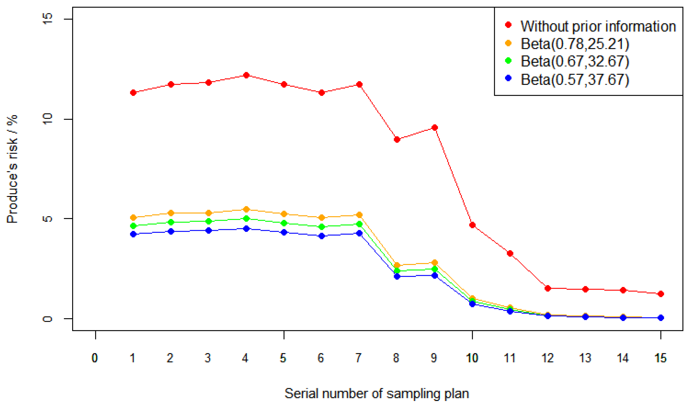
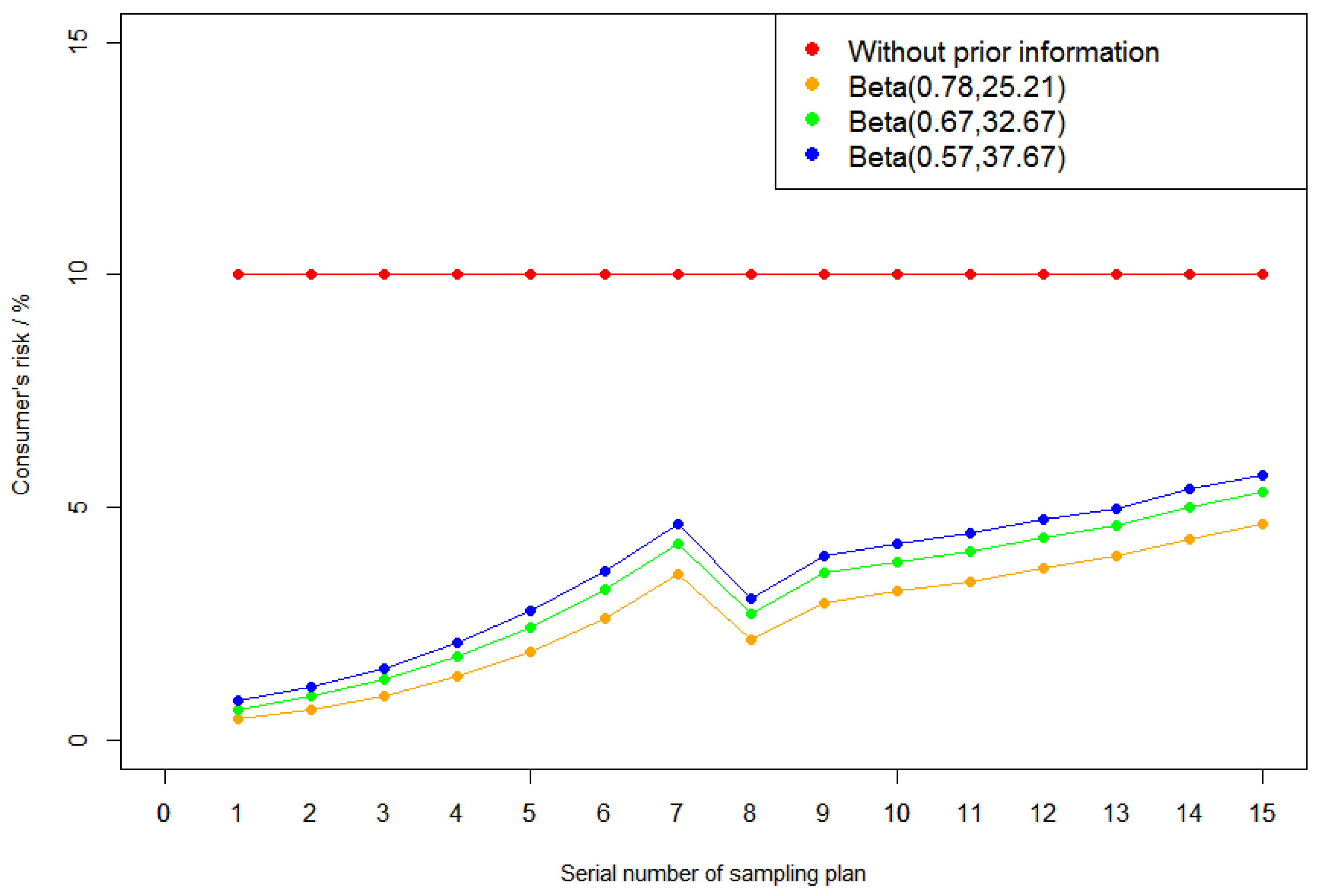
Here we take the different parameter cases with the prior information in Table 2. Without loss of generality, we first consider the first 4 cases in Table 2, and the risk figures of the 15 sampling plans with and without prior information are shown in Figure 1. When the actual quality levels of the lot are the consumer’s risk quality in Table 7, the corresponding consumer’s risk are shown in Figure 2. Consumer’s risk quality in ISO 2859-1:1999 is calculated under assumption that consumer’s risk is 10%, so the consumer’s risks are 10% without prior information in Figure 2.
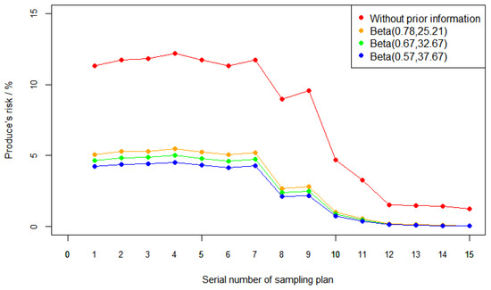
Figure 1.
Producer’s risk figures in different cases. The red line stands for the case without prior information. The other three lines stand for the cases with prior information .
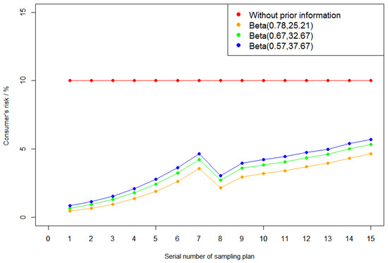
Figure 2.
Consumer’s risk figures in different cases. The red line stands for the case without prior information. The other three lines stand for the cases with prior information .
From Figure 1, we can see the following facts:
- (1)
- When other conditions are given, the producer’s risk trends across the sampling plans in different cases are similar. By and large, the producer’s risk becomes smaller with the increase in AQL and acceptance number c (a larger sampling plans serial number means a larger AQL and acceptance number c);
- (2)
- For all sampling plans, the producer’s risk with prior information is significantly lower than that without prior information;
- (3)
- For the first 10 sampling plan serial numbers (corresponding to the smaller AQL and acceptance number c), the difference in the producer’s risk in different cases is more obvious. This illustrates that prior information is especially important for a small AQL and acceptance number c;
- (4)
- With the decrease in a and the increase in b in the prior information , the nonconforming rate estimated by the prior information is becoming smaller and smaller, and the producer’s risk is becoming lower and lower.
From Figure 2, we can conclude the following:
- (1)
- The consumer’s risks are 10% for all sampling plans without prior information. This is reasonable because our consumer’s risks are calculated at the consumer’s risk quality point. In ISO 2859-1:1999, the consumer’s risk quality is the lot or process quality level, which corresponds to a 10% consumer’s risk in the sampling plan;
- (2)
- The consumer’s risks with prior information are significantly lower than without prior information, especially for a smaller AQL. Therefore, it can be concluded that, when other conditions are given, consumer’s risk considering the prior information for all sampling plans is smaller;
- (3)
- With the decrease in a and the increase in b in the prior information , the nonconforming rate estimated by the prior information is becoming smaller and smaller, and the consumer’s risk is a little bigger.
In summary, for the same sampling plan, the corresponding producer’s and consumer’s risks considering the prior information are smaller compared to no prior information. Especially in the case of smaller AQLs, the decrease is more obvious. There are similar results for the other values of pairs in Table 1, which are omitted here.
4.2. Risk Comparison of Classic Sampling Plan for Different Sample Sizes under Different Prior Information
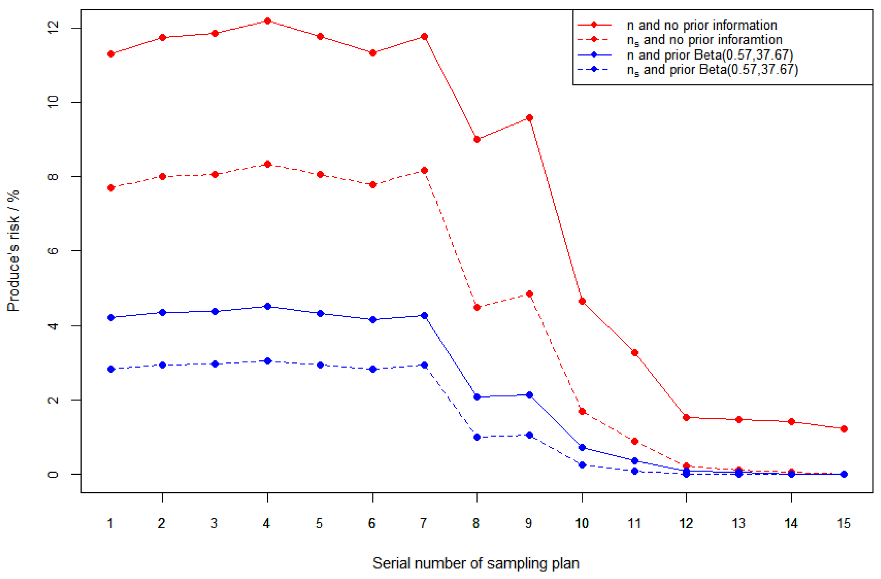
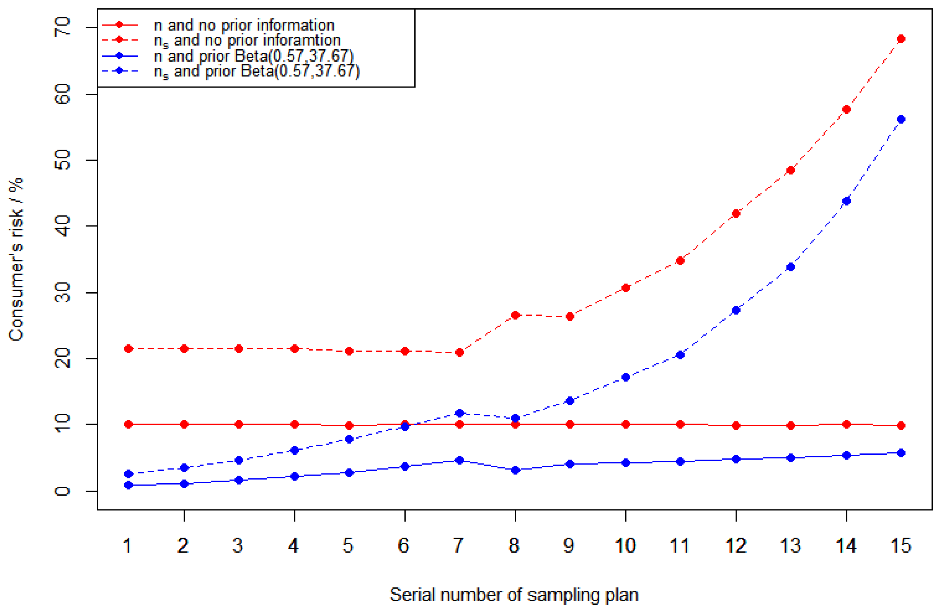
In this section, we consider the effect of sample size on risk with and without prior information. The reference sampling plans are the same as Table 7. For comparison, we change the sample size n to a smaller sample size for every sampling plan in Table 7, while the acceptance number c is the same. The corresponding producer’s risk and consumer’s risk in different cases are shown in Figure 3 and Figure 4.
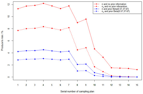
Figure 3.
Producer’s risk figures in different cases. The red line stands for different sample size cases without prior information. The blue line stands for different sample size cases with prior information .
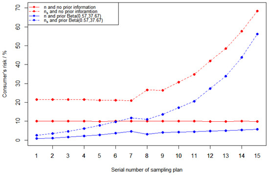
Figure 4.
Consumer’s risk figures in different cases. The red line stands for different sample size cases without prior information. The blue line stands for different sample size cases with prior information .
- (1)
- Regardless of whether there is prior information, the producer’s risk decrease and consumer’s risk increase for different sampling plans as sample size decreases;
- (2)
- In general, the producer’s risk and consumer’s risk with prior information are lower than the corresponding risk without prior information;
- (3)
- In the case with prior information, the reduction in the producer’s risk is greater and the increase in the consumer’s risk is smaller.
These conclusions enable us to be able to design sampling plans with smaller sample sizes by using prior information under the same risk control requirements.
5. Conclusions and Discussions
In this paper, an attribute sampling plan is developed for resubmitted lots based on prior information and Bayesian approach. The new attribute sampling plans adjust sample sizes to prior information based on the status of the inspection target. To be specific, the sampling plans in this paper are indexed in the parameter of trust with levels of low, medium, and high, where increasing trust level reduces sample size or risk. PCIs are an important basis for the choice of the trust level. Let denote the value of PCI. If , this implies that the process capability is not sufficient and that the level of trust is low. If , this implies that the process capability is sufficient and that the level of trust is medium. If , this implies that the process capability is very sufficient and that the level of trust is high. Furthermore, a quality manager who intends to inspect a lot may choose the trust level based on past records of the lot inspection process. In addition, multiple comparisons have been performed, including the producer’s risk and consumer’s risk under different prior information parameters and different sample sizes. However, there are still some limitations in our paper. Firstly, we did not analyze the effect of measurement uncertainty (sampling uncertainty) in attribute sampling. Therefore, this is also an interesting topic related to the research of sampling plans based on prior information considering measurement uncertainty. Secondly, our study focuses on single attribute sampling. Suitably adapted, the same approach can be used for a double sampling plan, which is also one of our future research topics.
Author Contributions
Methodology, J.Z. and F.Z.; Software, F.Z. and X.Z.; writing—review and editing, X.Z. and Y.H.; Supervision, W.D. All authors have read and agreed to the published version of the manuscript.
Funding
This research was funded by the State Administration for Market Regulation Science and
Technology Project (2022MK186) and the China National Institute of Standardization through the
“Special funds for basic R&D undertakings by welfare research institutions” (522022Y-9402).
Data Availability Statement
This maubuscript doesn’t include practical data.
Conflicts of Interest
The authors declare no conflicts of interest.
References
- Balamurali, S.; Gb, R.; Jun, C.-H. Attributes Sampling Schemes in International Standards; John Wiley & Sons, Ltd.: Hoboken, NJ, USA, 2008. [Google Scholar]
- Gb, R.; Baillie, D. Sampling for Nonconformities and Other Issues in the Forthcoming Revision of ISO 2859-2. Qual. Reliab. Eng. Int. 2012, 28, 546–562. [Google Scholar] [CrossRef]
- Klingst, A. Quality Control and Industrial Statistics. Metrika 1959, 2, 253–254. [Google Scholar]
- Schilling, E.G.; Neubauer, D.V. Acceptance Sampling in Quality Control, 3rd ed.; Chapman and Hall/CRC: Boca Raton, FL, USA, 2017. [Google Scholar]
- Zhao, H.; Xu, D. Study and application on sampling test plan of water saving irrigation products based on Bayesian method. Trans. Agric. Mach. 2010, 41, 56–61. [Google Scholar]
- Xiang, B.; Liu, Z. A Sampling Plan of Small Samples for Distribution Network Materials Considering Cost. J. China Three Gorges Univ. Sci. 2022, 44, 83–88. [Google Scholar]
- Khalifa, M.; Khan, F.; Haddara, M. Bayesian sample size determination for inspection of general corrosion of process components. J. Loss Prev. Process Ind. 2012, 25, 218–223. [Google Scholar] [CrossRef]
- Shi, J.X.; Gao, Q.; Liu, H.w.; Xu, L.; Liu, H.W. Design and Application of Sampling Plan Based on Process Capability Index. J. Xi’an Technol. Univ. 2019, 39, 750–754. [Google Scholar]
- He, Q. Study of the Variables Sampling Inspection Scheme Based on the Process Capability Index; Yanshan University: Qinhuangdao, China, 2014. [Google Scholar]
- Seifi, S.; Nezhad, M.S.F. Variable sampling plan for resubmitted lots based on process capability index and Bayesian approach. Int. J. Adv. Manuf. Technol. 2017, 88, 2547–2555. [Google Scholar] [CrossRef]
- Sherman, R.E. Design and Evaluation of a Repetitive Group Sampling Plan. Technometrics 1965, 7, 11–21. [Google Scholar]
- Pearn, W.L.; Wu, C.W. An effective decision making method for product acceptance. Omega 2007, 87, 29–41. [Google Scholar] [CrossRef]
- von Collani, E.; Dumitrescu, M.; Lepenis, R. Neyman measurement and prediction procedures. Econ. Qual. Control 2001, 16, 109–132. [Google Scholar] [CrossRef]
- Hald, A. Statistical Theory of Sampling Inspection by Attributes; Academic Press: London, UK, 1981. [Google Scholar]
- Godfrey, J.T.; Andrews, R.W. A finite population Bayesian model for compliance testing. J. Account. Res. 1982, 20, 304–315. [Google Scholar] [CrossRef]
- Berg, N. A simple Bayesian procedure for sample size determination in an audit of property value appraisals. Real Estate Econ. 2006, 34, 133–155. [Google Scholar] [CrossRef]
- Corless, J.C. Assessing Prior Distributions for Applying Bayesian Statistics in Auditing. Account. Rev. 1972, 47, 556–566. [Google Scholar]
- Walls, L.; Quigley, J. Building Prior Distributions to Support Bayesian Reliability Growth Modeling Using Expert Judgment. Reliab. Eng. Syst. Saf. 2001, 74, 117–128. [Google Scholar] [CrossRef]
- Blocher, E.; Robertson, J.C. Bayesian Sampling Procedures for Auditors: Computer-Assisted Instruction. Account. Rev. 1976, 51, 359–363. [Google Scholar]
- Garthwaite, P.H.; O’Hagan, A. Quantifying Expert Opinion in the UK Water Industry: An Experimental Study. J. R. Stat. Soc. Ser. (Stat.) 2000, 49, 455–477. [Google Scholar] [CrossRef]
- ISO 2859-1; Sampling Procedures for Inspection by Attributes-Part 1: Sampling Schemes Indexed by Acceptance Quality Limit (AQL) for Lot-by-Lot Inspection. International Organization for Standardization: Geneva, Switzerland, 1999.
- Johnson, J.R.; Leitch, R.A.; Neter, J. Characteristics of errors in accounts receivable and inventory audits. Account. Rev. 1981, 56, 270–293. [Google Scholar]
- Ham, J.; Losell, D.; Smieliauskas, W. An empirical study of error characteristics in accounting populations. Account. Rev. 1985, 60, 387–406. [Google Scholar]
- Gob, R.; Uhlig, S.; Colson, B. Conformity assessment of processes and lots in the framework of JCGM 106:2012. Available online: https://sd.iso.org/documents/ui/browse/iso (accessed on 23 May 2024).
Disclaimer/Publisher’s Note: The statements, opinions and data contained in all publications are solely those of the individual author(s) and contributor(s) and not of MDPI and/or the editor(s). MDPI and/or the editor(s) disclaim responsibility for any injury to people or property resulting from any ideas, methods, instructions or products referred to in the content. |
© 2024 by the authors. Licensee MDPI, Basel, Switzerland. This article is an open access article distributed under the terms and conditions of the Creative Commons Attribution (CC BY) license (https://creativecommons.org/licenses/by/4.0/).