Abstract
Imaging hyperspectral technology is becoming popular in agriculture to provide detailed information on crop growth. In this work, we propose an estimation of rapeseed pod’s water content model and identification of maturity levels (green, yellow, and full) model by using this technology. Four types of hyperspectral features are extracted—color, texture, spectral three-edge parameters, and spectral indices. By integrating these features, satisfactory results are achieved: the optimal feature combination is from spectral indices and three-edge parameters, with low RRMSE and RE for yellow maturity. Incorporating spectral indices significantly improved the pod’s water content estimation, reducing RRMSE by up to 43.30% and 30.11% in the green and full maturity stages. Random forest and support vector machine with kernel method (SVM-KM) algorithms outperformed other statistical models, with SVM-KM achieving up to 96.90% accuracy in identifying maturity levels. These findings provide valuable insights for managing rapeseed production during the pod stage.
MSC:
62H30; 62J10; 62F05
1. Introduction
As a pivotal oilseed crop, rapeseed (Brassica napus L.) has garnered substantial research interest in agricultural sciences, particularly pertaining to growth regulation and yield/quality enhancement. The pod-filling stage is a critical determinant of seed production [1], with approximately two-thirds of the dry matter accumulation attributed to photosynthesis in the pod [2]. Notably, during the green-ripe and yellow-ripe phases of pod development, photosynthetic efficiency exhibits a strong correlation with the water status of the pod. Consequently, precise monitoring of the pod’s water content during these stages is imperative. However, as pods mature, pod shatter emerges as a prevalent issue, adversely impacting harvest efficiency and yield. Inadequate harvest timing management can result in up to 20% yield losses [3]. Since the pod’s water content and maturity level are key factors influencing pod shatter susceptibility [4,5,6,7,8], they provide valuable insights for optimizing harvest timing and mitigating losses. In summary, the capacity for rapid, non-destructive detection of rapeseed pod’s water content and accurate identification of maturity stages is crucial for maximizing yield and quality in rapeseed production systems.
Traditional desiccation-based techniques for quantifying rapeseed pod pericarp water content [9,10,11] are not only time-consuming and labor-intensive but also destructive, precluding their effective integration with remote sensing technologies for rapid and accurate assessment across large-scale cultivation areas. Conventionally, the determination of optimal harvest timing has heavily relied on empirical observations, such as the visual cue of field-wide pod yellowing resembling loquat fruits or pericarp water contents ranging between 11 and 13% [12]. However, these subjective approaches lack consistency, are challenging to master, and are antithetical to the principles of smart agriculture. Consequently, the development of rapid, non-destructive methodologies for estimating rapeseed pod pericarp water status and maturity is a critical imperative for optimizing yield and quality in rapeseed production systems.
Imaging hyperspectral technology offers a viable solution by synergistically combining imaging and spectroscopic modalities, facilitating the simultaneous acquisition of spatial and biochemical information from target specimens. This integrative approach has emerged as an invaluable diagnostic tool for plant phenotyping and growth monitoring. In recent years, numerous studies have leveraged hyperspectral imaging to assess plant physiological status through spectral information analysis [13,14,15,16,17,18], with a burgeoning focus on water content determination [19,20,21,22,23,24], such as Sun et al. [22] who developed a hyperspectral method for accurate, rapid lettuce leaf water content detection during growth. Applying the CARS-ABC-SVR model optimized using an artificial bee colony algorithm, the R2 is found to be 0.9214 and the RMSE is 2.95% on the prediction set.
Spectral data are information-rich, but the strong correlations and redundancies among adjacent frequency bands may impact efficiency and accuracy [25,26,27]. Image data facilitate target recognition and estimation through color and texture features, providing multi-angular information. To obtain comprehensive and refined target information from raw imaging hyperspectral data, feature extraction and inter-class feature fusion are required. This approach overcomes single-data modality limitations, fully leverages the complementarity of multi-angular and multi-dimensional information, and enhances decision-making accuracy and reliability. Peñuelas et al. [28] constructed the Water Band Index (WBI) using the 970 nm water-sensitive waveband and the 900 nm reflectance, verifying WBI’s effectiveness in predicting leaf water stress. Ramoelo et al. [29] demonstrated the practicality of field spectroscopy for estimating nitrogen-to-phosphorus ratios in savanna grasses. Zhang et al. [30] extracted feature parameters from rapeseed canopy spectra, multispectral images, and canopy temperature, constructing an information fusion estimation model for rapeseed water content, exhibiting significantly higher accuracy than single-modality models.
In this work, we apply imaging hyperspectral features to investigate water content estimation and maturity level identification, which are of importance to rapeseed pod production management. Four types of features including color, texture, spectral three-edge parameter, and spectral index are extracted from hyperspectral data. These features are then combined intra-class and fused inter-class. Multiple machine learning models are employed to model for the purpose mentioned above.
2. Materials and Methods
2.1. Experimental Materials
For this experiment, we selected the Fengyou 520 rapeseed cultivar bred by the Hunan Crop Research Institute. The plants were planted in suitable and uniform experimental fields on 2 October 2022. With an average plant height of 167.6 cm, this cultivar belongs to the mesophytic branching type. We collected samples during three critical periods of pod development: Pod Stage I or Green Ripe Stage (where pods are initially formed and appear full, 18 April 2023, denoted as P1), Pod Stage II or Yellow Ripe Stage (where pods start to turn yellow in small areas, 28 April 2023, denoted as P2), and Pod Stage III or Full Ripe Stage (where most of the pods are yellow and maturing, starting to dry gradually, 23 May 2023, denoted as P3). To avoid weather influences like rainfall or morning and evening dew, we collected samples in the afternoon of the third consecutive sunny day when the field temperature was between 20 °C and 25 °C. Each time, we randomly selected 8 rapeseed plants from the experimental area and picked 9 pods from each plant: 1 pod each from the top 0–20 cm, 20–40 cm, and 40–60 cm sections, and 1 pod each based on color shade (greenish, yellow-green, and yellowish). Immediately after sampling, the pods were taken to the laboratory for imaging hyperspectral and water content measurement. In this way, 216 pod samples were collected across the three stages.
2.2. Data Acquisition and Processing
2.2.1. Data Acquisition
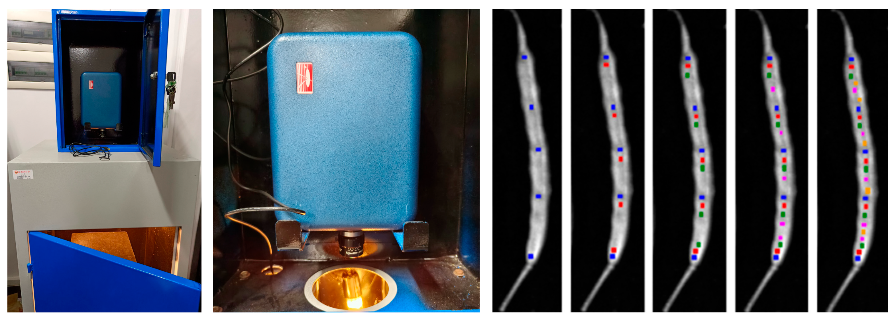
In this work, a SOC710 hyperspectral imager (wavelength 375–1041 nm, resolution 4.6875 nm, produced by Surface Optics Co., 11555 Rancho Bernardo Road San Diego, California 92127, USA) was used to measure imaging spectral data, as shown in Figure 1. The experiment was conducted in a darkroom using a 50 × 60 cm, 100 cm high mission module coated with diffuse reflective material, surrounded by a 70 W halogen light source at a 45-degree angle, and equipped with a ventilation and cooling system. The imager was placed vertically above the target with an exposure distance of 300 mm. After preheating for 15 min, the imaging spectral information of the rapeseed pods was measured. Data processing was performed using Spectral Radiance Analysis Toolkit and ENVI5.3 software, and 5 rounds of random measurements were taken in the region of interest of the pods, with the average value taken as the final spectral reflectance value of the ROI.

Figure 1.
Experimental mission module (left), SOC710 hyperspectral imager (middle), and ROI of reflectance samples (right). The five blue square-shaped points are the first round of random measurements, which were taken in the ROI of a pod, with the average value taken as the first spectral reflectance value. The red, green, pink and orange represent the second, third, fourth, and fifth round of selection, respectively. The average of the five rounds is averaged as the final spectral reflectance value of the ROI.
On the other hand, we employed a high-precision TP300D electronic balance and a 101-type electric heating blowing dry box to measure the water content of the pod pericarp. The balance has a range of 300 g, an accuracy of 0.001 g, and multiple functions such as calibration, peeling, and zero tracking. The temperature control range of the drying box is 5–250 °C, the temperature control accuracy reaches ±1 °C, and the temperature uniformity is 3.5%, which is accurate and easy to maintain. After obtaining the imaging hyperspectral data of rapeseed pods, to avoid the influence of oil volatilization in rapeseed on the measurement results, we performed seed removal on the pods before each drying. After a series of operations such as seed removal, weighing the fresh weight of the pod pericarp, drying the pod pericarp to a constant weight, and weighing the dry weight, the water content of the pod pericarp was calculated. We obtained a total of 216 data points for pod pericarp water content. Table 1 lists the statistical characteristics of water content in rapeseed pod pericarp at various stages in detail. As can be seen from the table, there is little difference in the mean water content between the green and yellow maturity stages, while the mean water content during the full maturity stage is significantly reduced, and the coefficient of variation is significantly increased. Through the above process, we obtained a total of 216 spectral reflectance curves and the corresponding RGB images, as well as the pod’s water content.

Table 1.
Statistical characteristics of pod’s water content.
2.2.2. Feature Extraction
To avoid data redundancy and improve modeling efficiency, four types of features of the imaging hyperspectral data are extracted for our consideration, namely image color, image texture, spectral three-edge (red, blue, yellow) parameters, and spectral index.
- Image color
Focusing on the region of interest after eliminating background interference in the hyperspectral images of rapeseed pods, we obtained 98 color features according to the ten-color method [31,32,33]. Those color features are labeled as “TcC-” prefix.
- Image texture
Texture features reveal changes in the image surface and the organizational characteristics of its structure. Based on the rapeseed pod images, various texture features, such as contrast, energy, correlation, entropy, third-order moments, brightness, consistence, homogeneity, and smoothness are extracted through the gray-level co-occurrence matrix [34], which are labeled as “TcT-” prefix, as listed in Table 2.
Table 2.
The calculation formula of image texture features.
- Spectral three-edge parameter
The red edge parameters refer to the reflection spectral characteristics of green plants in the red edge (680–760 nm), including red edge position, red edge amplitude, and red edge area. Additionally, the blue edge (490–530 nm) and yellow edge (560–640 nm) parameters, collectively known as spectral three-edge parameters [32,35], are related to the growth status and biomass of plants. We choose 23 three-edge parameters for our consideration, which are identified with the “Tri-” prefix, as listed in Table 3.
Table 3.
The calculation formula of hyperspectral three-edge parameters.
- Spectral index
The crop spectral index is the feature obtained by combining spectral reflectance from sensitive wavelength regions, which is very useful for assessing and monitoring crop growth. Ratio spectral index (RSI), normalized difference spectral index (NDSI), and difference spectral index (DSI), which are most important for green crops [36], are used for our study. In addition, four other key spectral indices related to plant water content, namely plant senescence reflectance index (PSRI) [37], ripening stage of pod maturity index (RSMI) [38], structure-independent pigment index (SIPI) [39], and modified normalized difference red edge index (mNDRE) [37], are also employed. The calculation formulas are shown in Equations (1)–(7), where Rλ1, Rλ2, and Rλ3 represent the reflectance at wavelengths λ1, λ2, and λ3, respectively, which are labeled as “SpI-” prefix. Considering the differences in sensitive bands of spectral indices among different crops and varieties, we perform interactive combinations of bands in the range of 375–1041 nm. According to the correlation analysis with the pod’s water content, the wavelength bands with the highest correlation coefficient are obtained at the three periods, listed in Table 4, Table 5 and Table 6.
Table 4.
The top three features corresponding to the best correlation coefficient (CC) in P1.
Table 5.
The top three features corresponding to the best correlation coefficient (CC) in P2.
Table 6.
The top three features corresponding to the best correlation coefficient (CC) in P3.
The color and texture features in imaging hyperspectral provide information about color differences and spatial distribution of the samples. The spectral index reflects characteristics derived from combinations of different bands in hyperspectral reflectance, while spectral three-edge parameters describe the hyperspectral performance at potentially sensitive locations. Therefore, various features may contribute to better model performance, to some extent, in estimating the pod’s water content.
2.3. Feature Fusion and Modeling
2.3.1. Feature Fusion
By using raw data and its feature information as training datasets for machine learning algorithms, information fusion can be achieved, bringing many advantages such as improving estimation accuracy, enhancing feature expression, and improving model stability and interpretability. Information fusion can be classified into three types based on the level of processing: data-level fusion, feature-level fusion, and decision-level fusion [42]. In this work, a feature-level fusion strategy is adopted. Firstly, the correlation analysis is conducted between each type of feature introduced above and the pod’s water content. Three features with the highest correlation are selected for each category, followed by an intra-class combination (CB) and inter-class fusion (FS) processing of these features. CB-TcC{*,*,*}, CB-TcT{*,*,*}, CB-SpI{*,*,*}, and CB-Tri{*,*,*} represent the intra-class combinations of the four types of features, respectively. Inter-class feature fusion is represented by FS{*,*,… }; for example, FS{CB-SpI, CB-Tri} denotes the deep fusion of the spectral index and three-edge parameters, in which there are six features.
2.3.2. Modeling Methods and Processes
Random decision forest (RDF) is a highly integrated supervised learning algorithm that utilizes decision trees as estimators [43]. Decision trees are constructed from randomly selected subsets of data and features, and classification results are obtained through bagging resampling and a voting mechanism, suitable for both classification and regression problems. The RDF model is flexible in structure, strong in fault tolerance, and easy to understand and implement [44]. We use the RDF to build an estimation model of the pod’s water content, and a recognition model of the pod’s maturity levels. Meanwhile, the effects of other modeling methods, such as linear regression, support vector machines, and neural networks are compared. The modeling process is presented in Figure 2.
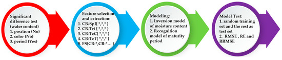
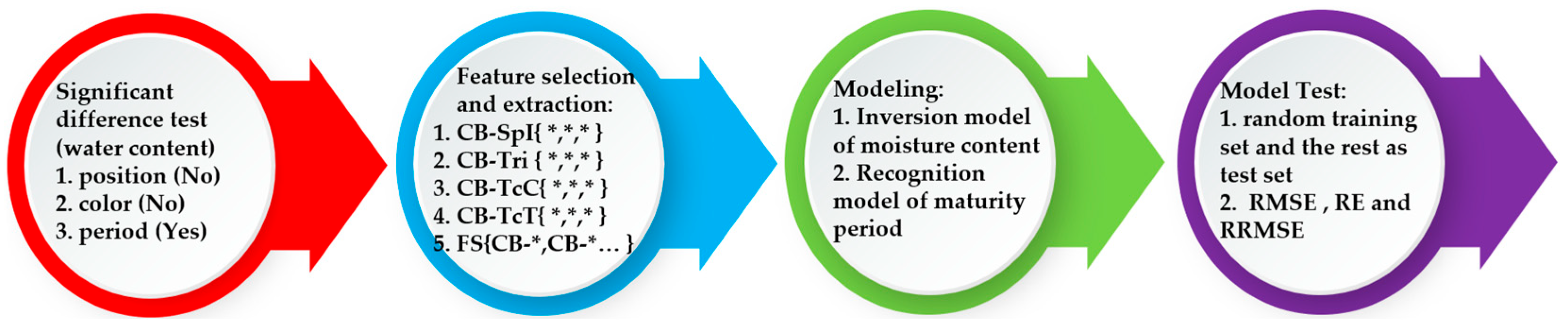
Figure 2.
Modeling process diagram.
According to the diagram, we execute the tasks of the pod’s water estimation modeling and maturity identification modeling in four steps.
- Step 1:
- Significance analysis
Firstly, we conduct variance analysis on the pod’s water content samples from different periods, positions, and colors. The results show that the water content was significantly affected only by the period, while the three positions and three colors had no significant difference in their effects on water content. Based on this finding, we decided to use spectral data only for period classification and recognition.
- Step 2:
- Feature extraction and data fusion
Next, we select the three most correlated feature parameters from each of the four feature categories through correlation analysis with the water content of the silique pericarp. We then form intra-class combinations (CB-*{*,*,…}) and inter-class fusion combinations (FS{CB-*, CB-*…}) as inputs for subsequent models.
- Step 3:
- Model Construction
Based on various feature combinations, we fuse the extracted feature data using machine learning algorithms. By comparing evaluation metrics from 100 model runs, we establish a quantitative model to invert the pod’s water content. Targeting different pod’s maturity periods, we use the coefficient of variation Io to select the most sensitive features from spectral indices, color, texture, and spectral parameters.
- Step 4:
- Model Validation and Optimization
Finally, we test the accuracy and stability of both the pod’s water content inversion model and the pod’s maturity recognition model by varying the number of training set samples with K-fold cross-validation.
2.3.3. Model Evaluation
In this paper, root mean square error (RMSE), relative error (RE), and relative root mean square error (RRMSE) are adopted as metrics to evaluate the modeling results. Among them, RMSE can effectively reflect the accuracy of the estimation model. The closer its value is to 0, the higher the estimation accuracy of the model. RE measures the absolute error ratio between the measured value and the true value, and a smaller RE value indicates smaller errors. RRMSE, defined as the ratio of RMSE to the average value of the target variable and expressed as a percentage, can eliminate the influence of dimensions on the evaluation results [45]. The formulas are as follows:
3. Results and Discussion
3.1. Significant Difference Test of Pod’s Water Content
The pod samples were picked from three growth locations (see Section 2.1) at three color levels. To detect whether there is a difference in the water content of pods under these two factors, analysis of variance (ANOVA) is conducted at the three periods (P1, P2, P3) as well as the whole period (PW) of the pods. We listed the statistical p-values in Table 7. Clearly, during the periods of P1, P2, and P3, both position and color have no significant effect on the pod’s water content. The potential reasons may be (1) in the P1, the vascular bundle structure inside the rape stalks is intact and elastic at this stage, allowing normal transport of water and nutrients. (2) In the P2, though the pods begin to turn yellow, the pods are not fully ripe yet. The stalks still retain their toughness and the vascular bundles function normally, thus pods in different positions and colors still have normal water absorption capabilities. (3) In the P3, the rape seeds are completely mature, and the pods turn completely yellow and gradually dry. Although the stalks show signs of aging, such as slight lignification or color changes, the water and nutrient transport capacity of the vascular bundles may be somewhat reduced. However, they are still relatively intact and not sufficient to significantly affect the water content of different pods.
Table 7.
Significant p-value of pod’s water content for different pod positions, color combinations, and their interactions.
ANOVA between periods shows that the pod’s water content is significantly affected by the growth stage. In this regard, we focus on the pod’s water content modeling in each period and ignore the influence of pod position and color.
3.2. Correlation Analysis
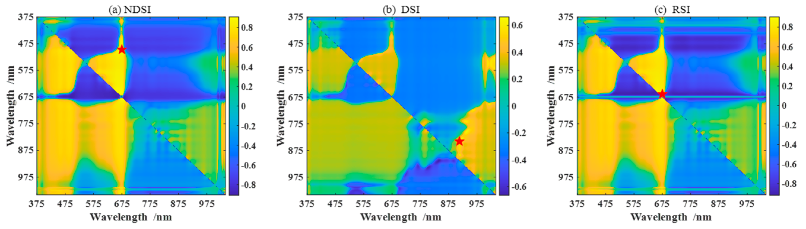
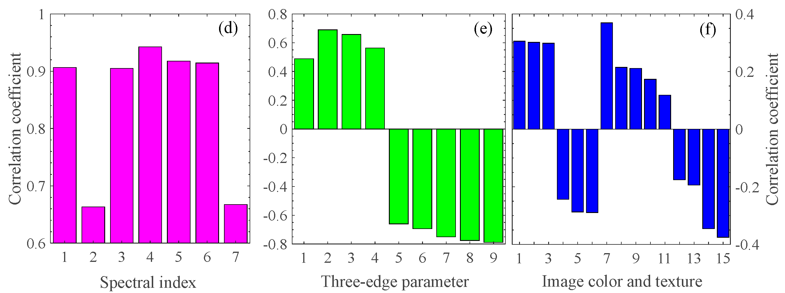
To select feature parameters to estimate the pod’s water content, we perform the correlation analysis between the pod’s water content and the various feature parameters. Figure 3a–c are heatmaps of the correlation coefficients between any two-band combinations of NDSI, DSI, and RSI spectral index (given by Equations (1)–(3)) in the range of 375–1041 nm and the pod’s water content at P1. The deeper the color, the higher the degree of correlation. The red pentagram corresponds to the maximum correlation coefficient. In addition, the other four spectral indices, PSRI, RSMI, SIPI, and mNDRE (given by Equations (4)–(7)), are also studied. Figure 3d shows the correlation coefficients between the optimal band combinations of seven spectral indices and the pod’s water content. The top three are PSRI, RSMI, and SIPI, with correlation coefficients of 0.9425, 0.9178, and 0.9146, respectively. Meanwhile, the nine spectral three-edge parameters are also performed in the correlation analysis, as shown in Figure 3e. Among them, NDBE, NDYE, and NDRE have the highest correlation with the water content, with the correlation coefficients −0.7888, −0.7756, and −0.7506, respectively. Figure 3f shows the correlation of the top six image colors and all image textures within the pod’s water content. Table 4 shows the top three feature parameters with the best correlation of the above four types of features during P1. Similarly, the top three features corresponding to the best correlations in P2 and P3 are shown in Table 5 and Table 6, respectively. In what follows, we use these feature parameters as feature combinations or fusions to establish models for estimating the pod’s water content.
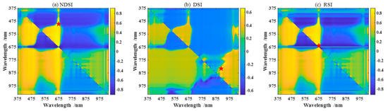

Figure 3.
Correlation analysis between four types of features and the pod’s water content. (a–c) The three main spectral indices (NDSI, DSI, and RSI); The red pentagram represent the coordinates of the two wavelengths corresponding to the maximum correlation coefficient. (d) The seven spectral indices; the number represents NDSI, DSI, RSI, PSRI, RSMI, SIPR, and mNDRE in order. (e) The nine spectral three-edge parameters with the absolute value of correlation coefficient larger than 0.4; the number represents Drmin, BR, YR, BY, NRY, NRB, NDRE, NDYE, and NDBE in order, described in Table 3. (f) The six image colors with the absolute value of correlation coefficient larger than 0.2, and nine image texture features; the number represents (2G-R-B)/L*, G-R, G/Y, B-Y, R-Y, a*, contrast, smoothness, average brightness, entropy, third-order moments, consistence, energy, correlation, and homogeneity in order.
3.3. Pod’s Water Content Estimation Modelling
3.3.1. Analysis and Comparison of the Estimation Model in P1
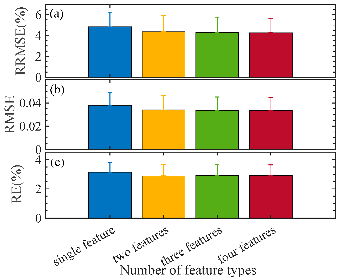
An estimation model for the pod’s water content in P1 is established using the RDF algorithm. In total, 56 samples are randomly selected as the training set, while the remaining samples serve as the test set. The pod’s water content is set as the output layer, and the combined/fused features are used as the input layer. According to Table 4, those three features in identical types are combined, and two, three, or four combinations are fused (denoted as FS{CB-*,CB-*,…}). To eliminate the influence of random factors, 100 repetitions are conducted. The results are obtained on the test set, which are listed in Table 8. Figure 4 illustrates RRMSE, RMSE, and RE, as well as their standard deviations under the best feature combination/fusion. The results indicate that multi-category fusion is superior to single-category combination. As the number of feature categories increases, the overall trend of various indicators decreases and the standard deviation also decreases. It suggests that the accuracy and stability of the model improve as the number of feature parameter categories increases. However, the trend of model optimization slows down when the number of fusion combination categories reaches two or more. To confirm this, a T-test is implemented for them, and the statistical p-value is listed in Table 9. The fusion effect by two types of features is significant. In contrast, there is no significant difference between more feature fusions. In this regard, we suggest the two types of feature fusion FS{CB-SpI, CB-Tri} for the pod’s water content modeling for the sake of modeling efficiency. The RRMSE, RMSE, and RE are 4.3458%, 0.0340, and 2.8841%, respectively. To test the performance of the RDF, we also apply other five statistical models for the same purpose; the results are obtained on the dual feature fusion FS{CB-SpI, CB-Tri}, also listed in Table 8.
Table 8.
Performance of modeling on the pod’s water content with respect to various feature combinations in P1. The best result of each case is in bold.
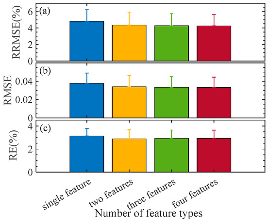
Figure 4.
RRMSE, RMSE, and RE with different fused features. Error bar indicates the standard deviation from the 100 repetitions. (a–c) are the variation of RRMSE, RMSE, and RE with the number of feature types, respectively.
Table 9.
T-test of statistical p-values of feature fusion in P1.
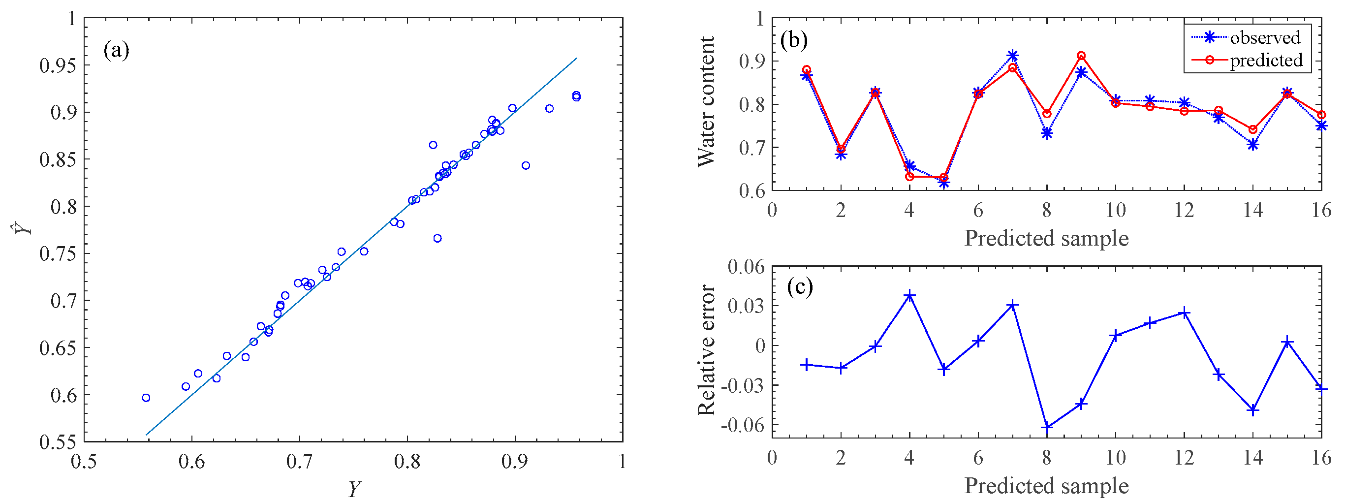
We show the RDF model performance under the two types of features fusion FS{CB-SpI, CB-Tri} in P1 in Figure 5. The left panel illustrates the fitted and observed values of the pod’s water content on the training set. The right panels compare the observed and estimated water content values on the testing set.

Figure 5.
Model performance under the two types of features fusion. Left is on the training set and right is on the testing set. (a) is the result from the training set (56 samples). The right panel is the resuIts on the test set (remaining 16 samples), where (b) is the relative error, and (c) is the comparison between the observed and predicted water content values.
To further investigate the influence of spectral index and spectral three-edge parameters on the model performance, we compare the results that include these features with those that do not, as listed in Table 10. It is observed that the spectral index and spectral three-edge parameters indeed have a significant positive effect on the model. By comparison, the former demonstrates a better performance than the latter.
Table 10.
Influence of the spectral index and spectral three-edge parameters on model performance in P1 (the best result of each case is in bold).
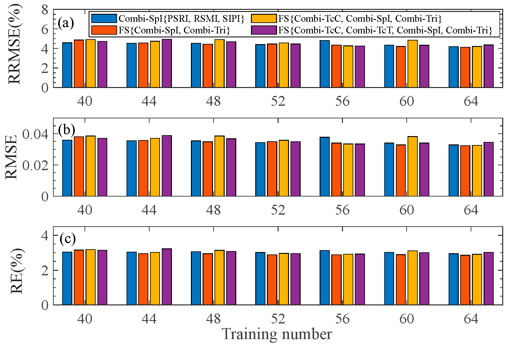
To evaluate the stability of the pod’s water content estimation model, we vary the number of samples in the training set, i.e., the number of samples is set from 40 to 64 with random selection. The average results of the three evaluation indicators (RRMSE, RMSE, and RE) are calculated, as shown in Figure 6. It is found that there is no significant change with an increase in the training set size, indicating that the selected fused feature exhibits satisfactory stability.
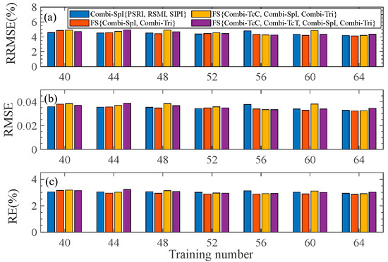
Figure 6.
RRMSE, RMSE, and RE of the test set with respect to the training number under different types of feature fusion. (a–c) are for the fluctuation of RRMSE, RMSE, and RE, respectively.
3.3.2. Analysis and Comparison of Estimation Models for P2 and P3
The pod’s water content modeling in P2 and P3 is conducted similarly to P1. Table 11 lists the optimal single-feature combinations and two types of feature fusions. The optimal two types of feature fusions in P2 and P3 remain the same as in P1, i.e., FS{CB-SpI, CB-Tri}. However, the optimal feature combination differs between the three periods. For P2, the best RRMSE, RMSE, and RE are 2.6218%, 0.0212, and 1.8820%, respectively. For P3, the RRMSE, RMSE, and RE are 34.1718%, 0.0758, and 25.0430%, respectively. The poor model performance in P3 is due to the very low water content of the pods, which cannot be accurately identified by existing instruments. It is necessary to continuously improve the resolution and other performances of the experimental equipment. Additionally, further research is needed to expand the spectral band range, innovate more effective feature extraction methods, and develop new modeling approaches, which are the directions for future exploration.
Table 11.
Optimal feature combination/fusion in the three pod stages.
3.4. Recognition Model for Pod’s Maturity Level
3.4.1. Analysis of Recognition Models
Recognizing the maturity level of rapeseed pods can help determine the growth status of rapeseed and the optimal harvest timing, preventing low grain weight and oil content caused by premature harvesting, or pod cracking, grain and oil content loss caused by late harvesting. Therefore, accurately judging the maturity level of rapeseed pods and determining the appropriate harvest time can help managers arrange farming activities reasonably and improve efficiency.
Based on the significant difference test for the pod’s water content presented in Section 3.1, it is evident that the water content is primarily influenced by the pod’s different growth stages. To intelligently distinguish the maturity level of the pods, we extract the features by referencing sensitive characteristics of entire pod growth stages from the imaging hyperspectral data first. This resulted in 151 features, namely 16 spectral indices, 27 spectral three-edge parameters, 98 image color features, and 10 image texture features for 216 pod samples. To improve efficiency during modeling, an indicator Io, similar to the variation coefficient, is proposed to screen the optimal features. On the one hand, let σi represent the standard deviation of feature values among 72 samples in period Pi (i = 1, 2, 3), characterizing the intra-period difference. Marking the average value over the three periods as . On the other hand, σa denotes the standard deviation of the average value of the studied feature across the three periods, indicating inter-period difference. The indicator Io is the ratio of these two standard deviations. A smaller Io indicates that the feature parameters selected using this variation coefficient are more effective in distinguishing between periods. The formula is as follows:
Accordingly, we screen the features with the smallest Io from each type of feature, as listed in Table 12. We combine the former three features to construct three-dimensional parameter space {SpI-RSMI, TcC-a*/b*, Tri-NDBE}, as shown in Figure 7, where each point represents a pod’s sample, and different shape symbols denote different pod growth stage. Obviously, the samples of the same period are clustered together, while those from the different periods are well separated.
Table 12.
Ranking of Io for various types of features.
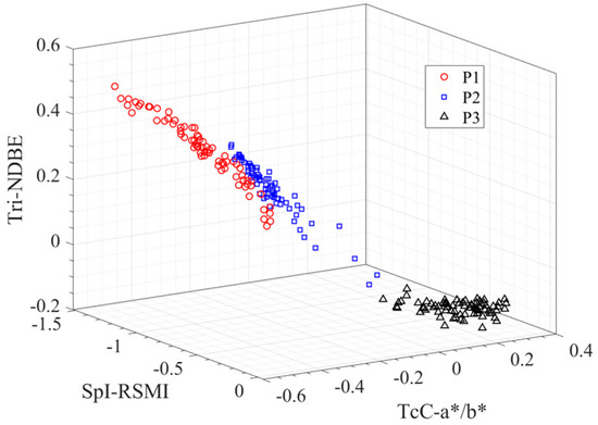
Figure 7.
Visualization of pod samples in three-dimensional space constructed by {SpI-RSMI, TcC-a*/b*, Tri-NDBE}.
Subsequently, the combined features {SpI-RSMI, TcC-a*/b*, Tri-NDBE} are used as inputs for the recognition model. Here, besides the RDF model used for the pod’s water content estimation, we employ two other prevail classification algorithms in machine learning for the recognition model, namely support vector machine and kernel method (SVM-KM) and K-nearest neighbor (KNN). For these algorithms, RDF excels in handling high-dimensional data and feature selection [46], SVM performs well in both linear and nonlinear classification problems [47,48], and KNN has advantages in certain applications due to its simplicity and instance-based learning approach [49]. We adopt K-fold cross-validation to test our model, where (K − 1)/K × 100% of the samples are set as the training set and the ones remaining are in the testing set. By setting K = 2, 4, 6, 8, and 10, the average recognition accuracy for identifying pod periods is obtained, as shown in Table 13. The best recognition effect is achieved using SVM, with 96.90% accuracy. The average modeling accuracy obtained with K = 2–10 ranges from 95% to 97%, demonstrating the good accuracy and stability of the model in recognizing pod periods.
Table 13.
Average accuracy (%) of the three models on {SpI-RSMI, TcC-a*/b*, Tri-NDBE} under K-fold cross-validation.
3.4.2. Model Validation
To demonstrate the effectiveness of the indicator of Io, we randomly choose three other features to combine the three-dimensional features for comparison, namely {SpI-SIPI, TcC-G/Y, Tri-NDRE}, {SpI-SIPI, TcC-(2G-R-B)/L*, Tri-D_rmin}, and {SpI-mNDRE, TcC-DGCV, Tri-NDYE}. Using the SVM-KM algorithm as the classifier, the modeling process is the same as above. The average accuracy is listed in Table 14. Clearly, the optimal feature parameter combination {SpI-RSMI, TcC-a*/b*, Tri-NDBE} selected by Io has the highest accuracy in period recognition.
Table 14.
Average accuracy (%) on different feature combinations under K-fold cross-validation.
Finally, we investigate the impact of the number of features on the modeling results. SVM-KM and 5-fold cross-validation are used for this purpose. The number of features from 1 to 10 is varied, which is selected from the ascending order of the indicator Io. Figure 8 reports the result. The average accuracy arises sharply when the feature number is from 1 to 3; however, it remains almost unchanged when the number of features exceeds 3. Considering the modeling performance and efficiency, we suggest using the three feature combinations {SpI-RSMI, TcC-a*/b*, Tri-NDBE} for recognition modeling of the pod growth stage.
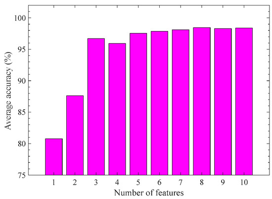
Figure 8.
Average recognition accuracy of pod periods with different numbers of features based on SVM-KM.
4. Discussion and Conclusions
In this paper, imaging spectrometry technology is utilized to construct inversion models for water content in rapeseed pod pericarp and recognition models for pod’s maturity. By fusing features such as image color, texture, spectral three-edge parameters, and spectral indices, it is found that the inter-class feature fusion exhibits higher accuracy and stability in modeling compared to the intra-class feature combination. The best performance is achieved with the inter-class feature fusion combination of FS{CB-SpI, CB-Tri} in all periods. Meanwhile, spectral indices significantly enhance the model’s performance. When establishing the recognition model, variance analysis is employed, and a difference index Io is defined to filter features, resulting in the optimal feature combination of {SpI-RSMI, TcC-a*/b*, Tri-NDBE}. Finally, it is observed that the random forest algorithm performs better in modeling the estimation problems studied in this paper, while the support vector machine algorithm excels in recognition problems. These results provide meaningful references for managing photosynthetic efficiency measures during the pod stage of rapeseed and formulating and implementing low-loss harvesting and drying practices.
It is important to highlight that our focus has been on providing reliable feature selection and interpretable model construction for estimating the pod’s water content and identifying the pod’s maturity. To this end, we conducted thorough feature engineering and machine learning modeling processes.
Existing studies on rapeseed pod’s maturity level recognition or water content estimation are limited. In the existing works [37,38], the authors proposed novel spectral indices, the Canola Pod Maturity Index (CPMI) and Rape Siliques Maturity Index (RSMI), respectively. While the CPMI exhibited satisfactory model performance for canola [37], its correlation with the water content of our rapeseed pods was poor. The RSMI, proposed in [38] and designed for Chinese rapeseed pod cultivars, demonstrated a good correlation coefficient for our data. Consequently, we employed RSMI (given by Equation (5)) as a feature for our modeling. This finding highlights the significant regional differences in rapeseed materials, manifested as variations in optimal spectral indices. In light of the global importance of rapeseed materials, the models proposed in this work can provide valuable experience for subsequent related research.
Author Contributions
Conceptualization, Z.Z. and G.L.; methodology, Z.Z.; software, Z.Z.; validation, Z.Z.; formal analysis, Z.Z.; investigation, Z.Z.; resources, G.L.; data curation, Z.Z.; writing—original draft preparation, Z.Z.; writing—review and editing, Z.Z. and G.L.; visualization, Z.Z.; supervision, G.L. All authors have read and agreed to the published version of the manuscript.
Funding
This research received no external funding.
Data Availability Statement
The raw data supporting the conclusions of this article will be made available by the authors upon request.
Conflicts of Interest
The authors declare no conflicts of interest.
References
- Li, F.Y.; Huang, H.; Guan, M.; Guan, C.Y. Research progress on ideal plant type of oilseed rape. Chin. J. Oil Crops 2023, 45, 4–16. [Google Scholar]
- Mamnabi, S.; Nasrollahzadeh, S.; Ghassemi-Golezani, K.; Raei, Y. Improving yield-related physiological characteristics of spring rapeseed by integrated fertilizer management under water deficit conditions. Saudi J. Biol. Sci. 2020, 27, 797–804. [Google Scholar] [CrossRef] [PubMed]
- Hossain, S.; Kadkol, G.P.; Raman, R.; Raman, H. Breeding Brassica napus for shatter resistance. Plant Breed 2012, 14, 313–331. [Google Scholar]
- Spence, J.; Vercher, Y.; Gates, P.; Harris, N. ‘Pod shatter’ in arabidopsis thaliana, Brassica napus, and B. juncea. J. Microsc. 1996, 181, 195–203. [Google Scholar] [CrossRef]
- Zheng, S.Q.; Mo, X.R.; Zhu, C.; Zeng, G.W. Study on the formation of cracking sensitivity of rapeseed pods. J. Zhejiang Univ. (Agric. Life Sci. Ed.) 1999, 05, 13–17. [Google Scholar]
- Qiao, J.P.; Li, Y.M.; Zhao, Z.; Xu, L.Z. Experiment and analysis of anti-pod shattering of olive-shaped rapeseed pods during maturity. Int. Conf. Intell. Syst. 2015, 37, 204–207. [Google Scholar]
- Kuai, J.; Sun, Y.; Liu, T.; Zhang, P.; Zhou, M.; Wu, J.; Zhou, G. Physiological mechanisms behind differences in pod shattering resistance in rapeseed (Brassica napus L.) varieties. PLoS ONE 2016, 11, e0157341. [Google Scholar] [CrossRef] [PubMed]
- Romkaew, J.; Umezaki, T.; Suzuki, K.; Nagaya, Y. Pod dehiscence in relation to pod position and moisture content in soybean. Plant Prod. Sci. 2007, 10, 292–296. [Google Scholar] [CrossRef]
- Liu, G.H.; Zhang, Q.; Wang, X.X.; Li, J.J.; Chang, J.X.; Xu, P.; Yuan, M.Y. Analysis of rapid moisture detection results of corn kernels during harvest period. Farming Cultiv. 2023, 43, 69–71. [Google Scholar]
- Li, F. Evaluation of the uncertainty of determining the moisture content of corn stalks using the drying method. Xinjiang Agric. Mech. 2023, 46–48. [Google Scholar] [CrossRef]
- Chai, C.; Wang, W.F.; Jiang, M.; ShenTu, W.L.; Hua, Q.; Pan, D.J. Effects of grinding fineness and drying methods on the determination of moisture content in rice. Grain Oil Storage Technol. Newsl. 2022, 38, 56–58. [Google Scholar]
- Braatz, J.; Harloff, H.J.; Emrani, N.; Elisha, C.; Heepe, L.; Gorb, S.N.; Jung, C. The effect of INDEHISCENT point mutations on silique shatter resistance in oilseed rape (Brassica napus). Theor. Appl Genet. 2018, 131, 959–971. [Google Scholar] [CrossRef] [PubMed]
- Jiang, S.; Wang, F.; Shen, L.; Liao, G.P. Local detrended fluctuation analysis for spectral red-edge parameters extraction. Nonlinear Dyn. 2018, 93, 995–1008. [Google Scholar] [CrossRef]
- Jiang, S.; Wang, F.; Shen, L.; Liao, G.; Wang, L. Extracting sensitive spectrum bands of rapeseed using multiscale multifractal detrended fluctuation analysis. J. Appl. Phys. 2017, 121, 104702. [Google Scholar] [CrossRef]
- Liu, F.; Wang, F.; Wang, X.; Liao, G.; Zhang, Z.; Yang, Y.; Jiao, Y. Rapeseed Variety Recognition Based on Hyperspectral Feature Fusion. Agronomy 2022, 12, 2350. [Google Scholar] [CrossRef]
- Hashim, H.; Osman, F.N.; Al Junid, S.A.M.; Haron, M.A.; Salleh, H.M. An Intelligent Classification Model for Rubber Seed Clones Based on Shape Features through Imaging Techniques. In Proceedings of the 2010 International Conference on Intelligent Systems, Modelling and Simulation, Liverpool, UK, 27–29 January 2010; pp. 25–31. [Google Scholar]
- Li, J.; Li, Q.; Wang, F.; Liu, F. Hyperspectral redundancy detection and modeling with local Hurst exponent. Phys. A 2022, 592, 126830. [Google Scholar] [CrossRef]
- He, S.F.; Zhou, Q.; Wang, F. Local wavelet packet decomposition of soil hyperspectral for SOM estimation. Infrared Phys. Technol. 2022, 125, 104285. [Google Scholar] [CrossRef]
- Fitzgerald, G.; Rodriguez, D.; Garry, O. Measuring and predicting canopy nitrogen nutrition in wheat using a spectral index: The canopy chlorophyll content index. Field Crops Res. 2010, 3, 318–324. [Google Scholar] [CrossRef]
- Wang, K.X.; Zhou, R.; Li, B. Biochemical Components and Reflectance Spectral Dataset of Rapeseed Pods at Different Maturity Stages. J. Agric. Big Data 2023, 5, 29–33. [Google Scholar]
- Smith, K.L.; Steven, M.D.; Colls, J.J. Use of hyperspectral derivative ratios in the red-edge region to identify plant stress responses to gas leaks. Remote Sens. Environ. 2004, 92, 207–217. [Google Scholar] [CrossRef]
- Sun, J.; Cong, S.L.; Mao, H.P.; Wu, X.H.; Zhang, X.D.; Wang, P. A CARS-ABC-SVR prediction model for water content in lettuce leaves based on hyperspectral data. Trans. Chin. Soc. Agric. Eng. 2017, 33, 178–184. [Google Scholar]
- Chen, D.Y.; Huang, J.F.; Jackson, T.J. Vegetation water content estimation for corn and soybeans using spectral indices derived from MODIS near- and short-wave infrared bands. Remote Sens. Environ. 2005, 98, 225–236. [Google Scholar] [CrossRef]
- Wang, S.L.; Wu, L.G.; Wang, C.X.; He, J.G. Rapid diagnosis of water content and its distribution in tomato leaves using visible and near-infrared hyperspectral imaging. Optoelectron. Laser 2019, 30, 941–950. [Google Scholar]
- Ma, L.; Ma, Q.; Wang, J.; Zhang, Y.Y.; Ma, Y.; Ma, S.Y.; Wu, L.G. Research on the detection of tomato leaf water content based on hyperspectral imaging technology. J. Nanjing Agric. Univ. 2024, 1–14. Available online: https://link.cnki.net/urlid/32.1148.S.20240221.1304.004 (accessed on 22 May 2024).
- Wang, J.J.; Ding, J.L.; Ge, X.Y.; Zhang, Z.; Han, L.J. Application of fractional differential technique in estimating soil moisture content from airborne hyperspectral data. Spectrosc. Spectr. Anal. 2022, 42, 3559–3567. [Google Scholar]
- Wu, L.G.; He, J.G.; Liu, G.S.; He, X.G.; Wang, W.; Wang, S.L.; Li, D. Non-destructive detection of water content in long jujube based on near-infrared hyperspectral imaging technology. Optoelectron. Laser 2014, 25, 135–140. [Google Scholar]
- Penuelas, J.; Filella, I.; Biel, C.; Serrano, L.; Save, R. The reflectance at the 950-970 nm region as an indicator of plant water status. Int. J. Remote Sens. 1993, 14, 1887–1905. [Google Scholar] [CrossRef]
- Ramoelo, A.; Skidmore, A.K.; Schlerf, M.; Heitkönig, I.M.; Mathieu, R.; Cho, M.A. Savanna grass nitrogen to phosphorous ratio estimation using field spectroscopy and the potential for estimation with imaging spectroscopy. J. Appl. Earth Obs. Geoinf. 2013, 23, 334–343. [Google Scholar] [CrossRef]
- Zhang, X.D.; Li, L.; Mao, H.P.; Gao, H.Y.; Su, C. Non-destructive detection of water stress in rapeseed based on PCA-BP multi-feature fusion. J. Jiangsu Univ. 2016, 37, 174–182. [Google Scholar]
- Li, J.W.; Liao, G.P.; Jin, J.; Yu, X.J. Potato surface defect detection method based on grayscale truncation segmentation and ten color model. J. Agric. Eng. 2010, 26, 236–242. [Google Scholar]
- Fernandez-Maloigne, C.; Robert-Inacio, F.; Macaire, L. Digital Color Imaging; Wiley Online Library: Hoboken, NJ, USA, 2023. [Google Scholar]
- Ye, Z.; Bai, L.; He, M.Y. Review of spatial-spectral feature extraction methods for hyperspectral images. J. Image Graph. 2021, 26, 1737–1763. [Google Scholar]
- Marbach, G.; Loepfe, M.; Bruphacher, T. An image processing technique for fire detection in video images. Fire Saf. J. 2006, 41, 285–289. [Google Scholar] [CrossRef]
- Hu, Z.Z.; Pan, C.D.; Xiao, B.; Pan, X. Spectral characteristic parameter-based models for foliar nitrogen concentration estimation of Juglans regia. Trans. Chin. Soc. Agric. Eng. 2015, 31, 180–186. [Google Scholar]
- Li, W.G.; Wang, J.H.; Li, C.J.; Huang, W.J.; Wang, Y.H. Correlation analysis between physiological and morphological indicators and satellite remote sensing spectral characteristics during flowering period of winter wheat. J. Triticeae Crops 2009, 29, 79–82. [Google Scholar]
- Singh, K.D.; Duddu, H.S.N.; Vail, S.; Parkin, I.; Shirtliffe, S.J. UAV-based hyperspectral imaging technique to estimate canola (Brassica napus L.) seedpods maturity. Can. J. Remote Sens. 2021, 47, 33–47. [Google Scholar] [CrossRef]
- Wang, K.X.; Zhou, R.; Li, B.; Huang, X.; Wang, Q. Construction of a maturity index for rapeseed pods based on spectral reflection characteristics. Remote Sens. Inf. 2022, 37, 16–20. [Google Scholar]
- Lv, W.; Li, Y.H.; Mao, W.B.; Gong, X.; Chen, S.G. Comparative Study on Remote Sensing Inversion Models of Wheat Flag Leaf Net Photosynthetic Rate Based on Hyperspectral Data. J. Agric. Resour. Environ. 2017, 34, 582–586. [Google Scholar] [CrossRef]
- Huang, J.F.; Wang, Y.; Wang, F.M.; Liu, Z.Y. Hyperspectral estimation model of red edge characteristics and leaf area index of oilseed rape. Trans. Chin. Soc. Agric. Eng. 2006, 08, 22–26. [Google Scholar]
- Yang, Q.F.; Wang, J.H.; Mo, L.Y.; Huang, W.J.; Liu, L.W. Estimation of dry matter accumulation in winter wheat based on canopy reflectance spectra. Anhui Agric. Sci. 2008, 322, 10436–10438. [Google Scholar]
- Hall, D.L.; Llinas, J. An introduction to multisensor data fusion. Proc. IEEE 1997, 85, 6–23. [Google Scholar] [CrossRef]
- Martin, K.; Madelene, O.; Heather, R.; Sanou, J.; Tankoano, B.; Mattsson, E. Mapping tree canopy cover and aboveground biomass in Sudano-Sahelian woodlands using Landsat 8 and Random Forest. Remote Sens. 2015, 7, 10017–10041. [Google Scholar] [CrossRef]
- Zhang, Z.H.; Yan, L.; Liu, S.Y.; Fu, Y.; Jiang, K.W.; Yang, B.; Liu, S.H.; Zhang, F.Z. Inversion of leaf nitrogen content based on polarization reflection model and random forest regression. Hyperspectral Spectr. Anal. 2021, 41, 2911–2917. [Google Scholar]
- Wang, X.Q.; Wang, F.; Liao, G.P.; Guan, C.Y. Multifractal analysis of oilseed rape spectrum and modeling of chlorophyll diagnosis. Hyperspectral Spectr. Anal. 2016, 36, 3657–3663. [Google Scholar]
- Sun, H. Nearest neighbor retrieval for massive high-dimensional data based on improved random forest. Autom. Technol. Appl. 2022, 41, 73–76. [Google Scholar]
- Khan, A.; Bilal, M.; Ahmed, M.; Wahab, N.; Bilal, M.; Ahmed, M. Analysis of dengue infection based on Raman spectroscopy and support vector machine (SVM). Biomed. Opt. Express 2016, 7, 2249–2256. [Google Scholar] [CrossRef] [PubMed]
- Azarmdel, H.; Jahanbakhshi, A.; Mohtasebi, S.S.; Muñoz, A. Evaluation of image processing technique as an expert system in mulberry fruit grading based on ripeness level using artificial neural networks (ANNs) and support vector machine (SVM). Postharvest Biol. Technol. 2020, 166, 111201. [Google Scholar] [CrossRef]
- Sun, L.; Bi, W.H.; Liu, T.; Wu, J.Q.; Zhang, B.J.; Fu, G.W.; Jin, W.; Wang, B.; Fu, X.H. Research on green algae recognition algorithm using airborne hyperspectral and machine learning. Hyperspectral Spectr. Anal. 2023, 43, 3637–3643. [Google Scholar]


Disclaimer/Publisher’s Note: The statements, opinions and data contained in all publications are solely those of the individual author(s) and contributor(s) and not of MDPI and/or the editor(s). MDPI and/or the editor(s) disclaim responsibility for any injury to people or property resulting from any ideas, methods, instructions or products referred to in the content. |
© 2024 by the authors. Licensee MDPI, Basel, Switzerland. This article is an open access article distributed under the terms and conditions of the Creative Commons Attribution (CC BY) license (https://creativecommons.org/licenses/by/4.0/).