Abstract
The complexity of historical data in financial markets and the uncertainty of the future, as well as the idea that investors always expect the least risk and the greatest return. This study presents a multi-period fractional portfolio model in a fuzzy environment, taking into account the limitations of asset quantity, asset position, transaction cost, and inter-period investment. This is a mixed integer programming NP-hard problem. To overcome the problem, an improved genetic algorithm (IGA) is presented. The IGA contribution mostly involves the following three points: (i) A cardinal constraint processing approach is presented for the cardinal constraint conditions in the model; (ii) Logistic chaotic mapping was implemented to boost the initial population diversity; (iii) An adaptive golden section variation probability formula is developed to strike the right balance between exploration and development. To test the model’s logic and the performance of the proposed algorithm, this study picks stock data from the Shanghai Stock Exchange 50 for simulated investing and examines portfolio strategies under various limitations. In addition, the numerical results of simulated investment are compared and analyzed, and the results show that the established models are in line with the actual market situation and the designed algorithm is effective, and the probability of obtaining the optimal value is more than 37.5% higher than other optimization algorithms.
Keywords:
multi-period investment portfolio; fuzzy environment; cardinality constraints; fractional programming; genetic algorithm MSC:
90C11; 90C27; 90C59
1. Introduction
Investment portfolio selection is a popular issue in today’s financial engineering. It focuses mostly on how to appropriately deploy assets in order to diversify risk and obtain higher returns than bank savings and government bonds. The introduction of the Markowitz [1] mean-variance (MV) portfolio model in 1952 marks the beginning of modern portfolio problem research. Since that time, several quantitative methodologies based on the MV model have been created and used in portfolio decision-making [2,3,4,5]. Nonetheless, given the unpredictability of asset returns, as well as the complexity and variety of the real world, it is necessary to examine how to develop a realistic, efficient, and practical investment portfolio model. Similarly, with the rapid advancement of artificial intelligence, the goal is to figure out how to employ intelligent algorithms to solve such issues quickly and efficiently, which represents the ideal marriage of finance and computer science.
The investment market is riddled with difficult-to-assess uncertainty. Investors are unable to obtain trustworthy and effective market information as a result of these uncertainties, and they can only estimate the approximate range of risks and rewards. The fuzzy set theory proposed by Zadeh [6] has provided a fresh approach to this problem. This theory has found widespread application in a wide range of fields, including portfolio optimization, management optimization, resource allocation, and chemical engineering. Katagiri and Ishii [7] were the first to apply fuzzy set theory to the subject of portfolio selection, employing fuzzy uncertainty to describe the uncertainty factors in the securities market. Fuzzy set theory provides powerful analytical tools as well as a new perspective on portfolio selection difficulties.To begin addressing this issue, one must first establish how to cope with portfolio return volatility. Fuzzy numbers with probability or belief distributions are frequently used to estimate the returns on risky assets. Pahade and Jha [8], for example, changed portfolio selection using possibility theory rather than probability theory. They created a portfolio selection model based on the potential semi-absolute deviation approach, taking into account investor preferences and stock features. Pahade and Jha [9] utilized credibility theory (a major field of fuzzy set theory) to extend Markowitz’s mean-variance portfolio selection model to a mean-variance-skewness model. They proposed a polynomial goal programming approach to deal with it. Gupta [10] simulates asset returns and investors’ perception of the stock market (pessimistic, optimistic, or neutral), and uses average absolute semi-deviation and conditional value at risk (CVaR) as risk measures, respectively, to develop a multi-cycle and multi-objective portfolio optimization model. To solve the model, the actual coded genetic algorithm was utilized. Mehlawat, Gupta, and Khan [11] proposes a new confidence function to accommodate investor attitudes (pessimistic, optimistic, or neutral) and capture return expectations, replacing variance as a measure of quantified risk with a more realistic mean-absolute semi-likelihood and solving the resulting confidence model with a real-coded genetic algorithm. Gao, Sheng, Wang, et al. [12] proposed an artificial swarm algorithm based on a new mechanism of direction learning and elite learning for the fuzzy portfolio selection problem.
Due to the complexity of financial trading markets and numerous variables such as transaction costs, management charges, and the trading complexity involved in investments, it is neither suitable nor feasible to select too many types and quantities of assets in an investment portfolio. This would result in investors not having the resources to handle these assets properly, perhaps resulting in losses. To better match the investment portfolio model to the real investment environment, cardinality constraints on the number of assets in the portfolio must be enforced. Vercher and Bermúdez [13] suggested utilizing the fuzzy mean-absolute deviation framework, a cardinality-constrained multi-objective optimization problem, for designing efficient portfolios. Leung, Wang, and Che [14] proposed a cooperative optimization technique for cardinality-constrained portfolio selection based on brain dynamics. In the same year, they also created a dual-time-scale, dual-neural-dynamics approach [15], which they utilized to handle the cardinality-constrained portfolio re-balancing optimization problem. Meng and Zhou [16] developed a multi-period fuzzy mean-variance-liquidity portfolio selection model under uncertain conditions by adding transaction costs, cardinality restrictions, and limited constraints. To solve this problem, they created an enhanced differential evolution method. It is clear that adding cardinality limitations into portfolio models is critical, with broad relevance and practical value. Zhao, Chen, Zhan, et al. [17] presented MoCCPOP and MPCoPSO algorithms based on the MPMO framework, established a BLS strategy based on particle update and a HEC strategy based on archive update, and effectively addressed the multi-objective issue in the MoCCPOP model. Yang, Qian, Yang, et al. [18] propose a new collaborative MOEA with diffused population generation (DPG-SMOEA), which addresses premature convergence and insufficient population diversity by integrating MOEA with a diffusion model. Deliktas and Ustun [19] propose a fuzzy MULTIMOORA method based on correlation coefficient and standard deviation (CCSD) and an integrated method based on mean-variance-ranking cardinal-constrained portfolio optimization (MVRCCPO) to extend the classical mean-variance cardinal-constrained portfolio optimization model. Alshraideh, Mahafzah, Eyal Salman, et al. [20] use a new genetic algorithm (GA) as a search technique to find the required test data according to the branch criterion. The test stored PL/SQL program units. Chen, Li, and Liu [21] proposed a multi-period uncertain portfolio model with cardinality constraints and proposed an improved ICA-FA algorithm for the model. Liu [22] proposed a multi-period portfolio performance evaluation model under realistic assumptions of return demand, risk control, base constraint, and batch constraint. A new feasibility-based particle swarm optimization (NFBPSO) algorithm was designed to solve the model. It employs a genetic algorithm to solve CCSD instead of the dominant rules of Deliktas and Ustun. Yang, Chen, Liu, et al. [23] proposed a multi-period possibility mean-semi-variance combination selection model with multiple short-selling constraints, which was established on the basis of three types of short-selling constraints, namely total short-selling proportion constraint, short-selling base constraint, and upper and lower bound constraint, and a simulated annealing multi-particle swarm optimization algorithm was designed to solve this problem. It is clear that including a cardinality restriction into a portfolio model is critical, and it has broad relevance and practical value.
Contemporary researchers’ research on portfolio optimization mainly aims to improve and expand the standard MV model in the following three directions: (i) simplification of type and quantity, input data; (ii) introduction of alternative risk measures; (iii) incorporation of real-world constraints. The research focus of this paper mainly focuses on (ii) and (iii) and the method design of solving this kind of problem. The aim of this research work is twofold. Firstly, a new fuzzy fractional programming multi-cycle portfolio selection model, MMFVCCPO, is established by means of a mean-variance framework and the concept of fractional programming under realistic constraints, such as transaction cost, cap of shareholding, and base of portfolio. The purpose of introducing the fractional programming concept is to analyze investment risk and return at the same level, so that there is no priority between the two goals, and to avoid the defect of the general multi-objective model that needs to sacrifice one goal to fulfill the other goal when solving. Assuming that the rate of return of securities is an uncertain variable, its value is obtained by processing the historical data according to the objective frequency statistical method.
In the presence of the above constraints and the objective function based on fractions, the resulting portfolio selection problem is NP-complete. Therefore, it is difficult to solve the proposed model using traditional optimization methods. In addition, the use of realistic constraints such as those described above is considered to be highly advantageous for obtaining an efficient actual portfolio. With these insights in mind, we propose a new heuristic, called IGA, which is based on genetic algorithms with two improvements. In the IGA method proposed in this paper, firstly, the logistic chaotic mapping method is introduced into the population initialization process, and secondly, a golden section variation probability formula is proposed, which is large in the early stage and small in the later stage. The two improvements make the algorithm achieve the best balance between exploration and development. Thus, portfolio selection is more balanced than existing heuristics.
Considering that there are few studies on the uncertain portfolio model based on fractional programming, and the above practical constraints are not taken into account at the same time, the research work in this paper combines the characteristics of two heuristic methods that have been thoroughly studied in the optimization field, modeling and simulating investment in the multi-period environment of fractional programming, pursuing continuous investment period, and balancing risk–return objectives. It can be seen that our model is more consistent with the real investment behavior and investor psychology. We also propose an IGA for the combinatorial selection problem, which integrates the logistic chaotic mapping method and improved golden section variation probability formula into the genetic algorithm to achieve the optimal balance of exploration and development. To illustrate our work, we selected some representative portfolio models based on uncertainty theory for detailed comparison (Table 1). As can be seen from Table 1, the model proposed in this paper is not only a new portfolio selection model but also a new heuristic method to solve complex uncertain portfolio problems, and is indeed a novel contribution to the existing literature.

Table 1.
Comparison of the attributes.
The rest of this article is arranged as follows. Section 2 briefly reviews the related concepts of fuzzy set theory. In Section 3, the construction process of the fuzzy fractional programming multi-period portfolio selection model with realistic constraints is presented. In Section 4, we propose a cardinal constraint processing method for the cardinal constraint in the model, which makes the model more flexible and can adapt to the needs of different investors and meet the investment psychology of different investors. To solve this problem, an improved IGA is proposed. In Section 5, the validity of the model and algorithm is verified by simulation experiments. See Figure 1 for a detailed graphic summary.
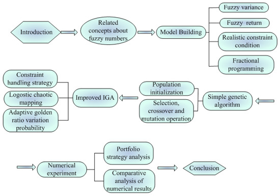
Figure 1.
Full text frame diagram.
2. Preliminaries
Fuzzy set theory was first proposed by Zadeh [6], which is mainly used to describe the fuzzy uncertainty of information. Fuzzy number is actually a special form of fuzzy set. Fuzzy number and its related concepts are briefly introduced below.
Definition 1
([27]). Assuming is a mapping of X to the range , where , say is fuzzy set on the X, and the function is the membership function of fuzzy set , called x for fuzzy sets membership degree.
Definition 2
([27]). Fuzzy set has membership function ; to call it fuzzy number , it must meet the following conditions:
- (1)
- is regular, exist make ;
- (2)
- is convex, means when , have , and also have ;
- (3)
- is upper semi-continuous and bounded, which means , grep is a fuzzy support set;
- (4)
- is a compact set, which also is a support set of .
Definition 3
([9]). A fuzzy number , is a trapezoid fuzzy number for interval [a,b], α is the fuzzy number left width, β is the right width of the fuzzy number. The fuzzy number can be derived from this In γ− level cut sets the following probability mean and variance are:
Assuming is a trapezoidal fuzzy number, then its membership function [28] can be expressed as:
The − level cut of the trapezoidal fuzzy number is: , of which , , . is called the confidence level or confidence level, and , respectively, are − the left and right endpoints of the horizontal cut set.
Therefore, based on Definition 3, the possibility mean and possibility variance of the trapezoidal fuzzy number are expressed as follows:
Theorem 1
([29]). Assuming the  is any given n fuzzy numbers, and is a real number, then
where is a symbolic function.
is any given n fuzzy numbers, and is a real number, then
where is a symbolic function.
is any given n fuzzy numbers, and is a real number, then3. Fuzzy Multi-Period Portfolio Model
This section is divided into two parts. The first part is the explanation of the related symbols used in this paper. The second part is the process of establishing a fuzzy multi-period portfolio model considering various practical constraints.
3.1. Related Symbol Specification
Suppose investors distribute their wealth among n securities with uncertain returns to obtain the final wealth for period T. Assume that the rates of return of different periods are independent of each other, and the rate of return is represented as a trapezoidal fuzzy variable. For convenience, we present the economic implications of the symbols used in this article in Table 2.
Table 2.
The symbols used in the modeling.
3.2. Fractional Programming Multi-Period Portfolio Model with Realistic Constraints in Fuzzy Environment
As mentioned earlier, incorporating constraints such as cardinality constraints into the portfolio selection model will result in more realistic and reasonable portfolios. In this paper, we consider several practical constraints to improve the portfolio selection model.
- Cardinality constraint
The number of investments in a large number of securities cannot exceed a predefined upper limit, and this number is referred to as the cardinality. If asset i is held in period t, ; otherwise, . The specific situation can be represented as follows:
Assuming that the maximum limit for the number of assets in a portfolio in period t is K, the cardinality constraint is expressed as follows:
- Asset holding limits
To ensure that the investment allocation for each security is within a specific range, with a given minimum and maximum , such that , considering the cardinality constraint mentioned above, the representation of investment portfolio asset holding with cardinality constraint can be obtained as follows:
- Limit on the proportion of total investment
In the investment process, it is generally assumed that the sum of the investment proportion of assets is 1, that is
- Terminal wealth
As defined in Definition 3, the fuzzy possibility mean of the portfolio return in period t can be represented as follows:
In the real stock exchange market, transaction cost has a great impact on investment return, which will directly affect the final return of the investment portfolio. Similar to the study in the literature [29], this paper adopts the V-shaped transaction cost function. That is, the transaction cost of securities i in period t can be expressed as:
where represents the transaction cost rate in period t, is the investment portfolio in period t − 1, and is the current investment portfolio in period t. Therefore, the total investment cost of Phase t is
Taking into account the transaction costs, the fuzzy possibility mean of the net return of the portfolio in period t, after deducting the transaction costs, can be calculated as follows:
Furthermore, there exists the following relationship between the fuzzy expected value of the end-of-period t wealth and the fuzzy expected value of the end-of-period t − 1 wealth:
By repeatedly iterating the above equation, we can obtain the expected values of the terminal wealth, , and cumulative wealth, , over the entire investment period, represented as follows:
- Fuzzy risk
According to Definition 3, the possibility variance, , of the investment portfolio in period t can be represented as:
Furthermore, according to Definition 3 and Theorem 1, the final risk obtained by multiplying the risks of each period of the investment portfolio over the entire investment period is:
Similarly, using Definition 3 and Theorem 1, we can also derive the cumulative risk of the investment portfolio over the entire investment period [26] as:
In the securities market, investors usually want to reduce risk while increasing the return on their investment portfolios. However, maintaining this perfect equilibrium is frequently difficult in practice, and concessions must be made. In this study, we develop an investment portfolio model with the goal function of minimizing the product of risk and return ratios over various periods. This seeks to establish as much balance as possible between the two objectives. The return on the portfolio in period t is determined based on the performance in period t − 1, allowing investment outcomes to be transmitted over many periods. Based on this, and assuming that the expected return is more than and the risk is less than , we develop the fractional programming multi-period investment portfolio model MMFVCCPO, which has realistic constraints in a fuzzy environment and can be represented as:
The MMFVCCPO model’s goal function is to minimize the product of the risk–return ratios of each period throughout the whole investment term. The aim is to reduce the product of each period’s risk–return ratios while assuring the lowest risk–return ratio in each period. The model’s first constraint stipulates that the investment portfolio’s return in period t must be greater than or equal to the specified . The second constraint indicates that the expected value of the wealth method at the beginning of the t period is calculated memorically on the basis of the previous period, reflecting the continuity of multi-period investment. The third restriction specifies that the investment portfolio’s risk in period t cannot exceed . The fourth restriction reflects the amount of assets in the investment portfolio in period t, which must be fewer than or equal to K. The fifth constraint, which is a binary vector with values of 0 or 1, represents the holding status of an asset in the investment portfolio. The sixth constraint reflects a restriction on the investment percentage in asset i, which requires the investment proportion in asset i to be between . The seventh criterion is the aggregate of investment proportions, which must be greater than one.
It should be observed that each of the preceding constraints has T smaller constraints, each of which corresponds to T periods. The following are the benefits of adding fractional programming: (1) It reduces the complexity of the problem by converting the original multi-objective problem to a single-objective problem. (2) When comparing risk and return, it attempts to minimize risk while maximizing return, treating both objectives equally. It is not necessary to give up the weight of one goal in order to achieve the other, i.e., there is no priority differential. It can, to some extent, strike an ideal balance between the two goals.
4. Solution Method for Model
This section is divided into two parts. The first part introduces the method of constraint processing in the model. The second part is an improved genetic algorithm for the model.
4.1. Constraint Processing Method (Semi-Penalty Function Method)
The semi-penalized function approach solves nonlinear constrained optimization problems numerically. It converts complicated restrictions into penalty terms in the objective function, resulting in a sequence of optimization problems with smaller constraints.This approach is used in this study to address the first three constraints in the MMFVCCPO model. In the model, the penalty terms for the equality and inequality requirements are defined as follows:
Based on the equation above, the penalty function for the MMFVCCPO model is defined as follows:
where represents the objective function value and L represents the penalty factors applied to the equality and inequality constraints. Thus, the MMFVCCPO model can be formulated as the constrained optimization problem SPFM as follows:
The investment portfolio model is turned into a sequence of restricted optimization problems to solve the penalty coefficients using the semi-penalized function approach described above. Furthermore, in the methodology part, this study develops an approach for dealing with cardinality restrictions and uses normalization methods to deal with additional constraints individually. For further information, please see Section 4.2. Using the semi-penalty function method to deal with constraints can ensure that, when an infeasible solution occurs, a penalty is imposed to ensure that the solution is in the feasible region. Secondly, the cardinality constraint processing strategy and normalization method also ensure that the solution is in the feasible domain before proceeding to the next step, so the IGA designed in this paper can ensure that the global optimal solution is obtained.
The SPFM model remains a nonlinear mixed-integer fractional programming problem after being processed using the semi-penalized function approach, which is challenging to solve using typical optimization methods. To solve the SPFM model, we offer an enhanced genetic algorithm dubbed IGA, which incorporates the semi-penalized function technique. In this part, we will first study the traditional genetic algorithm before introducing modifications such as the penalty function technique.
4.2. The Proposed Improved Genetic Algorithm, IGA
This part mainly includes the basic genetic algorithm, improved genetic algorithm, and convergence proof of improved algorithm.
4.2.1. Basic Genetic Algorithm
The genetic algorithm (GA) is a random search optimization approach based on natural selection and population genetic mechanisms. It was developed by Professor J. H. Holland [30] of the University of Michigan and is now widely utilized in optimization issues in a variety of engineering domains. It simulates the replication, crossover, and variation phenomena that occur in natural selection and heredity and applies the concept of survival of the fittest by Michalewicz [31] to start from any initial population and efficiently searching for a coded parameter space through the randomization technology of selection, crossover, and mutation operations to generate a group of individuals more suitable for the environment, which ensures the population evolves to better and better regions in the search space, so that generation after generation continues to reproduce and evolve, eventually converges on a group of individuals that are most adapted to the environment, resulting in a high-quality solution to the issue. As a result, genetic algorithms may be viewed as a process of continual development of a population of viable solutions. It is worth mentioning that the five key elements of a genetic algorithm are parameter coding, starting population setup, fitness function design, genetic operation design, and control parameter setting. The following are the primary characteristics of the genetic algorithm (Algorithm 1): (1) It directly act on the structural object, with no qualification for derivation or function continuity. (2) Using the probabilistic optimization approach, the optimum search space may be generated and directed automatically without the need for specific rules, and the search direction can be altered adaptively.
- (1)
- Select Operator: The procedure of picking excellent people from a group and weeding out bad people is referred to as a selection operation. To ensure that the next generation is a good individual, select individuals using the roulette method to the greatest extent individual, i, for the selected probability , where is individual fitness value and is the sum of all individual fitness values in the population.
- (2)
- Crossover operator: Cross operation refers to the operation of replacing and recombining part of the structure of two parent individuals to produce a new individual; the purpose of cross is to produce a new individual in the next generation. Randomly selected from two individuals, to exchange, to the parent genes passed on to the next generation, to produce a new individual. Chromosome and chromosome on j make a cross as follows:where b is a random number in the range .
- (3)
- Mutation operator: Mutation manipulation occurs when the gene values on some locus in the coding string of an individual chromosome are replaced with the remaining alleles on that locus to form a new individual. The mutation operation of the first j gene, , of the first individual, i, is:where is ceiling, is floor, , for the random number, g for the current number of iterations, for the maximum number of iterations, r to random number.
| Algorithm 1 Pseudo−Code of the Standard Genetic Algorithm |
| Input: Set initialization parameters; |
Output: Optimum solution;
|
4.2.2. The Proposed Improved Genetic Algorithm, IGA
In the literature [32,33,34], the theoretical concept of the genetic algorithm is elaborated in detail, and the latest progress of the genetic algorithm in recent years is analyzed, summarized, and prospected. Based on this, it can be seen that, for the heuristic algorithm, it is very important to find a balance between exploration and exploitation. Exploration refers to the movement of discovering completely new areas in the search space, while exploitation refers to the movement of focusing the search in the vicinity of promising known solutions during the search. Based on the above discussion, an improved IGA is proposed to solve the SPFM model, which has both 0–1 and general integral constraints. In particular, we use logistic chaos mapping to generate chaotic initial sequences and an improved golden ratio variation probability formula to control individual randomization motion. Using this strategy, the balance of exploration and development ability is further improved, and good results are obtained.The improved IGA algorithm provides portfolio strategies under different constraints that satisfy the clear constraints imposed by investors. The flow chart of the improved algorithm is shown in Figure 2.
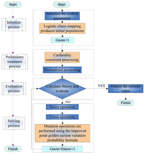
Figure 2.
Flow chart of the improved IGA algorithm.
- (1)
- Population initialization
A D-dimensional vector is randomly generated using decimal real coding, with each chromosome as a real vector. Then, a non-periodic, non-convergent chaotic sequence sensitive to initial values is generated using logistic mapping. The logistic mapping formula is as follows:
where is the mapping parameter and is the random number of . The use of a chaotic sequence to generate the initial population makes the initial solution more evenly distributed in the solution space, which helps to enhance the diversity of the population, jump out of the local optimal, achieve global balance, and obtain better results than the pseudo-random number calculation.
- (2)
- Cardinality constraint process
Here, we propose a cardinal constraint processing strategy for the cardinal constraint , so that the cardinal constraint can be handled more reasonably and effectively and play a more significant role in simulating investment. In addition, the model can meet the needs of different investors for the investment base by changing the maximum limit of the base in the simulation process, so as to increase the applicability of the model and take into account the impact of realistic factors to achieve the purpose of maximum investment return and minimum risk. The method is divided into the following two steps:
- (a)
- Calculation is not zero in each individual chromosome number P, where , K for a given the biggest asset investment base;
- (b)
- Determine whether the value of P satisfies the inequality constraint . If the inequality is satisfied, proceed to the next step. Otherwise, randomly select at the corresponding position of p of and set it to 0, so that the value of P satisfies the inequality constraint , and the specific pseudo-code is Algorithm 2.
| Algorithm 2 Cardinality Constraint Handling Strategy |
| Input: Initial |
| Output: Initial population X |
|
- (3)
- Adaptive golden section mutation operator
In order to reduce the probability of a mutation in a good individual gene causing a significant decline in fitness when the number of iterations is high, an adaptive mutation operator is proposed. The specific feature is that in order to expand the search scope of the optimal path and improve the mutation probability when the number of algorithm iterations is relatively small, the mutation probability gradually decreases with the increase of the number of iterations, so as to prevent the good individuals from introducing bad genes due to mutations in the later period. Since the variation performance of a single variable fitted with an exponential function is more suitable for the evolution process of a population, the golden section variation probability formula designed in this paper is as follows:
where is the mutation probability, is the maximum value of the mutation probability, is the preset maximum number of iterations, is the current number of iterations, and . In this paper, the idea of the golden section is introduced, and is set as 0.618, corresponding to , which can make the variation probability change in the golden ratio trend to a certain extent and increase the population diversity. In addition, to a certain extent, it can avoid the situation that the algorithm cannot converge as soon as possible because the mutation probability is too large. Based on the mutation probability obtained by the above formula, a random method is adopted to select individuals from the population for mutation operation to produce a new generation of individuals.
- (4)
- Evaluation function
The fitness function is also called the evaluation function, which refers to the degree of superiority of an individual in the survival of a population. It is mainly used to judge the fitness of individuals through individual characteristics, which is used to distinguish the “good and bad” of individuals. The degree of infeasible solutions depends not only on the number of constraints violated but also on the number of solutions at hand. However, the degree of a feasible solution is always mixed, equal to its objective function value. Therefore, according to the penalty function method discussed in Section 4.1, the fitness function, , of the SPFM model can be expressed as:
the initial value of the penalty factor , and the iterative formula is . The pseudo-code of the improved algorithm is shown in (Algorithm 3).
| Algorithm 3 Pseudo-Code of the Improved IGA |
| Input: Set initialization parameters; |
| Output: Optimum solution |
|
- (5)
- Complexity analysis of IGA
Time complexity reflects the execution efficiency of an algorithm and refers to the relationship between the execution time and the input value. Let be the time complexity of IGA. can be obtained by the formula:
where M is the maximum number of iterations of the algorithm and N is the population size.
4.2.3. Proof of Convergence for IGA
In this section, we prove the convergence of the improved genetic algorithm by building a series convergence model. For a global optimization problem, the optimal solution is first assumed to be , then the optimal value is . The optimal solution of the improved genetic algorithm in the t iteration is , and accordingly is the current optimal value. According to the convergence theorem of series, the equivalent condition of the improved genetic algorithm to find the global optimal value is that some is in the neighborhood of the optimal value . For any , was established.
In the iterative process of improving the genetic algorithm, each iteration will obtain an optimal individual. We define the set of these individuals as follows:
In the above formula, is the maximum number of iterations. Obviously, the sequence can be constructed according to the above formula as follows:
According to the update strategy selected by the optimal individual, in the improved genetic algorithm the individual change strategy can ensure that the optimal value of each generation must not be inferior to the previous generation, that is, . It can be seen that the following formula is valid:
With the continuous evolution of the population, individuals in the population will continue to move closer to the range of the optimal solution; that is, the probability that the optimal value searched by the current population will enter the neighborhood of the global optimal value gradually increases. The optimal values of the current population, , converge to the global optimal value, , probability and are defined as follows:
According to the above two formulas, the following relationship can be obtained:
Therefore, the probability that the current optimal value does not converge to the global optimal value after the t iteration is:
From the above formula, we can see that is monotonically decreasing, so the following formula is valid:
where is probability, meet , in which . After t iterations, the following formula can be obtained:
As can be seen from the above formula, after several iterations the probability that the improved genetic algorithm does not converge to the optimal value is 0. Therefore, as the number of iterations increases, the improved genetic algorithm will eventually converge to the global optimal solution, , with probability 1, q.e.d.
5. Numerical Example
In this study, we improved the genetic algorithm to better solve the SPFM problem. In order to explain the idea of our model and the algorithm designed, this paper selects all the sample stocks in the SSE 50 as the research object. However, since the 50 sample stocks of the SSE 50 are adjusted every six months, the fund will adjust its position, so the transferred stocks have a certain negative and the transferred stocks have a certain positive. The 50 stocks of SSE 50 are dynamically adjusted. Considering the concept that the sample stocks should have strong stability, and in order to ensure that the research results are more valuable for reference, it is necessary to screen the 50 stocks of SSE 50 to remove the stocks with obvious problems, fewer selections, serious lack of year data, and inconsistent data. The stocks in the previous dynamic adjustment list of the Shanghai Stock Exchange 50 were retained rather than fixed (no obvious problems, always selected, complete and consistent data, and easy to obtain), and finally 30 alternative sample stocks with stable performance were obtained. All trading-day data of these stocks from 1 January 2017 to 1 January 2020 are selected as the raw data for empirical analysis. This paper takes one year as an investment cycle when simulating investment, which is divided into three cycles altogether. These data are from https://tr.investing.com/ accessed on 3 September 2023. The selected sample covers a number of industries with different income characteristics, which satisfies decentralization and can effectively reduce non-systemic risks in investment. Therefore, a choice more in line with investors’ wishes can increase the significance of empirical research on stock portfolio models. All experiments in this paper were carried out on MATLAB 2016a, and the computer processor was an Intel(R) Core(TM) i7-10700 CPU @ 2.90 GHz 2.90GHz, Windows 10.
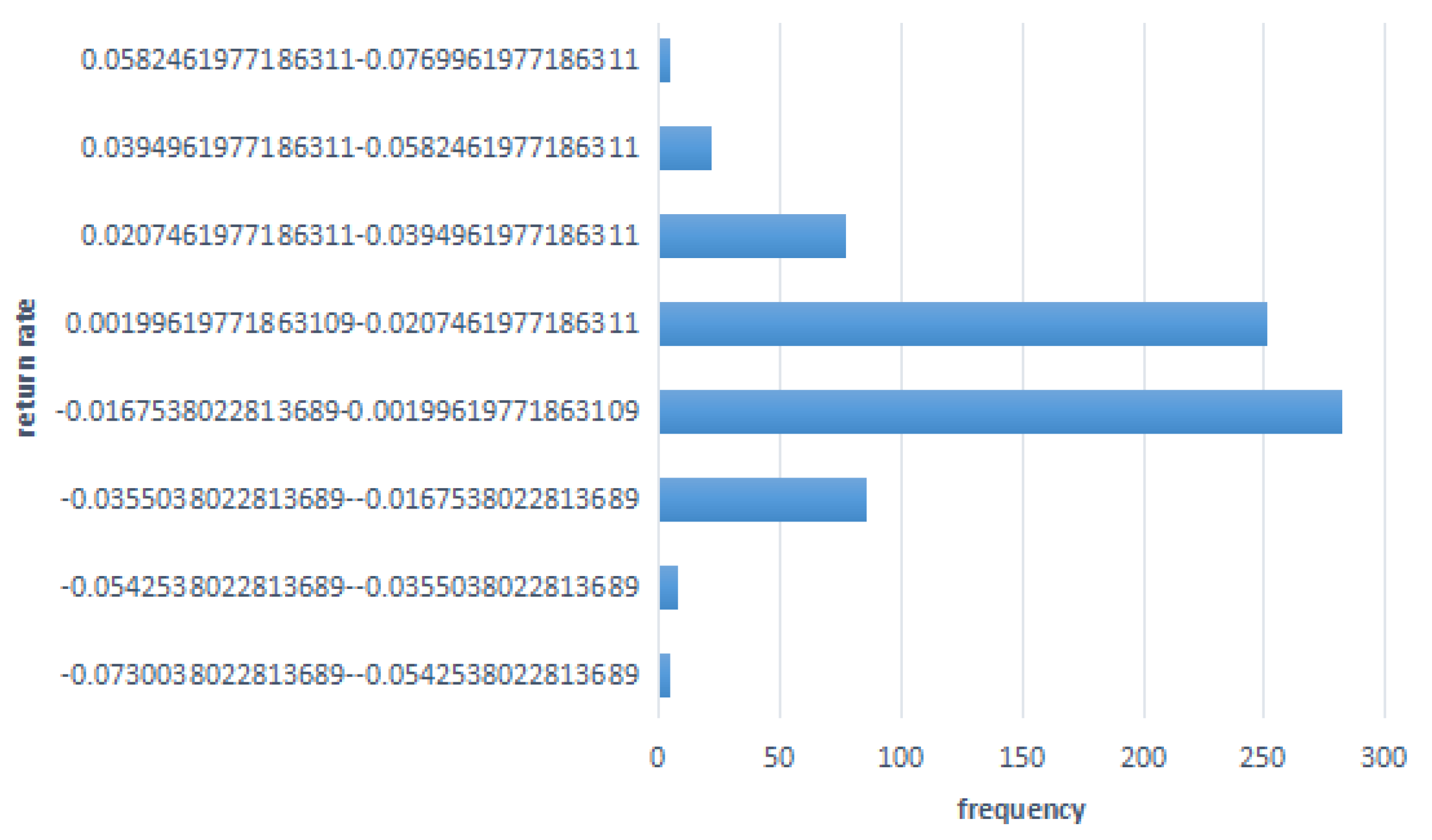
In portfolio theory, the use of trapezoidal fuzzy numbers and triangular fuzzy numbers can help investors better deal with uncertainty and ambiguity, so as to carry out more effective asset allocation and risk management. Trapezoidal fuzzy numbers are suitable for more complex and diverse portfolio modeling and risk management, while triangular fuzzy numbers are suitable for relatively simple and intuitive portfolio description and analysis. In view of the complexity of the theory and research problem, this paper chooses to use ladder fuzzy numbers to quantify the return rate of the investment portfolio. The trapezoidal fuzzy number for estimating the rate of return is approximated using the method of objective fuzzy frequency statistics. Taking 600031 as an example, the specific method is as follows: Calculate the daily rate of return of the stock for the past three years and provide the frequency distribution graph of the rate of return, as shown in Figure 3. From the graph, it can be seen that the rate of return is mainly concentrated between (−0.0168, 0.0020) and (0.0020, 0.0207). First, calculate the mean of the historical rate of return between (−0.0168, 0.0020) as −0.0076 and take it as the left endpoint of the tolerance interval. Then, calculate the mean of the historical rate of return between (0.0020, 0.0207) as 0.0094 and take it as the right endpoint of the tolerance interval. Sort the historical rate of return in ascending order, select the rate of return −0.0346 on the third trading day in the interval (−0.0355, −0.0168) as the minimum possible value, and take the rate of return 0.0211 on the second trading day in the interval (0.0207, 0.0395) as the maximum possible value. Thus, the left width is 0.0563 and the right width is 0.0562. Finally, the trapezoidal fuzzy number for 600031 is (−0.0076, 0.0094, 0.0563, 0.0562). For ease of calculation, the minimum possible value, left endpoint, right endpoint, and maximum possible value of the trapezoidal fuzzy number are taken as the four parameter values of the fixed possibility distribution of the trapezoidal fuzzy variable for 600031, which is (−0.0346, −0.0076, 0.0094, 0.0211). According to this method, the fuzzy rate of return distribution for the sample stock is shown in next. It should be noted that, in this case, the trapezoidal fuzzy number for estimating the rate of return is approximated.
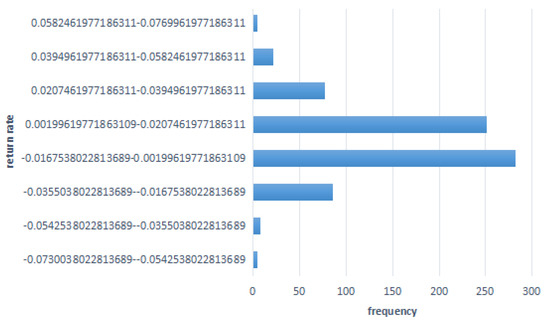
Figure 3.
Frequency distribution histogram.
The other parameters associated with the proposed model are shown in Table 3. For the uncertainty distribution of the thirty securities, , see Table 4. In addition, assume that the desired number of securities in the portfolio .
Table 3.
The parameter settings for comparison of the algorithm.
Table 4.
Fuzzy yield distribution of 30 sample stocks.
The experimental part mainly includes the following five parts:
- (1)
- Analyze portfolio strategies under different base constraints to reflect the impact of cardinality constraints on the portfolio;
- (2)
- Analyze the portfolio strategy under the previous and next limits of different investment ratios in order to analyze the influence of different parameters of the upper and lower limits of investment ratios on the portfolio;
- (3)
- The numerical results of solving the SPFM model by different algorithms are compared to verify the effectiveness of the IGA proposed in the next paper;
- (4)
- Verify the influence of the adjustment for cost rate parameters on the numerical results by comparing the numerical results under different algorithms and different transaction cost rates;
- (5)
- The numerical results of different algorithms under different iterations were analyzed for comparative analysis to highlight the impact of iterations on numerical results, and the numerical results of other comparison algorithms were also compared.
5.1. Experimental Results
In this section, we run each test 10 times and find the average. We adopted the proposed IGA algorithm to solve the SPFM model. In order to show the influence of cardinality constraints on portfolio selection, the calculation results for different K are given in Table 5 and Table 6. Obviously, as K changes, so does the optimal portfolio. In fact, the greater the K, the greater the return and risk of the portfolio.
Table 5.
Optimal investment strategies under different values of K.
Table 6.
Optimal investment strategies under different values of K.
Table 5 and Table 6 exhibit the calculation results for various cardinalities to demonstrate the influence of cardinality constraints on portfolio selection. The SPFM model’s portfolio strategy is shown in Table 5 and Table 6 when the cardinality constraint is , , , , and . According to the table, the model has distinct weight allocation modifications for the investment share of each asset in each phase. Obviously, the ideal portfolio changes as cardinality K changes. In fact, the broader the cardinality, the greater the portfolio’s return and risk. From the table, it can be seen that the investment frequency for assets 17, 22, 24, and 30 is relatively high under different base restrictions and time periods. The investment weight for assets 11, 3, 20, 23, 24, and 17 is also relatively high, indicating that investors have a strong positive outlook on these assets and that investing in them can bring greater returns to investors. Additionally, it can be observed that the returns and risks of the investment portfolio increase with longer investment periods. We also conducted a similar analysis of portfolio results under different upper and lower bound constraints of asset holdings, as detailed in Table 7, Table 8, Table 9 and Table 10.
Table 7.
Optimal investment strategies under different upper bounds .
Table 8.
Optimal investment strategies under different upper bounds .
Table 9.
Optimal investment strategies under different lower bounds .
Table 10.
Optimal investment strategies under different lower bounds .
If , then and . Then, Table 7 and Table 9 present optimum portfolio methods for various boundary restrictions. Table 7 lower bounds are , whereas Table 9 upper bounds are . Table 7 and Table 9 show that the investment portfolio strategy changes when the upper and lower boundaries shift. According to the tables, the SPFM model modifies the distribution of investment weights for each asset in each period. It is obvious that the optimal investment portfolio varies when the boundary restrictions change. The tables show that there is a greater investment frequency for assets 13, 21, and 28 under varied lower bound constraints and periods. Furthermore, assets 4, 7, 13, 22, 23, 28, 29, and 30 have a larger investment weight. Similarly, for different upper bound constraints and durations, assets 7, 13, 21, and 28 have a greater investment frequency, while assets 2, 7, 11, 13, 21, and 28 have a larger investment weight. This suggests that investors are optimistic about these assets and believe that investing in them will provide higher returns. Furthermore, the investment portfolio’s rewards and hazards rise as the investment time lengthens.
Table 8 and Table 10 provide numerical findings such as mean, standard deviation, and calculation time for various boundary restrictions. The findings clearly varied depending on the upper and lower boundaries used. Notably, when the upper and lower limits are set to 0.5 and 0.005, respectively, the computation time is the shortest. Furthermore, through the comparison of standard deviation values, it can be seen that the fluctuation of numerical results in this case is relatively stable. This implies that adopting upper and lower limits of 0.5 and 0.005 is also reasonable and feasible in other computing processes, and better results will be obtained.
5.2. Performances of the Proposed IGA
To evaluate the performance of the IGA algorithm, we compared it to the standard DE, GA, I-GA, and GGA. In the following experiments, the values of the control parameters used for comparison are shown in Table 3. In addition, for the proposed SPFM model we assume that = 10,000, , .
Different algorithms were used to analyze the mean value and standard deviation (SD) of the optimal target and other performance indicator parameters. Table 11, Table 12 and Table 13 lists the average results of 10 independent runs under different cardinal numbers, different transaction costs, and different iterations.
Table 11.
Performance comparisons under different values of K.
Table 12.
Performance comparisons under different rates of transaction costs rate.
Table 13.
Performance comparisons under different iterations.
Table 11 shows the comparison of numerical results of different algorithms under different base restrictions. It can be seen that, in the change process from cardinals k = 5 to k = 25, the number of times IGA numerical results are better than the other algorithms are 3,5,4,5,4, respectively. I-GA is 1,1,1,2,1; GGA is 1,1,0,0,1; GA is 2,0,2,0,1; DE is 1,1,1,1,1. Table 12 shows the comparison of the numerical results of different algorithms under different transaction costs. It can be seen that in the process of the change of transaction costs, c = 0, c = 0.003, and c = 0.005, the number of times that IGA numerical results are better than the other algorithms are 6,6,2, respectively. I-GA is 0,0,1; GGA is 0,0,2; GA is 1,1,2; DE is 1,1,1. Table 13 shows the comparison of the numerical results of the different algorithms under different iterations. It can be seen that during the change of iterations 100, 200, and 300, respectively, the number of times IGA numerical results are better than the other algorithms is 5,5,4, respectively. I-GA is 0,0,0; GGA is 1,1,2; GA is 0,1,0; DE is 2,1,2. It is obvious that IGA obtains the optimal value more times than other algorithms in Table 11, Table 12 and Table 13. On the whole, the average value, standard deviation, terminal wealth, cumulative risk, and other numerical results obtained by the IGA proposed in this paper are better than those listed by the other algorithms. At the same time, the time required for IGA computation is also less than the other algorithms in most cases. In other words, the proposed IGA is more accurate than some other standard heuristic algorithms. In addition, we can also see that when the SD value of the IGA is lower, it indicates that the algorithm in this paper cannot only obtain more high-quality solutions but is also more stable and reliable in finding high-quality solutions.
Table 14 is a summary analysis of the numerical results in Table 11, Table 12 and Table 13. It can be seen from Table 14 that the probability of the numerical results of IGA proposed by us reaching the optimal value under different parameters is 52.5%, 58.33%, and 58.33%, respectively, which is much higher than the probability of obtaining the optimal value times of the other algorithms. Specifically, it can be seen that the probability of the IGA obtaining the optimal value under different performance indicators is at least 37.5% higher than the other algorithms. It can be concluded that the IGA in this paper is superior to the other algorithms in terms of computational performance.
Table 14.
The comparison of the optimal probabilities of different algorithms under different parameters.
In summary, the obtained results clearly show that the IGA method has superior performance in terms of convergence, speed, stability, and robustness compared with the other algorithms. Therefore, the IGA method can be considered as a good choice for dealing with complex portfolio optimization problems.
6. Conclusions
Aimed at the complexity of the financial market, this paper establishes a fractional programming multi-period portfolio model under the fuzzy framework, considering multiple realistic constraints, and designs an improved genetic algorithm to solve the model. The established approach examines risk and return at the same level, without prioritization, and eliminates the flaw in which the generic multi-objective model must sacrifice one aim to achieve another while solving. Moreover, the probability of the IGA obtaining the optimal value under different performance indexes is at least 37.5% higher than other algorithms. However, when addressing a limited optimization issue with three or more objective functions, the fractional technique is more difficult than the multi-objective method, which does not have to deal with contradicting relationships between the goals. Second, because investors make the majority of decisions, adding investing behavior and psychology into portfolio modeling yields a more realistic and practical model. In the next modeling, we will also explore combining these two elements into the model to create a more comprehensive portfolio model. At the same time, the fractional programming proposed in this study may be applied not only to two-objective issues but also to multi-objective optimization problems. In this regard, we shall carry out additional study. Equally important, we will focus our future research on optimizing the design of multi-objective algorithms to tackle this type of issue directly while minimizing conflict.
Author Contributions
Conceptualization, C.H.; methodology, C.H.; software, C.H.; validation, C.H.; formal analysis, C.H.; investigation, E.G.; resources, C.H.; data curation, C.H.; writing—original draft preparation, C.H.; writing—review and editing, C.H.; visualization, preparation, C.H.; writing—review and editing, C.H.; visualization, C.H.; supervision, E.G., C.H., and Y.G.; project administration, Y.G.; funding acquisition, Y.G. and C.H. All authors have read and agreed to the published version of the manuscript.
Funding
This research was supported in part by the Natural Science Foundation Key Projects of Ningxia, grant number 2022AAC02043, in part by the Construction Project of First-class Subjects in Ningxia Higher Education, grant number NXYLXK2017B09, in part by the Major Special Fund of North Minzu University, grant number ZDZX201901, in part by the Nanjing Securities Support Basic Discipline Research Project, grant number NJZQJCXK202201, and in part by the Major Proprietary Funded Project of North Minzu University, grant number YCX23224.
Data Availability Statement
The data are free to download from the website https://tr.investing.com/, accessed on 3 September 2023.
Conflicts of Interest
The authors declared no conflicts of interest.
References
- Markowitz, H.M. Portfolio selection. J. Financ. 1952, 7, 77. [Google Scholar]
- Plachel, L. A unified model for regularized and robust portfolio optimization. Econ. Dyn. Control 2019, 109, 103779. [Google Scholar] [CrossRef]
- Wang, W.; Li, W.; Zhang, N.; Liu, K. Portfolio formation with preselection using deep learning from long-term financial data. Expert Syst. Appl. 2020, 143, 113042. [Google Scholar] [CrossRef]
- Chen, W.; Zhang, H.; Mehlawat, M.K.; Jia, L. Mean–variance portfolio optimization using machine learning-based stock price prediction. Appl. Soft Comput. 2021, 100, 106943. [Google Scholar] [CrossRef]
- Ma, Y.; Han, R.; Wang, W. Portfolio optimization with return prediction using deep learning and machine learning. Expert Syst. Appl. 2021, 165, 113973. [Google Scholar] [CrossRef]
- Zadel, L.A. Fuzzy sets. Inf. Control 1965, 8, 338–353. [Google Scholar]
- Katagiri, I. Chance constrained bottleneck spanning tree problem with fuzzy random edge costs. J. Oper. Res. Soc. Jpn. 2000, 43, 128–137. [Google Scholar] [CrossRef]
- Pahade, J.K.; Jha, M. A Hybrid Fuzzy-SCOOT Algorithm to Optimize Possibilistic Mean Semi-absolute Deviation Model for Optimal Portfolio Selection. Int. J. Fuzzy Syst. 2022, 24, 1958–1973. [Google Scholar] [CrossRef]
- Pahade, J.K.; Jha, M. Credibilistic variance and skewness of trapezoidal fuzzy variable and mean–variance–skewness model for portfolio selection. Results Appl. Math. 2021, 11, 100159. [Google Scholar] [CrossRef]
- Gupta, P.; Mehlawat, M.K.; Khan, A.Z. Multi-period portfolio optimization using coherent fuzzy numbers in a credibilistic environment. Expert Syst. Appl. 2021, 167, 114135. [Google Scholar] [CrossRef]
- Mehlawat, M.K.; Gupta, P.; Khan, A.Z. Multiobjective portfolio optimization using coherent fuzzy numbers in a credibilistic environment. Int. J. Intell. Syst. 2021, 36, 1560–1594. [Google Scholar] [CrossRef]
- Gao, W.; Sheng, H.; Wang, J.; Wang, S. Artificial bee colony algorithm based on novel mechanism for fuzzy portfolio selection. IEEE Trans. Fuzzy Syst. 2018, 27, 966–978. [Google Scholar] [CrossRef]
- Vercher, E.; Bermúdez, J.D. Portfolio optimization using a credibility mean-absolute semi-deviation model. Expert Syst. Appl. 2015, 42, 7121–7131. [Google Scholar] [CrossRef]
- Leung, M.-F.; Wang, J.; Che, H. Cardinality-constrained portfolio selection via two-timescale duplex neurodynamic optimization. Neural Netw. 2022, 153, 399–410. [Google Scholar] [CrossRef] [PubMed]
- Leung, M.-F.; Wang, J. Cardinality-constrained portfolio selection based on collaborative neurodynamic optimization. Neural Netw. 2022, 145, 68–79. [Google Scholar] [CrossRef] [PubMed]
- Meng, X.; Zhou, X. Multi-period Fuzzy Portfolio Selection Model with Cardinality constraints. In Proceedings of the 2019 16th International Conference on Service Systems and Service Management (ICSSSM), Shenzhen, China, 13–15 July 2019. [Google Scholar]
- Zhao, H.; Chen, Z.G.; Zhan, Z.H.; Kwong, S.; Zhang, J. Multiple populations co-evolutionary particle swarm optimization for multi-objective cardinality constrained portfolio optimization problem. Neurocomputing 2021, 430, 58–70. [Google Scholar] [CrossRef]
- Yang, M.; Qian, W.; Yang, L.; Hou, X.; Yuan, X.; Dong, Z. A Synergistic Multi-Objective Evolutionary Algorithm with Diffusion Population Generation for Portfolio Problems. Mathematics 2024, 12, 1368. [Google Scholar] [CrossRef]
- Delikta, D.; Ustun, O. Multi-objective genetic algorithm based on the fuzzy MULTIMOORA method for solving the cardinality constrained portfolio optimization. Appl. Intell. 2022, 53, 14717–14743. [Google Scholar] [CrossRef]
- Alshraideh, M.A.; Mahafzah, B.A.; Salman, H.S.E.; Salah, I. Using genetic algorithm as test data generator for stored PL/SQL program units. J. Softw. Eng. Appl. 2013, 6, 65–73. [Google Scholar] [CrossRef]
- Chen, W.; Li, D.; Liu, Y.J. A novel hybrid ICA-FA algorithm for multiperiod uncertain portfolio optimization model based on multiple criteria. IEEE Trans. Fuzzy Syst. 2018, 27, 1023–1036. [Google Scholar] [CrossRef]
- Liu, Y.J.; Zhang, W.G.; Gupta, P. Multiperiod portfolio performance evaluation model based on possibility theory. IEEE Trans. Fuzzy Syst. 2019, 28, 3391–3405. [Google Scholar] [CrossRef]
- Yang, X.Y.; Chen, S.D.; Liu, W.L.; Zhang, Y. A Multi-period fuzzy portfolio optimization model with short selling constraints. Int. J. Fuzzy Syst. 2022, 24, 2798–2812. [Google Scholar] [CrossRef]
- Li, X.; Qin, Z. Interval portfolio selection models within the framework of uncertainty theory. Econ. Model. 2014, 41, 338–344. [Google Scholar] [CrossRef]
- Zhang, B.; Peng, J.; Li, S. Uncertain programming models for portfolio selection with uncertain returns. Int. J. Syst. Sci. 2015, 46, 2510–2519. [Google Scholar] [CrossRef]
- Qin, Z.; Kar, S.; Zheng, H. Uncertain portfolio adjusting model using semiabsolute deviation. Soft Comput. 2016, 20, 717–725. [Google Scholar] [CrossRef]
- Chen, W.; Wang, Y.; Gupta, P.; Mehlawat, M.K. A novel hybrid heuristic algorithm for a new uncertain mean-variance-skewness portfolio selection model with real constraints. Appl. Intell. 2018, 48, 2996–3018. [Google Scholar] [CrossRef]
- Zhang, W.G.; Wang, Y.L. Notes on possibilistic variances of fuzzy numbers. Appl. Math. Lett. 2007, 20, 1167–1173. [Google Scholar] [CrossRef]
- Deb, K. An efficient constraint handling method for genetic algorithms. Comput. Methods Appl. Mech. Eng. 2000, 186, 311–338. [Google Scholar] [CrossRef]
- Holl, J.H. Genetic algorithms. Sci. Am. 1992, 267, 66–73. [Google Scholar]
- Michalewicz, Z. Genetic Algorithms + Data Structures = Evolution Programs; Springer: Berlin/Heidelberg, Germany, 1999. [Google Scholar]
- Katoch, S.; Chauhan, S.S.; Kumar, V. A review on genetic algorithm: Past, present, and future. Multimed. Tools Appl. 2021, 80, 8091–8126. [Google Scholar] [CrossRef]
- Lambora, A.; Gupta, K.; Chopra, K. Genetic algorithm-A literature review. In Proceedings of the 2019 IEEE International Conference on Machine Learning, Big Data, Cloud and Parallel Computing (COMITCon), Faridabad, India, 14–16 February 2019; pp. 380–384. [Google Scholar]
- Liu, Y.-J.; Zhang, W.-G. A multi-period fuzzy portfolio optimization model with minimum transaction lots. Eur. J. Oper. Res. 2015, 242, 933–941. [Google Scholar] [CrossRef]

Disclaimer/Publisher’s Note: The statements, opinions and data contained in all publications are solely those of the individual author(s) and contributor(s) and not of MDPI and/or the editor(s). MDPI and/or the editor(s) disclaim responsibility for any injury to people or property resulting from any ideas, methods, instructions or products referred to in the content. |
© 2024 by the authors. Licensee MDPI, Basel, Switzerland. This article is an open access article distributed under the terms and conditions of the Creative Commons Attribution (CC BY) license (https://creativecommons.org/licenses/by/4.0/).