Research on the Automatic Detection of Ship Targets Based on an Improved YOLO v5 Algorithm and Model Optimization

Abstract

Because of the vast ocean area and the large amount of high-resolution image data, ship detection and data processing have become more difficult. These difficulties can be solved using the artificial intelligence interpretation method. The efficient and accurate detection ability of ship target detection has been widely recognized with the increasing application of deep learning technology. It is widely used in the practice of ship target detection. Firstly, we set up a data set concerning ship targets by collecting and training a large number of images. Then, we improved the YOLO v5 algorithm. The feature specify module (FSM) is used in the improved algorithm. The improved YOLO v5 algorithm was applied to ship detection practice under the framework of Anaconda. Finally, the training results were optimized, and the false alarm rate was reduced. The detection rate was improved. According to the statistics pertaining to experimental results with other algorithm models, the improved YOLO v5 algorithm can effectively suppress conflicting information, and the detection ability of ship details is improved. This work has accumulated valuable experience for related follow-up research.

1. Introduction

At present, satellite remote sensing technology is developing rapidly. The resolution of remote sensing images has been greatly improved. The intelligent computer detection technology for ship targets on the sea has also made rapid progress. High-resolution remote sensing images have obtained a lot of detailed information about ship targets. Through ship target detection technology, the orientation, quantity, and model of ship targets can be obtained quickly in real time. Ship target detection technology plays an important role in the rapid classification and identification of maritime targets. There is a huge amount of data in sea surface images, but there are some problems in the manual, visual interpretation of ship targets, such as a poor effect, a heavy workload, and incorrect target recognition. These elements have promoted the development of automatic computer target recognition technology.

Traditional machine learning algorithms belong to the shallow learning method. Compared with deep learning, the shallow learning method has some problems, such as a small model scale and limited calculation [1]. It is difficult to describe nonlinear, complex functions. For example, these algorithms are prone to false detection, missed detection, false alarms, and low efficiency in complex scenes such as cloud cover, wave interference, and massive remote sensing data. The emergence of deep learning has solved these problems. The huge network scale and massive parameters of deep learning can represent complex functions. A deep neural network is trained with massive images and labeling information. It can effectively extract depth features for ship target boundary fitting. The deep learning method can greatly improve the efficiency of ship target detection. With the rise of deep learning, the task of ship target detection has entered a new stage of development. Considering the wide marine detection area and large amount of data, real-time monitoring has high requirements for algorithm detection speed. The maximum fps of the R-CNN series algorithm is 15. In contrast, the YOLO target detection algorithm has a faster detection speed of 150 pictures per second. It can complete ship target detection in 10,000 square kilometers of sea area within ten minutes.

Therefore, the improved YOLO v5 algorithm is used to carry out practice. The YOLOv5 algorithm framework is mainly divided into four parts: the input, the backbone network, the neck module, and feature map prediction.

Firstly, the main purpose of the input is to train images. Secondly, the backbone network selects the fully convolutional neural network method and activation function to extract the features of the target. Then, the neck module uses the spatial pooling structure and path aggregation network structure to repeatedly fuse and extract information many times. Finally, the non-maximum suppression algorithm is used to generate feature map prediction and decoding. The target detection box with high confidence is screened out [2].

At present, the intelligent identification of most ships is aimed at the nature of ships such as destroyers, cruisers, and frigates. But the models of ships are different. It is not enough to judge the ship’s nature. In this paper, we set up the corresponding database for the specific ship model. The problem of identifying different types of ships is solved. In addition, there are many other target objects besides ships on the sea. They also include the influence of a natural environment such as waves. In order to prevent the feature of objects from being submerged in conflict information under special circumstances, we improved the YOLOv5 algorithm. We used the FSM module instead of the Concat module to filter conflict information. The accuracy of ship target recognition in a complex marine environment is improved. At the same time, in order to solve the problems of false alarms and missed detection, we optimized and improved the model. We used image enhancement to enlarge the data set and improve the performance of the model. And the robustness of the network was improved. The experimental results verify the superior performance of the improved algorithm in ship detection. Because the improved algorithm can extract detailed feature information and suppress conflicting information for ships more efficiently, its experimental value is better than those of other algorithm models. This method has a wide range of application value in the rapid classification and identification of maritime targets, maritime rescue missions, maritime traffic control, combating maritime criminal activities, and maritime route planning.

2. Related Work

Ship detection and recognition are divided into two types: traditional methods and deep learning methods. The traditional methods include ship target detection and ship target identification.

In the ship target detection part, ships are mainly detected via grayscale-based statistical features, significance-based methods, and shape-based features. Firstly, the method based on grayscale-based statistical features is segmented according to the grayscale difference between a target and a background. Shuai et al. [3] used the Otsu adaptive threshold segmentation algorithm to extract the target. They used the connected region method to form a complete target. However, this method will cause false alarms and missed alarms. It may lead to a decrease in detection accuracy. Then, the saliency-based method uses underlying features to describe the contrast between an area and its surroundings. This method can find and extract the saliency area of images. Ding Peng et al. [4] used a multi-scale adaptive algorithm to suppress interference. They extracted spatial features and edge features for ship saliency detection to ensure the correlation between features at different scales. This method has certain drawbacks. If the number of ships in the image is large and the ships are clustered together, the false alarm rate of detection will increase. Finally, the method based on shape features is due to the certain regularity of a ship’s shape. The edge information of ships is very rich. The texture features of some ships are relatively special. So, the edge and texture information of ships can be detected. The target area can be extracted. Liu et al. [5] used shape attributes such as the area, compactness, and main minor axis ratio to extract candidate areas of ship targets. They effectively excluded other targets on the sea surface.

In the ship target recognition part, ships are mainly identified using methods such as the scattering mechanism, geometric features, and spatial transformation. First of all, the scattering mechanism method is based on the different scattering spectra of objects’ surface material. The scattering difference of the spectrum can be identified according to the ship target and background. Ridha Touzi et al. [6] proposed the method of polarization decomposition to form a permanently symmetric scatterer. Then, they used the difference in characteristics to achieve ship identification. Next, the geometrically feature-based approach is mainly based on features such as the length–width ratio of a ship, the contour model, and the perimeter of the ship. Knapskog et al. [7] modeled 3D ship models. They used the model features to effectively classify ship targets in an image. Finally, the spatial transformation method is used to transform features into another space through wavelet transformation, Radon transformation, etc. The method can reduce the dimensional space, information processing, and dimensionality of complex image information. It can also extract target features and use a Support Vector Machine (SVM) algorithm to classify ship targets.

With the rapid development of deep learning technology, this technology has gradually replaced the traditional ship target detection and recognition technology. It is of great significance to apply deep learning technology in identifying warships and civilian ships at sea. Wang Bing [8] proposed that a convolutional neural network be combined with the super pixel method. They segmented the target to detect and identify ship targets. But the efficiency of detection and recognition was very low. YuanY [9] used the YOLO v2 network for ship target detection and recognition tasks. The speed of detection and recognition were ahead of those of many traditional algorithms. But the accuracy was very low, especially in the case of small-target misses. Wang Tengfei [10] proposed the use of the Region-Based Fully Convolutional Network (RFCN) algorithm to solve the problem of small targets in ship detection. But the detection and identification of small-target ships on the sea surface are still not robust enough. Liu [11] applied the rotating candidate frame to ship target detection and recognition. Although the detection and recognition accuracy were not greatly improved, the calculation speed was greatly reduced.

3. Methodology

In this paper, ship recognition is realized on the basis of the YOLO v5 algorithm. In order to improve the accuracy and speed of target recognition, the method was improved, which mainly involved the following three aspects. Firstly, we achieved the improvement of the YOLO v5 algorithm. Secondly, we optimized and improved the model. Thirdly, we used image enhancement processing.

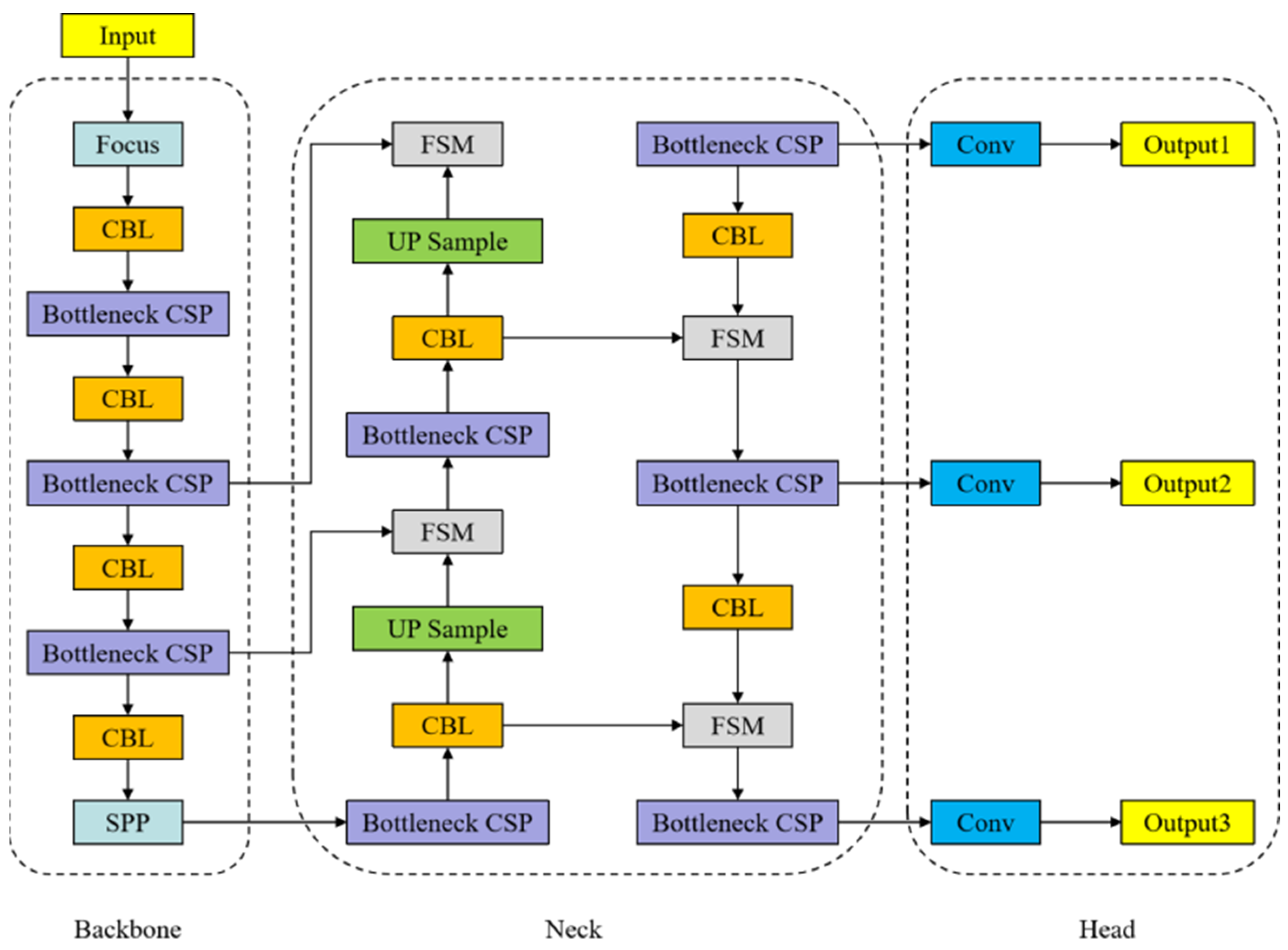
3.1. YOLO v5 Algorithm Improvements

The neck layer of the YOLO v5 algorithm mainly uses the Feature Pyramid Network (FPN) and Path Aggregation Network (PAN) structures. In 2017, Tsung-Yi Lin et al. pioneered the introduction of FPN [12]. FPN combines multi-scale features through a top-down hierarchical structure. The top-level features are up-sampled and fused with the bottom-level features. In this way, FPN obtains high-resolution and strong semantic features. However, FPN only passes the semantics from the top layer to the bottom layer. It does not pass the location information of the bottom layer feature map to the top layer. Therefore, the information of the top layer predictive feature map is not perfect. PAN adds a bottom-up, hierarchical structure and cross-layer connectivity with the same horizontal layer on the basis of FPN. It can pass the bottom layer’s feature information to the top layer’s predictive feature map effectively. Although this structure has many advantages, this method ignores a lot of redundant and conflicting information generated via direct the fusion of features of different scales. It limits the ability of original multi-scale representation. Therefore, we improved the neck layer with the FSM module [13] instead of the Concat module in this paper. The purpose was to filter conflict information. And this approach can prevent the special-case features from being overwhelmed due to conflicting information. The structure of the improved algorithm is shown in Figure 1.

As can be seen from Figure 1, the input images first enter the focus module for slicing. The regions of each slice are staggered at a certain interval to obtain the features after slicing. The feature output after slicing and combining is sent to the CBL module for convolution output; then, it enters the Bottleneck CSP module. The module structure divides the input into two parts. Part of it carries out the feature extraction of the Bottleneck branch. The other part transits through a convolution layer, and finally, it stacks in depth. The main purpose of the CSP structure is to enrich the realization of a feature learning network and reduce the memory occupation by nearly half. Similarly, the output from the first CSP module enters the CBL and CSP modules twice, and the output is bridged to a cascade structure deeper in the network at this moment. Then, it will enter the CBL and SPP modules. Because the input size becomes smaller after convolution at this moment, in particular, the extraction of small target features has gradually become difficult. Therefore, the SPP module was added to increase the maximum pooling operation of slices, and the multiple channels’ characteristics were significantly enhanced. The updated module realizes the high integration of global features and local features, and it enriches the expressive ability of feature maps. The following part is mainly intended to splice the features of the previous convolution operations. Because the input data dimension is different from the output data dimension, the dimension of the output becomes smaller. Starting from the first CSP module, the dimensions are cascaded through convolution, up-sampling, and other operations. The three outputs shown were obtained respectively. Three outputs were convolved as the input of network structure prediction. Three output detection results were obtained respectively. In order to filter the conflict information achieved via different levels of feature map fusion, a feature specify module (FSM) is proposed to replace the original Concat module. The general structure of the FSM is shown in Figure 2.

As we can see from Figure 2, this module primarily consists of two branches: a channel filtering branch and a spatial filtering branch. The spatial and channel-adaptive weights are generated through two branches. The spatial and channel-adaptive weights can guide the features to learn in more important directions. In order to determine the channel attention, the channel filtering branch compresses the input feature map in the spatial dimension so that the model only focuses on the dimension of the channel and aggregates the spatial information that can represent the image global features. By combining adaptive average pooling and adaptive maximum pooling, more fine-grained image global features are obtained. Suppose Xm is the input of the FSM (m = {1, 2}) layer, X(n,m) is the result of resizing the feature map from the nth layer to the mth layer, and $X_{k,x,y}^m$ is the value of the feature map at position (x, y) on the mth feature map in the kth channel [13]. Then, the output of the above branch is shown in Equation (1). In Equation (1), $K_{x,y}^m$ denotes the output vector of the mth layer at position (x, y). In Equation (1), a and b are the channel-adaptive weights of size 1 × 1 × 1. In Equations (2) and (3), a and b are defined.

$$K_{x,y}^m=a^m·X_{x,y}^{\left(1,m\right)}+b^m·X_{x,y}^{\left(2,m\right)}$$

(1)

$$a^m=\sigma \left[AP\left(F_1\right)+MP\left(F_1\right)\right]$$

(2)

$$b^m=\sigma \left[AP\left(F_2\right)+MP\left(F_2\right)\right]$$

(3)

F is the feature generated via splicing in Figure 2. σ denotes the Sigmoid operation. AP and MP represent average pooling and maximum pooling operations. Then, we sum these two weights across the spatial dimension to generate channel-based adaptive weights through the Sigmoid function. The spatial filtering branch generates the relative weights of each position with respect to the channel through Softmax. Its output is shown in Equation (4). In Equation (4), x and y denote the spatial locations of the feature mapping, ${\varphi }_{x,y}^m$ is the output feature vector at the (x, y) location, and ${\mu }_{c,x,y}^m$ and ${\upsilon }_{c,x,y}^m$ denote the spatial adaptive weights relative to the m-layer, where c denotes their channels. μ and υ are shown in Equation (5) and Equation (6). F in Equation (5) has the same meaning as Equation (2). The relative weights of different channels at the same location are obtained by normalizing the feature maps in the channel directions using Softmax [13]. Thus, the total output of the module can be expressed as Equation (7). In this way, the final features are fused on the basis of adaptive weights, and {p1, p2, p3, p4} are the final outputs of the whole network [14].

$${\varphi }_{x,y}^m={\displaystyle \sum }_{c=1}^2{\displaystyle \sum }_{c,x,y}\left({\mu }_{c,x,y}^m·X_{c,x,y}^{\left(1,m\right)}+{\upsilon }_{c,x,y}^m·X_{c,x,y}^{\left(2,m\right)}\right)$$

(4)

$${\mu }^m=Softmax\left(F_1\right)$$

(5)

$${\upsilon }^m=Softmax\left(F_2\right)$$

(6)

$$p_{x,y}^m={\varphi }_{x,y}^m+K_{x,y}^m$$

(7)

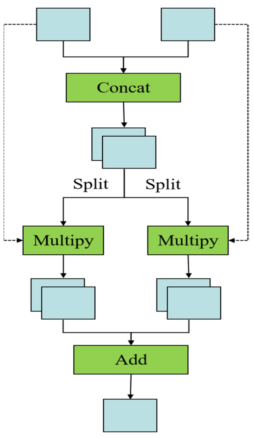
3.2. Model Optimization and Improvement

Aiming at the problems of false alarms and missed detection in the model, the factors that affect the ship detection results are as follows: the selection of the Confidence (conf) threshold, the setting of Intersection Over Union (Iou) threshold, and the setting of the learning rate. The conf threshold is intended mainly to exclude the detection results with confidence below the threshold. If the value is too high, the detection will be missed. If it is too low, a false alarm will appear. The Iou threshold is an important parameter in the non-maximal suppression method. When the network model extracts candidate regions from the image, multiple prediction boxes will appear for the same target. The purpose of non-maximal suppression is to sort the repeated prediction boxes by confidence in order to filter out an optimal box. The value of Iou is equal to the ratio of the intersection area and union area of the two prediction boxes. When the ratio is higher than the Iou threshold, the two prediction boxes are identified as the same target.

We used the control variable method. The parameters of conf and Iou were adjusted using the verification set. First, we controlled the Iou threshold to 0.4 and tested the optimal conf threshold, as shown in

Table 1. Test results of different Conf thresholds (the Iou threshold was 0.4).

Conf Threshold	Number of Detections	Number of Missed Detections	False Alarm Number	Test Set	Detection Rate	False Alarm Rate
0.8	183	117	0	Positive samples: 300 Negative samples: 29	61.0%	0
0.7	236	64	2		78.7%	6.9%
0.6	265	35	5		88.3%	17.2%
0.5	292	8	9		97.3%	31.0%

. We found that the detection rate and false alarm rate also changed when the conf threshold changed. Of course, we needed a higher detection rate and a lower false alarm rate [15]. So, we subtracted the false alarm rate from the detection rate to get a difference. The larger the difference, the better. From Table 1, we can see the difference under different threshold conditions: when the Conf threshold was 0.8, the difference was 61%; when the Conf threshold was 0.7, the difference was 71.8%; when the Conf threshold was 0.6, the difference was 71.1%; and when the Conf threshold was 0.5, the difference was 66.3%. We found that, when the Conf threshold was 0.6 and 0.7, the difference was greater than 71%. At this time, we should account for the percentage of the correct quantity detected. When the Conf threshold was 0.7 and 0.6, the percentage of the correct quantity detected was 78% and 86.7%. Obviously, the Conf threshold of 0.6 is better. Similarly, we controlled the conf threshold to 0.5 and tested the best Iou threshold, as shown in

Table 2. Test results of different Iou thresholds (the Conf threshold was 0.5).

Iou Threshold	Number of Detections	Number of Missed Detections	False Alarm Number	Test Set	Detection Rate	False Alarm Rate
0.6	274	26	11	Positive samples: 300 Negative samples: 29	91.3%	37.9%
0.5	256	44	7		85.3%	24.1%
0.4	215	85	3		71.7%	10.3%
0.3	196	104	1		65.3%	3.4%

. The difference between the detection rate and the false alarm rate was also obtained: when the Iou threshold was 0.6, the difference was 53.4%; when the Iou threshold was 0.5, the difference was 61.2%; when the Iou threshold was 0.4, the difference was 61.4%; and when the Iou threshold was 0.3, the difference was 61.9%. When the Conf threshold was 0.5, 0.4, and 0.3, the difference was greater than 61%. At this time, we should also consider the percentage of the correct quantity. When the Iou was 0.5, 0.4, and 0.3, the percentage of the correct quantity was 83%, 70.7%, and 65%. Obviously, the Iou threshold of 0.5 is better. When the detection rate and false alarm rate were considered comprehensively, a balance was found between them. The value of Conf was 0.6, and the value of Iou was 0.5. Then, we used this parameter setting to perform another test. Compared with the improved model, the detection rate and false alarm rate were optimized, as shown in

Table 3. Comparison of detection effects before and after optimization.

Numbering	Algorithm Type	Detection Rate	False Alarm Rate
1	before optimization	81.7%	19.8%
2	after optimization	83.5%	11.2%

. It can be seen that, after this improvement, the false alarm rate was reduced, and the detection rate was also slightly improved. The overall performance was improved.

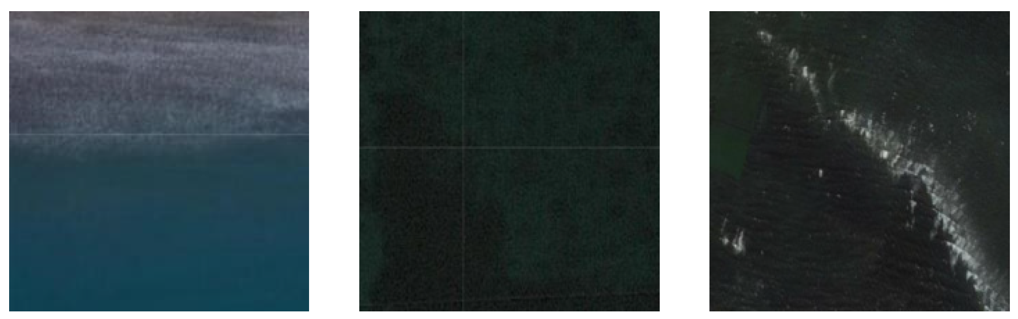
3.3. Image Data Enhancement

Deep learning methods often require a large amount of data, but the data sources of ship remote sensing images are limited. The time cost of targets’ manual interception is quite high. Data sets often cannot meet the training requirements, so data enhancement methods are required. It has two functions. The first function is to expand the data set and improve the model performance. The second function is to enhance the noise and improve the network’s robustness [16,17].

There are two data enhancement methods for pixel-level adjustments: The first method is to achieve light distortion by changing the brightness, contrast, and saturation, as shown in Figure 3. The second method is geometric distortion, including random scaling, rotation, cropping, and other methods. In addition to pixel-level data enhancement, there are also image occlusion methods, such as random erasing.

The data enhancement method using the YOLO v5 algorithm is a mosaic method, which can piece up multiple images randomly into one picture for training. The new image includes more target information and more complex background information, which can improve the robustness of the network effectively. The enhanced data set is 8 times larger than the original data set. A schematic diagram of the mosaic data enhancement method is shown in Figure 4.

4. Data Set and Implementation Settings

Ship target detection plays a vital role in task implementation for various fields. The ocean surveillance system can obtain sea surface images through remote sensing satellites, which can monitor the ocean for 24 h a day. The computer can detect ships from the remote sensing images automatically [18,19,20]. This paper takes nine types of major ships disclosed as examples for research, which is of great significance to the improvement of automatic target detection technology for ships.

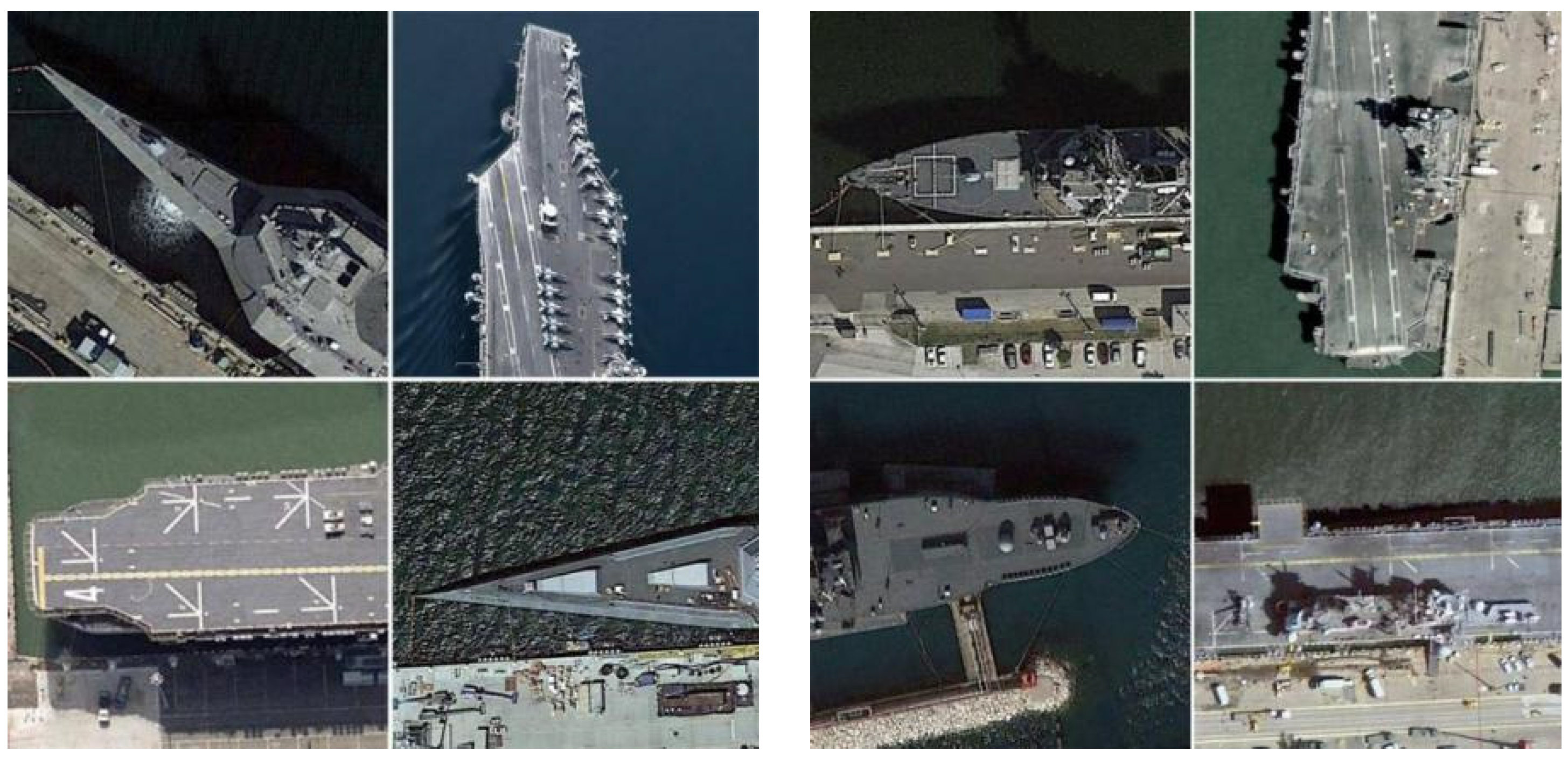
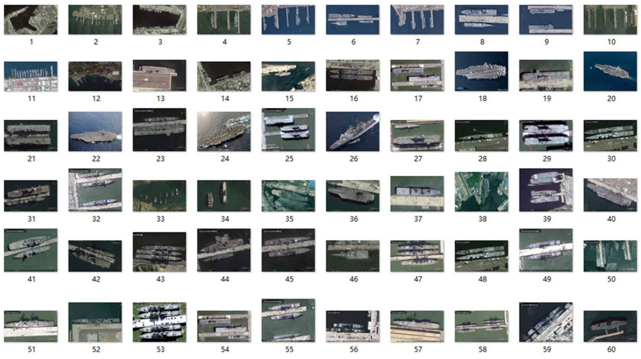
4.1. Remote Sensing Ship Data Set Acquisition

Deep neural networks require a lot of samples for training. At the same time, ship detection tasks face complex factors such as changeable weather, backgrounds, and so on, which need a large amount of data to enhance the anti-interference capability. So, obtaining sufficient sample data has become the key task for successful detection. In this paper, the High Resolution Ship Collection (HRSC) data set and self-made data set were selected. The HRSC data set is collected by Northwestern Polytechnical University, and it includes ships at sea and along the coast. The image resolution is between 0.4 and 2 m. At the same time, we also collected a self-made data set of ships from public, high-resolution remote sensing images. The statistics of the ship detection data sets are shown in

Table 4. Statistics of ship detection data sets.

Name of the Ship	Training Set	Validation Set	Test Set	Number of Images
Nimitz class	135	38	19	192
Ticonderoga class	273	78	39	390
Zumwal class	39	11	5	55
Arleigh Burke class	307	88	44	399
Perry class	41	12	6	59
Independent class	184	52	26	262
Free class	149	42	21	212
Wasp class	122	35	17	174
San Antonio class	118	34	17	169
Total	1368	390	194	1952

.

In most cases, the approach involves near-shore ships’ target detection when a ship is moored at a pier. That process can be affected due to the adjacent pier and near-shore buildings. The automatic target detection can be disrupted [21,22]. Therefore, the target interception of major ports covered 98% of ships when the data set was built up. The data came from open, high-definition remote sensing images and manually intercepted ship remote sensing images with different weather, different coordinates, different directions, and different scales. In addition, there were related pictures collected from the internet, which constitute a data set of 1952 images. The obtained data set was divided into a training set (for learning), a validation set (for setting hyperparameters), and a test set (for testing prediction effects) with a ratio of 7:2:1. The total number of pictures is 1952, and the total number of ships is 4652, resulting in an average of 2.4 ship targets per picture [23]. Some samples are shown in Figure 5. In addition, in order to reduce the marine background interference in ship detection, background pictures were also intercepted as negative samples, which can not only improve the detection accuracy but also reduce the false alarm rate. Some background pictures are shown in Figure 6.

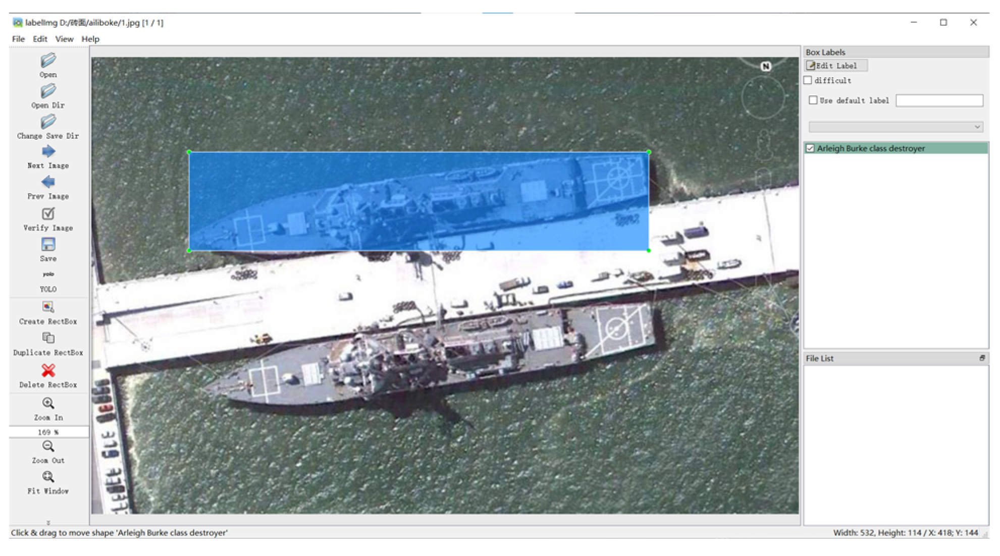
4.2. Data Set Ship Target Labeling

The Anaconda prompt command line was used, and labelImg was adopted for data labeling, which is shown in Figure 7. The horizontal labeling box was used to label ship targets. When labeling was conducted, the prediction box contracting the non-target part was avoided as much as possible, which can circumvent the background interference of network training [24]. For example, when labeling ships moored in port is conducted, the prediction box should avoid the dock part to more clearly distinguish between the background and the target.

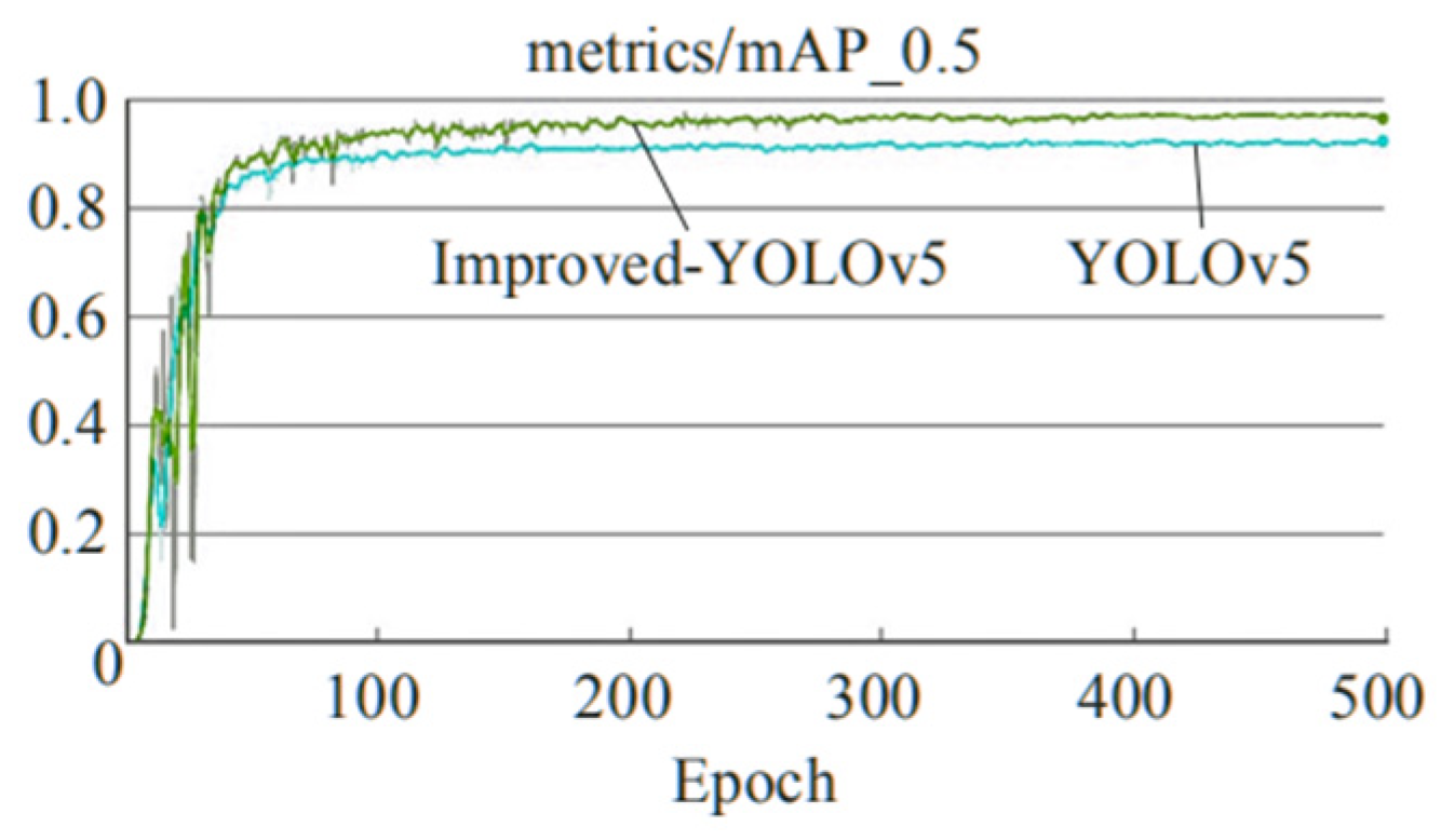
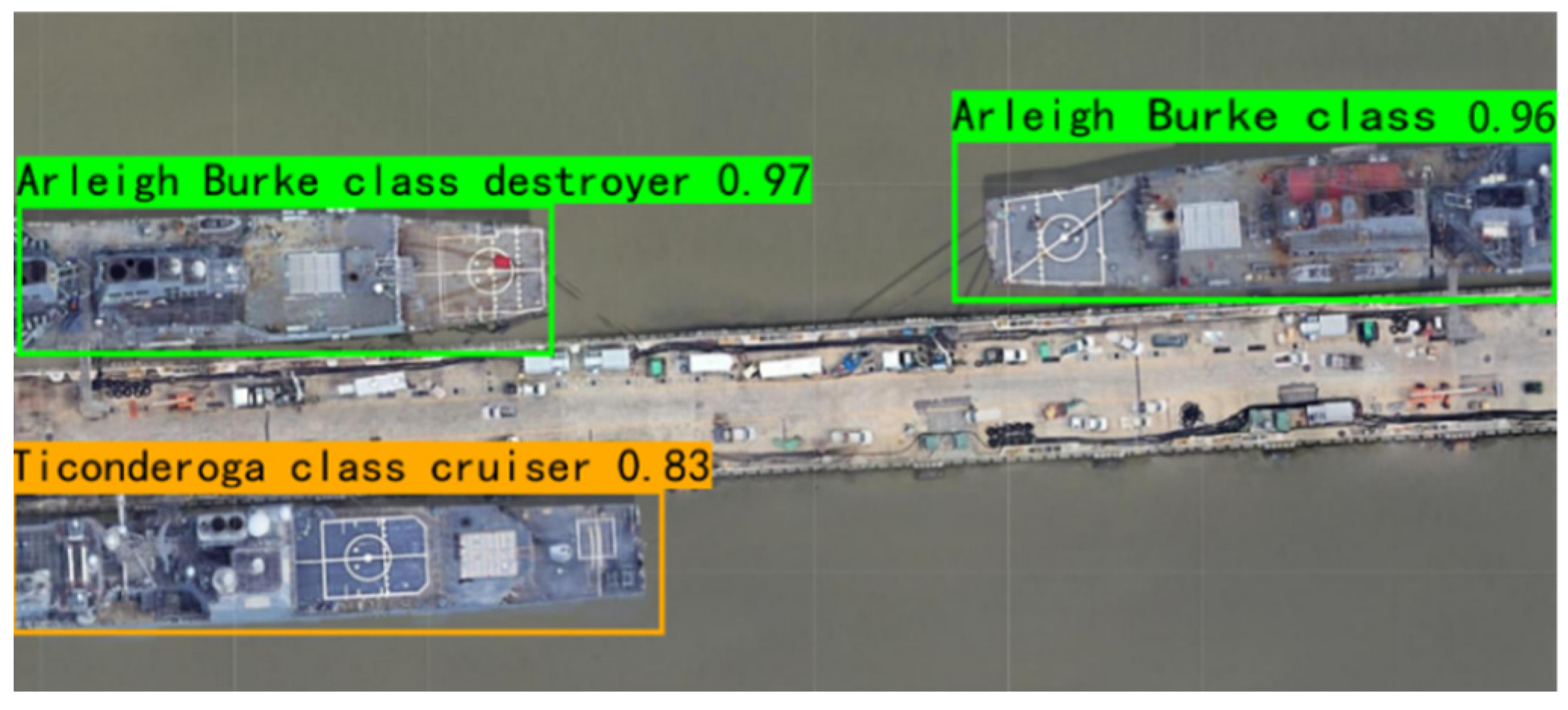
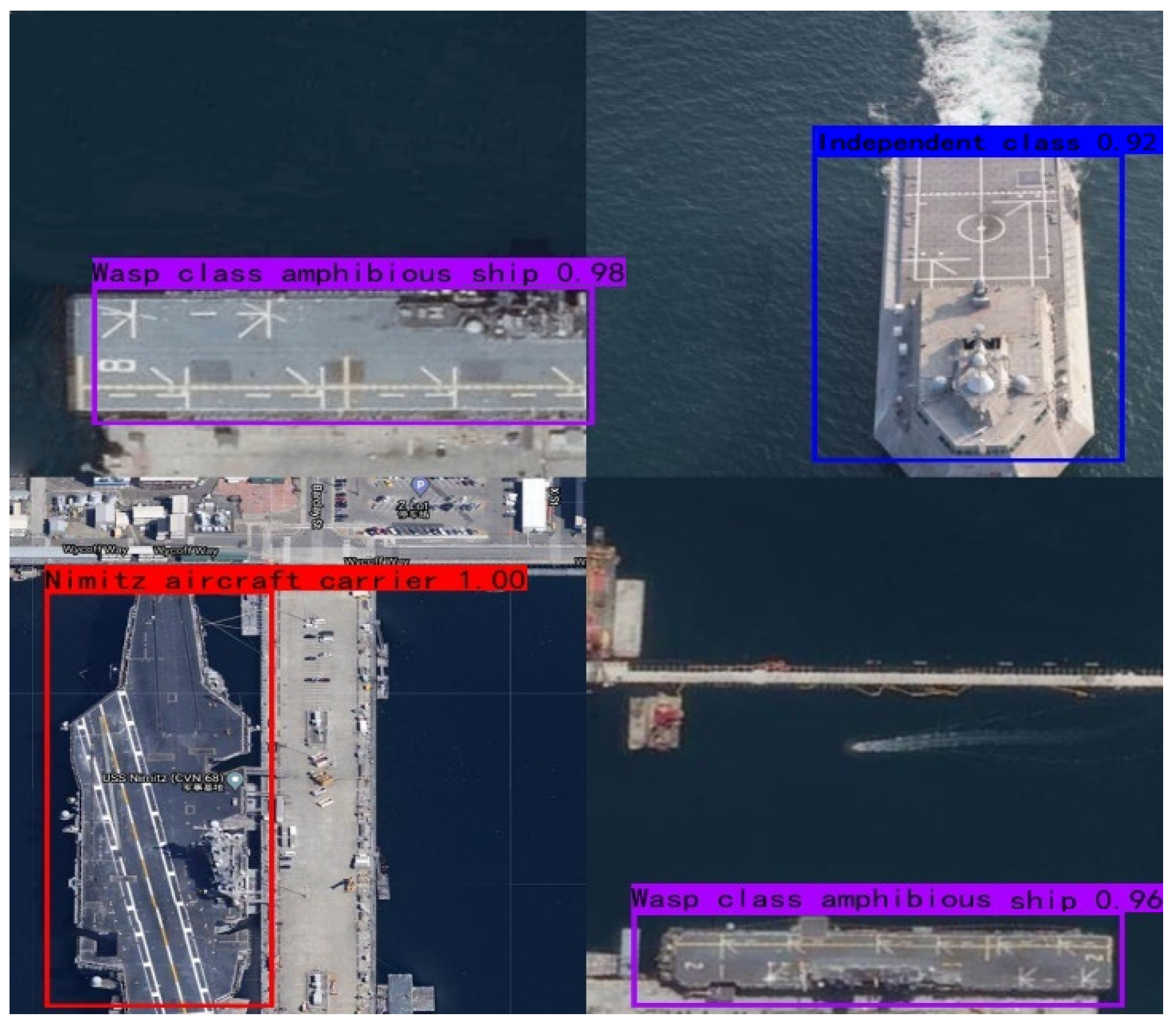
5. Experiments and Results

5.1. Implementation Settings

Using the idea of transfer learning, the weight was regarded as the initial value for the ship target detection model, which was trained as an open-source model. It can accelerate the training process of the network. The experimental environment was a Windows system, the GPU was configured with GTX1050Ti, the learning rate was set to 0.01, the label smoothing was 0.005, the training generation was 100, and the mosaic data enhancement was used.

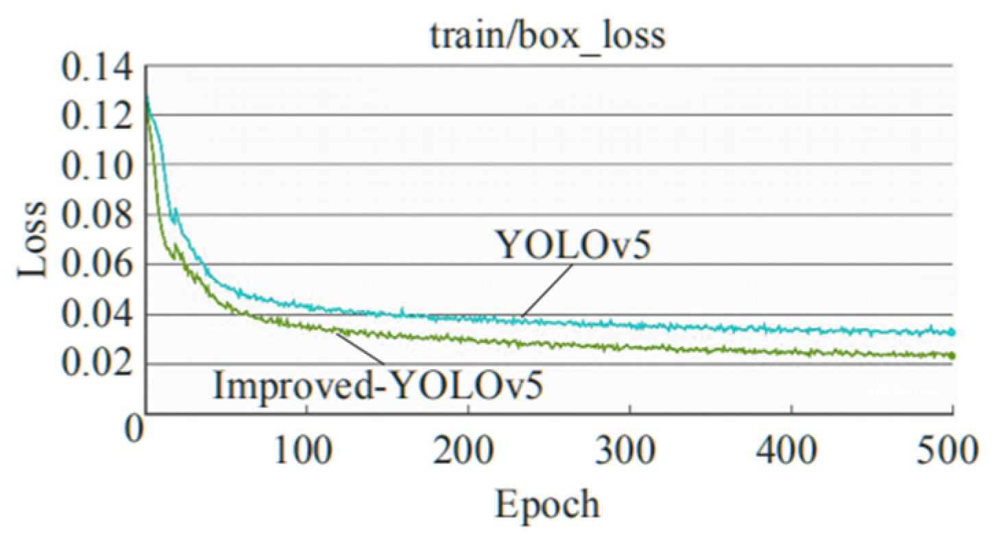
5.2. Pre-Training and Training Details

The VOC weight file was adopted for the pre-training weight. There are four pictures per training cycle, each with a 416 × 416 image processing size. Each time an epoch was trained, a weight file was automatically generated for the system. It can record the update of weight parameters after the current round of training has been completed [25]. The loss curve is shown in Figure 8. The horizontal coordinate is the number of epoch training times. The vertical coordinate is the loss value of the predicted edges. The loss value gradually decreased with the training process. The recognition ability of the network model also improved, which indicated that the network converged towards the real situation. The boundary loss value curve of the improved YOLO v5 demonstrated better convergence properties during its descent. Figure 9 shows the curve of the Mean Average Precision (mAP) index when the threshold of Iou was 0.5. The mAP value of the improved YOLO v5 is significantly better than that of the original algorithm.

When the confidence was set to 0.5, multiple prediction boxes will appear for the same target, showing detection results with low confidence. This situation can be effectively avoided by raising the threshold appropriately according to the model performance. Figure 10 adjusts the threshold to 0.6 to effectively filter out erroneous detection results.

The model performance can be directly affected due to the number of training rounds. In Figure 11, 50 rounds of training were finished. With the weight of the fiftieth round for prediction, there were many missed detection situations. With the increase in the number of training rounds, the loss value continued to converge. The model detection effect was greatly improved after the training parameters were adjusted [26].

In order to evaluate the detection performance of the improved YOLO v5 method, a quantitative comprehensive evaluation was made in an experiment, which adopted a variety of evaluation metrics from different angles.

Table 5. Comparison of the improved algorithm with other algorithms.

Method	Recall	Precision	mAP
Faster R-CNN	68.5%	72.8%	69.7%
SSD	74.9%	76.8%	75.7%
YOLO v4	75.9%	78.3%	77.6%
YOLO v5	79.4%	80.5%	79.7%
Improved YOLO v5	80.1%	82.7%	81.4%
YOLO v7	79.6%	81.2%	80.1%
YOLO v8	80.1%	82.1%	80.9%

shows the detection results of the improved module and other mainstream detection methods. It can be seen from the table that the recall, precision, and mAP of the improved YOLO v5 test reached 80.1%, 82.7%, and 81.4%, which was significantly better than Faster R-CNN, SSD, YOLO v4, and YOLO v5. In this way, the target detection accuracy was improved. As can be seen from Table 5, the improved YOLO v5 algorithm and YOLO v8 algorithm achieved higher recall, precision, and mAP than YOLO v7 because YOLO v8 has more convolution layers and parameters than YOLO v7, which makes YOLO v8 extract features better in some complex scenes at sea. And the improved YOLO v5 algorithm effectively filters the conflict information of the sea and refines the ship features to improve the accuracy of ship detection. Therefore, the improved YOLO v5 and YOLO v8 algorithms are more excellent in ship detection. Finally, we compared the improved YOLO v5 with YOLO v8. The recall of the improved YOLO v5 and YOLO v8 algorithms was both 80.1%. But the precision of the improved YOLO v5 algorithm was 82.7%, which is higher. This means that the improved YOLO v5 model has a lower false alarm rate, especially for ship target detection in a complex environment. The improved YOLO v5 has better robustness.

The precision and recall (P-R curves) of YOLO v5 and improved YOLO v5 are shown in Figure 12. By analyzing and comparing the precision and recall (P-R curves) of the models, it can be found that the vertical coordinate precision represents its correct rate of segmenting out for vehicle targets. The horizontal coordinate recall represents the ability of the network model to segment out all the vehicle targets in the image. Ideally, the P-R curve is a straight line with a precision of 1 at all times. A well-performing model can keep the precision at a high value while the recall is growing. A poorly performing model needs to sacrifice a lot of precision value in exchange for an increase in recall. The P-R curve of the improved YOLO v5 model was above that of the YOLO v5 model. The recall was higher for the same checking precision. The detection ability for ship targets is obviously promoted through the improved YOLO v5 model.

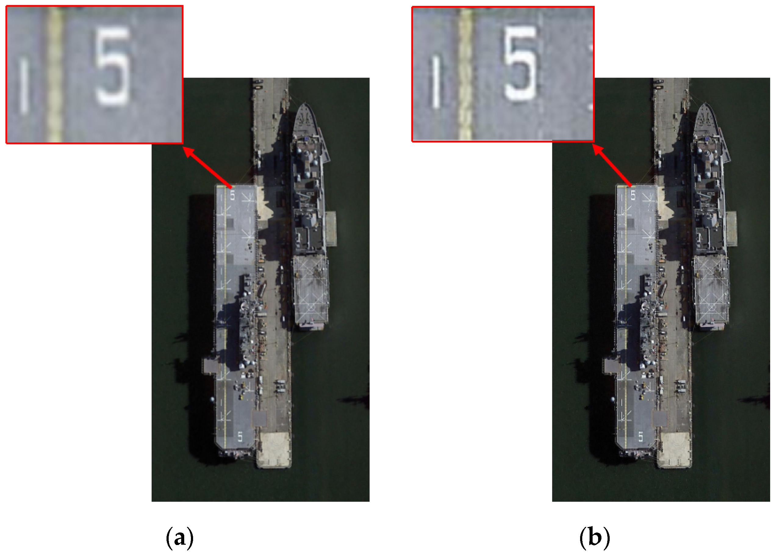
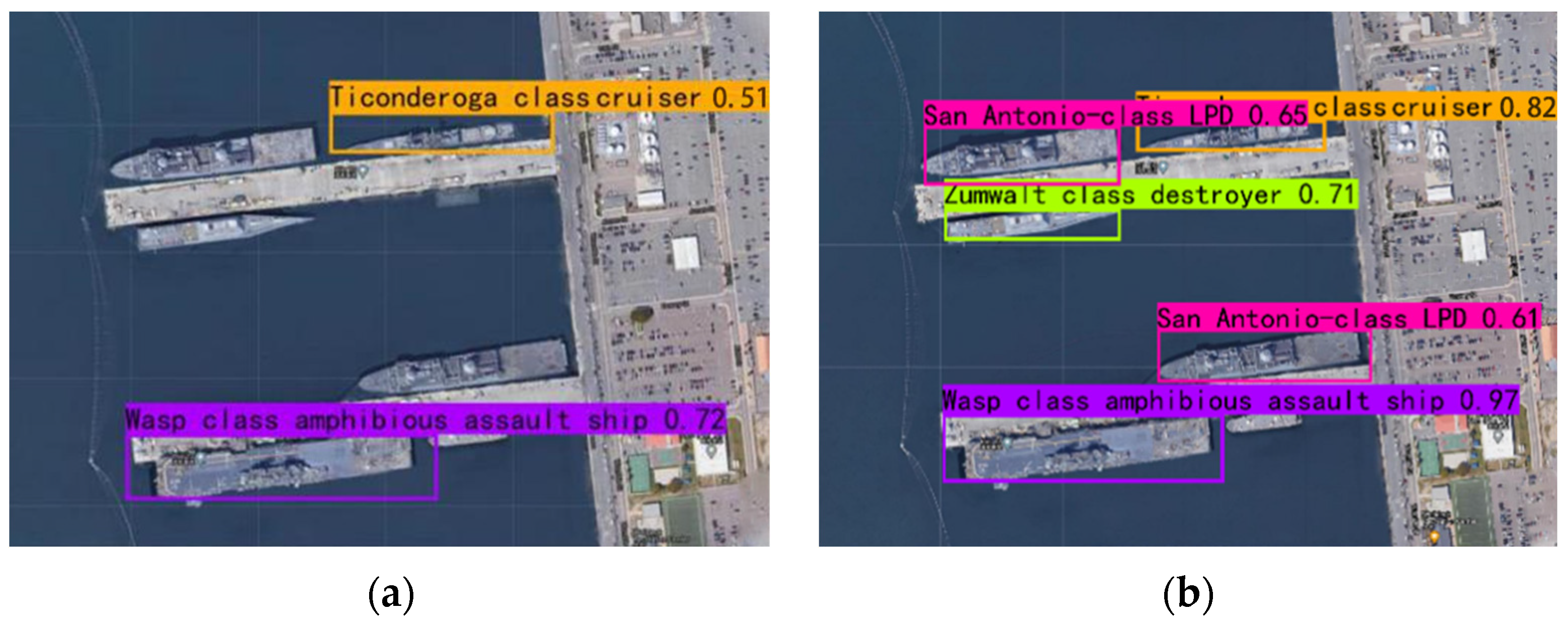
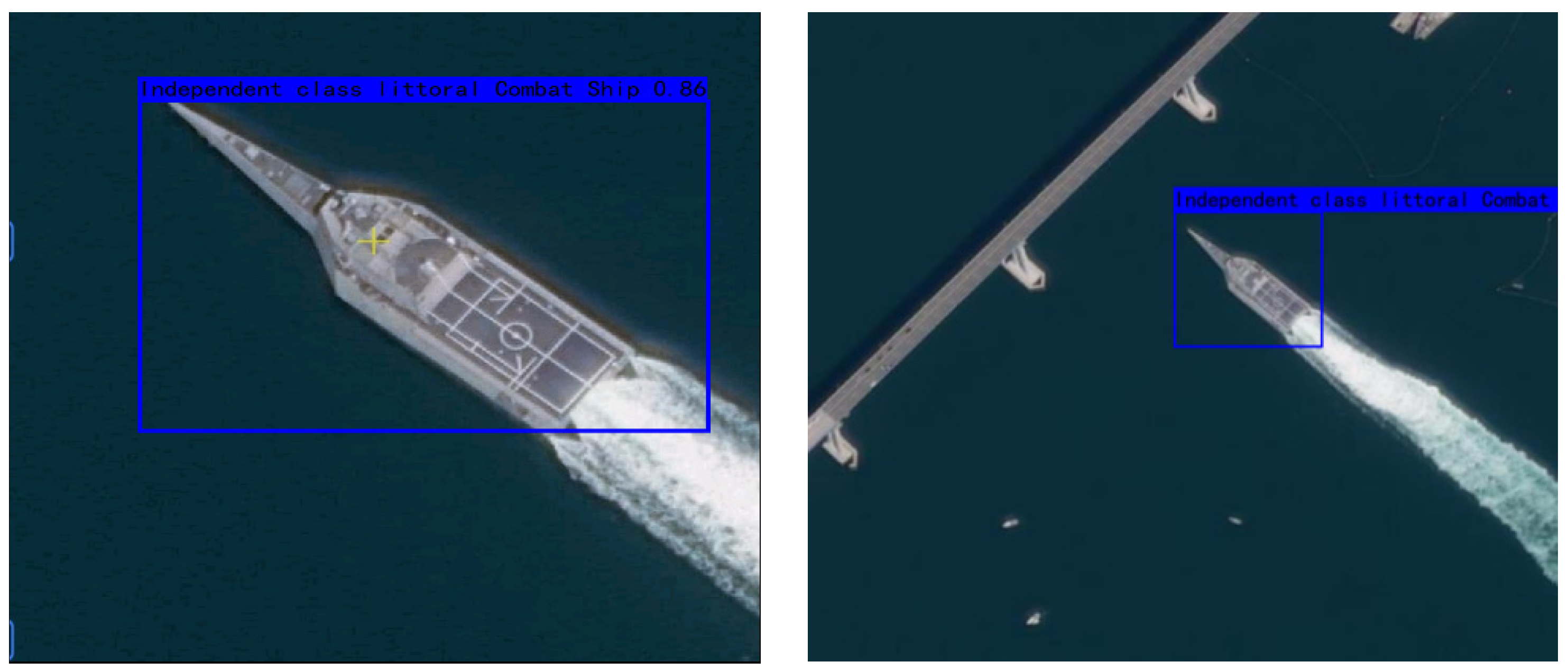
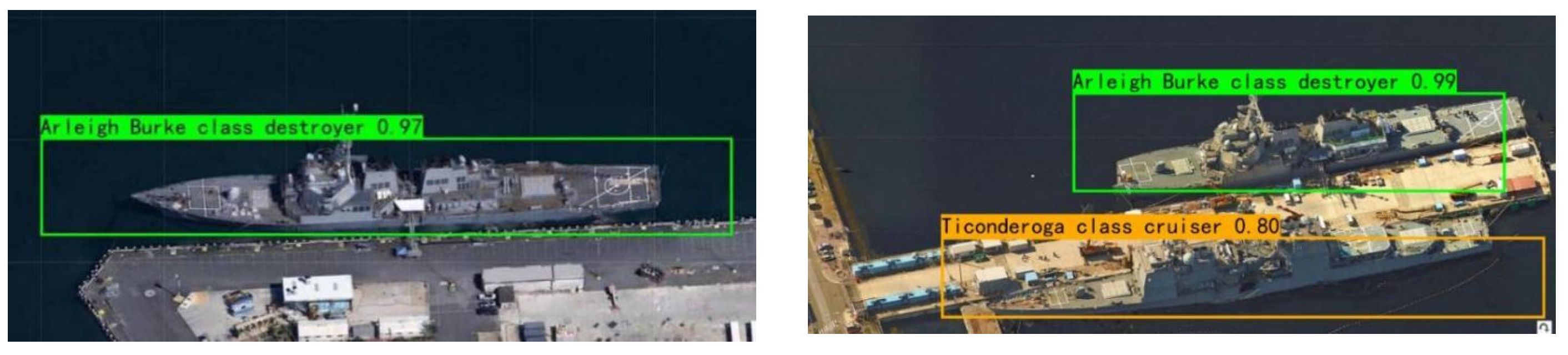
5.3. Robustness Testing

The loss value was 0.8 after training converged. The prediction effect was quite good after the test set finished testing. Accurate predictions can be made under different degrees of interference.

The detection effect of targets at different scales revealed that the trained model can detect images at different scales, as shown in Figure 13, in which the detection of large-scale and small-scale images of the same target is compared [27].

The detection effect of oblique targets mainly detects the top features of ships. The experimental data set was based on remote sensing images. The oblique images were put into the model for prediction. It was verified that the robustness was good, as shown in Figure 14. Therefore, this model can be transferred to target detection for aerial imagery [28,29,30].

The detection effect of incomplete targets has always been a problem in the target detection field because only the local part of the target can be shown, so it is difficult for the network to collect the target-complete features. The detection effect of an incomplete target is also one of the important indicators to measure the robustness of the model. In Figure 15, only the stern parts of the three ships are shown, but they can still be accurately detected with confidence levels of 0.97, 0.96, and 0.83, respectively. In Figure 16, the four images are randomly pieced up according to mosaic data enhancement, and only local parts of the four targets are retained. The network could still detect very well [31,32].

5.4. Algorithm Evaluation Indicators

As can be seen from

Table 6. Ship test results.

Category	TP	FP	Missed Detection	Total Samples	Recognition Rate
Nimitz class	163	26	3	192	84.9%
Ticonderoga class	348	27	15	390	89.2%
Zumwal Class	39	11	5	55	70.9%
Arleigh Burke class	360	22	17	399	90.2%
Perry class	44	12	3	59	74.6%
Standalone level	226	20	16	262	86.3%
Free class	160	35	17	212	75.5%
Wasp class	136	21	17	174	78.1%
San Antonio class	118	26	15	169	69.8%
Total	1594	200	108	1952	81.7%

, the average identification rate reached 81.7%. The Arleigh Burke-class destroyers had the highest detection accuracy among the nine types of ships considered. The network is more inclined to such targets because of their larger sample size [33].

6. Conclusions

Traditional target detection methods have many drawbacks. The manual design features do not achieve good robustness. They are often disturbed due to complex backgrounds and other factors. Therefore, their detection is ineffective. The process of a target detection algorithm based on deep learning was improved: in area selection, the deep learning target detection algorithm abandons the traditional sliding window strategy. It uses a series of algorithms to find the possible target area as a candidate area, which greatly improves the detection speed at the feature extraction stage. There is no need to manually design features like traditional detection, but the convolution kernel of convolutional neural networks was used to independently extract features, which not only realizes the end-to-end structure but also has a stronger expression ability for features and improves robustness. In this paper, nine classes of ships were used as samples. The different ship remote sensing images were intercepted or collected via the network. The YOLO v5 model was used for training. The effective features were analyzed and extracted from massive remote sensing image data. The task of ship targets’ automatic detection was realized in complex marine and coastal environments.

References

1. Xu, C.; Wang, X.; Yang, Y. Attention YOLO: YOLO Detection Algorithm Introducing Attention Mechanism. Comput. Eng. Appl. 2019, 55, 13–23. [Google Scholar]
2. Liu, X. Research on Image Object Detection Algorithm Based on YOLO Deep Learning Model. Comput. Program. Ski. Maint. 2022, 7, 131–134. [Google Scholar]
3. Shuai, T.; Sun, K.; Wu, X.; Zhang, X.; Shi, B. A Ship Target Automatic Detection Method for High-resolution Remote Sensing. In Proceedings of the Geoscience & Remote Sensing Symposium, Beijing, China, 10–15 July 2016; IEEE: Piscataway, NJ, USA, 2016; pp. 1258–1261. [Google Scholar]
4. Peng, D.; Ye, Z.; Ping, J. Ship Detection on Sea Surface Based on Multi-feature and Multi-scale Visual Attention. Opt. Precis. Eng. 2017, 25, 2461–2468. [Google Scholar] [CrossRef]
5. Liu, Y.; Cui, H.; Li, G. A Novel Method for Ship Detection and Classification on Remote Sensing Images. In 2017 International Conference on Artificial Neural Networks; Springer: Cham, Switzerland, 2017; pp. 556–564. [Google Scholar]
6. Zhao, Q. Ship Target Recognition Research Based on Multi Physics Field Features; Harbin Institute of Technology: Harbin, China, 2017. [Google Scholar]
7. Klepko, R. Classification of SAR Ship Images with Aid of a Syntactic Pattern Recognition Algorithm; Defence Research Establishment Ottawa: Ottawa, ON, Canada, 1991. [Google Scholar]
8. Wang, B. Research on Deep Learning-Based Ship Detection; Xiamen University: Xiamen, China, 2017. [Google Scholar]
9. Yuan, Y.; Jiang, Z.; Zhao, D. Ship Detection in Optical Remote Sensing Images based on Deep Convolutional Neural Networks. J. Appl. Remote Sens. 2017, 11, 135–149. [Google Scholar]
10. Wang, T. Ship Detection Technology in High Resolusion Remote Sensing Image Using Deep Learning; Harbin Institute of Technology: Harbin, China, 2017. [Google Scholar]
11. Liu, Y. Research on Ship Detection from High-Resolution Optical Remote Sensing Images; Xiamen University: Xiamen, China, 2017. [Google Scholar]
12. Lin, T.Y.; Dollar, P.; Girshick, R.; He, K.; Hariharan, B.; Belongie, S. Feature Pyramid Networks for Object Detection. In Proceedings of the IEEE Conference on Computer Vision and Pattern Reconstruction, Columbus, OH, USA, 23–28 June 2014; pp. 2117–2125. [Google Scholar]
13. Yu, J.; Jia, Y. Improving YOLOv5’s Small Object Detection Algorithm. Comput. Eng. Appl. 2023, 59, 203–204. [Google Scholar]
14. Xiao, J.J. Masked face detection and standard wearing mask recognition based on YOLOv3 and YCrCb. Comput. Eng. Softw. 2020, 41, 164–169. [Google Scholar]
15. Huang, F.; Chen, M.; Feng, G. Improved YOLO object detection algorithm based on deformable convolutions. Comput. Eng. 2021, 47, 269–275. [Google Scholar]
16. Song, Z.; Sui, H.; Li, Y. Overview of Ship Target Detection in High Resolution Visible Light Remote Sensing Images. J. Wuhan Univ. (Inf. Sci. Ed.) 2021, 11, 1703–1715. [Google Scholar]
17. Wang, Q. Introduction to Deep Learning: Theory and Implementation Based on Python; People’s Posts and Telecommunications Press: Beijing, China, 2018. [Google Scholar]
18. Xu, C.; Cheng, W.; Yang, Y. Basic Research on YOLO Object Detection Algorithms. Comput. Inf. Technol. 2020, 28, 45–47. [Google Scholar]
19. Long, F.; Wang, Y. Introduction and Practice of Deep Learning; Tsinghua University Press: Beijing, China, 2017. [Google Scholar]
20. Li, J.; Qu, C.; Peng, S.; Deng, B. SAR Image Ship Target Detection Based on Convolutional Neural Network. Syst. Eng. Electron. 2018, 40, 1953–1959. [Google Scholar]
21. Yang, Y. Ship Target Detection and Classification Recognition Based on Deep Learning. Master’s Thesis, Huazhong University of Science and Technology, Wuhan, China, 2019. [Google Scholar]
22. Yasuhiri, S. Introduction to Deep Learning Based on the Theory and Implementation of Python; China Industry and Information Technology Publishing Group: Beijing, China, 2021. [Google Scholar]
23. Zhang, Y. Research on Intelligent Detection and Recognition of Ship Targets on the Sea Surface in Optical Images; University of Chinese Academy of Sciences: Beijing, China, 2021. [Google Scholar]
24. Xu, Z.; Ding, Y. Ship target detection in remote sensing images using adaptive rotating region generation network. Prog. Laser Optoelectron. 2020, 57, 408–415. [Google Scholar]
25. Liu, J.; Li, Z.; Zhang, X. Overview of Sea Surface Target Detection Technology in Visible Light Remote Sensing Images. Comput. Sci. 2020, 3, 116–123. [Google Scholar]
26. Li, Q. Research on Target Detection Methods of Fast and Efficient Deep Neural Network. Master’s Thesis, Beijing Jiaotong University, Beijing, China, 2019. [Google Scholar]
27. Ye, Q.; Zha, X.; Li, H. High resolution remote sensing image ship detection based on visual saliency. Ocean. Surv. Mapp. 2018, 38, 48–52. [Google Scholar]
28. Yan, Y. Image Recognition of Deep Learning: Core Technology and Case Practice; China Machine Press: Beijing, China, 2019. [Google Scholar]
29. Wang, Y.; Ma, L.; Tian, Y. Overview of Ship Target Detection and Recognition in Optical Remote Sensing Images. J. Autom. 2011, 9, 1029–1039. [Google Scholar]
30. Zhao, H.; Wang, P.; Dong, C.; Shang, Y. Ship target detection based on multi-scale visual salliency. Opt. Precis. Eng. 2020, 6, 1395–1403. [Google Scholar] [CrossRef]
31. Dong, C.; Liu, J.; Xu, F.; Wang, R. Rapid detection method for ship targets in optical remote sensing images. J. Jilin Univ. (Eng. Ed.) 2019, 49, 1369–1376. [Google Scholar]
32. Sun, L.; Jiang, Y.; Wang, J.; Xiang, B. Pytorch Machine Learning from Introduction to Practice; China Machine Press: Beijing, China, 2019. [Google Scholar]
33. Gai, S.; Bao, Z. High noise image denoising algorithm based on deep learning. J. Autom. 2020, 12, 2672–2680. [Google Scholar]
Figure 1. The improved YOLO v5 network structure. CBL denotes Convolution Batch Normalization and Leaky ReLU; CSP denotes Cross-Stage Partial; SPP denotes Spatial Pyramid Pooling; and FSM denotes Feature Specify Module.
Mathematics 12 01714 g001
Figure 2. Feature specify module (FSM).
Mathematics 12 01714 g002
Figure 3. MContrast image before and after image enhancement: (a) image before image enhancement; (b) image after image enhancement.
Mathematics 12 01714 g003
Figure 4. Schematic diagram of mosaic data enhancement.
Mathematics 12 01714 g004
Figure 5. Examples of a ship target data set.
Mathematics 12 01714 g005
Figure 6. Examples of background image data set.
Mathematics 12 01714 g006
Figure 7. Using image labeling tools to label ship targets.
Mathematics 12 01714 g007
Figure 8. Change in loss curve.
Mathematics 12 01714 g008
Figure 9. Change in mAP curve.
Mathematics 12 01714 g009
Figure 10. Comparison of test results before and after threshold adjustment: (a) the test result before threshold adjustment; (b) the test result after threshold adjustment.
Mathematics 12 01714 g010
Figure 11. Comparison of test results for 50 rounds of training and 100 rounds of training: (a) the training test result for 50 rounds; (b) the training test result for 100 rounds.
Mathematics 12 01714 g011
Figure 12. P-R curve.
Mathematics 12 01714 g012
Figure 13. Test result comparison of a target at different scales.
Mathematics 12 01714 g013
Figure 14. Detection effect of oblique targets.
Mathematics 12 01714 g014
Figure 15. Detection of incomplete targets.
Mathematics 12 01714 g015
Figure 16. Detection of randomly pieced-up images.
Mathematics 12 01714 g016