Event-Triggered Tracking Control for Nonlinear Systems with Mismatched Disturbances: A Non-Recursive Design Approach

Abstract

Considering the situation of limited resources in practical applications, it is significant to design control algorithms with high resource utilization rates for a class of nonlinear systems subject to mismatched disturbances. In contrast to common recursive methods, this paper proposes a novel event-triggered tracking control approach by co-designing the triggering event and the controller within a non-recursive design framework that combines disturbance estimation techniques and feedforward compensation strategies. Through rigorous Lyapunov stability analysis, the global boundedness of each state in the closed-loop system is demonstrated, and the absence of the Zeno phenomenon is further verified. A representative numerical simulation and a practical implementation for speed regulation of permanent magnet synchronous motor (PMSM) system confirm the effectiveness and simplicity of the proposed control strategy.

1. Introduction

In recent years, significant theoretical achievements have been made in addressing various nonlinear systems control problems (see, e.g., [1,2,3]). When considering the practical application of these advanced control algorithms, traditional sampled-data control methods [4,5] rely on a predetermined fixed sampling period derived from worst-case analyses. This approach might burden systems with limited computational and communication resources, such as network control systems and microprocessor-based systems. In response, event-triggered control strategies have emerged, employing specific ‘events’ to govern sampling and execution processes. By contrast, this method activates signal transmission and control updates only when necessary, potentially reducing the system redundancy and conserving the bandwidth resources while maintaining a satisfactory closed-loop performance, as referenced in [6].

Up to now, various results have been achieved in event-triggered control design for nonlinear systems. Previous studies introduce static and dynamic event-triggered stabilization frameworks in [7,8], respectively, assuming that the closed-loop system demonstrates input-to-state stability (ISS) with respect to sampling errors. Despite the proficiency of the ISS framework in handling system nonlinearity, integrating it with uncertainty compensation remains a challenge. Consequently, researchers are endeavoring to develop design schemes that, independent of the ISS assumption, integrate uncertainty management with flexible event-triggered compensation to achieve the desired control objective. In this direction, ref. [9] proposes an adaptive event-triggered tracking strategy employing dynamic gains derived from tracking errors, while [10] utilizes a similar approach to design an event-triggered output feedback controller, ensuring global stabilization for a class of uncertain systems. Furthermore, leveraging the backstepping technique, adaptive event-triggered state/output feedback control strategies have been developed. For example, ref. [11] introduces a decentralized event-triggered control strategy for a class of uncertain large-scale systems with unmodeled dynamics. Additionally, ref. [12] presents three practical tracking control strategies: fixed threshold, relative threshold, and switching threshold when systems containing unknown parameters.

In real-world scenarios, control systems are invariably affected by external disturbances. It is worth noting that the previously mentioned event-triggered control schemes lack analysis and active attenuation of system disturbances. Conventional anti-disturbance control strategies, as documented in [13,14], primarily focus on managing disturbances and ensuring system stability, but often overlook the communication and computation burdens imposed on the systems. Therefore, integrating research on control issues in disturbed systems with event-triggered methodology can effectively utilize limited resources for implementing advanced control algorithms in practical settings.

Undoubtedly, this integration poses significant challenges in designing compensation mechanisms and conducting system performance analysis within the confines of existing triggering mechanisms and anti-disturbance control conditions. For example, a PI-type tracking controller is proposed in [15] through the integration of disturbance estimation and triggered extended state techniques. Additionally, finite-time disturbance observers are employed to handle unmatched disturbances, and the technique of adding a power integrator is utilized to address the event-triggered tracking control problem, as discussed in [16]. However, this recursive-based control design may lead to the ‘explosion of terms’ problem, posing obstacles in their direct engineering application. To avoid the direct differentiation of virtual control laws, event-triggered schemes combined with command filtering techniques are proposed in [17,18]. Moreover, the investigation of event-triggered dynamic surface control strategy can be found in [19]. In contrast to the approaches mentioned above, essentially regarded as improvements based on the backstepping method, a non-recursive design framework has been proposed that decouples the controller design process from stability analysis. Its simplicity has been validated in both theory and application by [20]. Nonetheless, event-triggered control integrated with this methodology has yet to be explored.

Based on the above discussions, this paper presents a novel approach for a class of nonlinear systems with mismatched disturbances that co-designs the controller and the triggering event within a non-recursive design framework. Specifically, the estimation of the steady states is first achieved by designing a disturbance observer. Subsequently, the original system is transformed into a stabilizable one through feedforward compensation. Finally, without recursive computation, a fixed-threshold triggering event is introduced, which simultaneously provides corresponding compensation in the controller design to effectively mitigate errors induced by sampling. A rigorous stability analysis demonstrates the boundedness of each state in the closed-loop system. Additionally, it is verified that the Zeno phenomenon does not occur during the algorithm implementation. Compared to the related existing literature, the main contributions of this paper can be summarized as follows:

(i)

By integrating the event-triggering mechanism into a non-recursive design framework, the proposed controller features a concise form and effectively conserves system resources.

(ii)

The co-design approach for the controller and the triggering event enables the controller to compensate for errors induced by sampling. In practical applications, it is easy to determine the optimal parameters according to specific operating conditions, achieving a balance between control performance and the conservation of system resources.

2. Preliminaries and Problem Formulation

This paper investigates the tracking control of the following nonlinear system subject to mismatched disturbances:

$$\begin{array}{c}\hfill \left\{\begin{array}{cc}\hfill {\dot{x}}_i& =x_{i+1}+f_i\left({\overline{x}}_i\right)+d_i,i\in {\mathbb{N}}_{1:n-1},\hfill \\ \hfill {\dot{x}}_n& =u+f_n\left(x\right)+d_n,\hfill \\ \hfill y& =x_1,\hfill \end{array}\right.\end{array}$$

(1)

where ${\overline{x}}_i={[x_1,x_2,\cdots ,x_i]}^{\top }$, $x={\overline{x}}_n$ represent system partial and complete states; u and y are the control input and system output, respectively; and $d_i,i\in {\mathbb{N}}_{1:n}$ stands for the disturbance terms of the system, with ${\mathbb{N}}_{i:j}$ representing the set of natural numbers $\{i,i+1,\cdots ,j\}$. Additionally, $f_i(·),i\in {\mathbb{N}}_{1:n}$ represents known nonlinear functions.

Remark 1. 

System (1) is a representative form of strict-feedback nonlinear systems that has been extensively studied (see, e.g., [21]). Moreover, it covers many practical plants such as DC microgrids [22] and airbreathing hypersonic vehicles [23], etc.

The control objective is to design a suitable event-triggered controller such that the output of system (1) can track a given reference signal $y_r$. To achieve this goal, the following reasonable assumptions are necessary.

Assumption 1. 

For $i\in {\mathbb{N}}_{1:n}$, there exist nonnegative constants ${\sigma }_i$, such that

$$\begin{array}{cc}\hfill |f_i\left({\overline{x}}_i\right)|& \le {\sigma }_i\left(\right|x_1|+|x_2|+\cdots +|x_i\left|\right).\hfill \end{array}$$

(2)

Assumption 2. 

The reference signal $y_r$ and its first $(n+1)$-order derivatives are piecewise continuous, known and bounded.

Assumption 3. 

The external disturbances $d_i\left(t\right)\in {\mathbb{C}}^{n-i+1}$ satisfy $\underset{i\in {\mathbb{N}}_{1:n},j\in {\mathbb{N}}_{0:n-i+1}}{max}\left\{\underset{t\ge 0}{sup}\left|\frac{\partial d_i^j\left(t\right)}{\partial t^j}\right|\right\}$ $\le D$, $D\in {\mathbb{R}}_{+}$.

Remark 2. 

Assumption 3 implies that both of the disturbances and their first $(n-i+1)$ order derivatives are bounded, which is much more general from a practical point of view and has been widely adopted, as referenced in [16,24], etc.

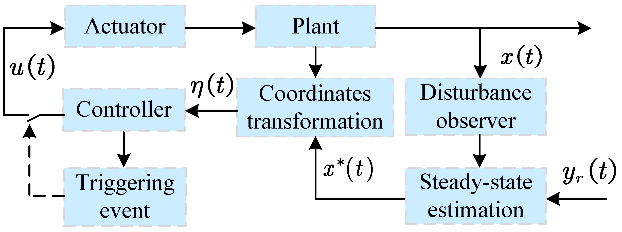
3. Non-Recursive Event-Triggered Control Design Framework

This section presents a step-by-step procedure for constructing an event-triggered controller within a non-recursive framework. For better illustration and comprehension, the entire process is depicted in Figure 1. In this scheme, the communication between the controller and the actuator is determined by the triggering event, thereby reducing the communication load between them.

3.1. Disturbance Observation

Consider the i-th subsystem $x_i=x_{i+1}+f_i\left({\overline{x}}_i\right)+d_i$, by setting $x_i=z_{i,1}$ and $d_i^{\left(j\right)}=z_{i,j+2},j\in {\mathbb{N}}_{0:n-i+1}$, the following extended system can be obtained:

$$\begin{array}{c}\hfill \left\{\begin{array}{c}{\dot{z}}_{i,1}=x_{i+1}+f_i\left({\overline{x}}_i\right)+z_{i,2},\hfill \\ {\dot{z}}_{i,j}=z_{i,j+1},j\in {\mathbb{N}}_{2:n-i+1},\hfill \\ {\dot{z}}_{i,n-i+2}=d_i^{(n-i+1)}.\hfill \end{array}\right.\end{array}$$

(3)

To achieve performance recovery under unknown disturbances, inspired by [24], a practical high-gain disturbance observer can be constructed as follows:

$$\begin{array}{c}\hfill \left\{\begin{array}{c}{\dot{\widehat{z}}}_{i,1}=x_{i+1}+f_i\left({\overline{x}}_i\right)+{\widehat{z}}_{i,2}+h_{i,1}{\ell }_i(z_{i,1}-{\widehat{z}}_{i,1}),\hfill \\ {\dot{\widehat{z}}}_{i,j}={\widehat{z}}_{i,j+1}+h_{i,j}{\ell }_i^j(z_{i,1}-{\widehat{z}}_{i,1}),j\in {\mathbb{N}}_{2:n-i+1},\hfill \\ {\dot{\widehat{z}}}_{i,n-i+2}=h_{i,n-i+2}{\ell }_i^{n-i+2}(z_{i,1}-{\widehat{z}}_{i,1}),\hfill \end{array}\right.\end{array}$$

(4)

where ${\widehat{z}}_{i,1}$, ${\widehat{z}}_{i,2}$, and ${\widehat{z}}_{i,j+1},j\in {\mathbb{N}}_{2:n-i+2}$ correspond to the estimated values of $x_i$, $d_i$, and $d_i^{(j-1)}$, respectively. ${\ell }_i\ge 1$ represents the parameter to be designed, and the observer gains ${[H_{i,j},h_{i,n-i+2}]}^{\top }$ serve as the coefficient matrix for the Hurwitz polynomial $p_1=s^{n-i+2}+h_{i,1}{s}^{n-i+1}+\cdots +h_{i,n-i+1}s+h_{i,n-i+2}$, where $H_{i,j}=[h_{i,1},h_{i,2},\cdots ,h_{i,n-i+1}]$.

Combining (3) and (4), and introducing the transformation $e_{i,j}=(z_{i,j}-{\widehat{z}}_{i,j})/{\ell }_i^{j-1}$, $j\in {\mathbb{N}}_{1:n-i+2}$, the expression for the error dynamics can be calculated as:

$$\begin{array}{c}\hfill \left\{\begin{array}{c}{\dot{e}}_{i,j}={\ell }_i{e}_{i,j+1}-h_{i,j}{\ell }_i{e}_{i,1},j\in {\mathbb{N}}_{1:n-i+1},\hfill \\ {\dot{e}}_{i,n-i+2}=-h_{i,n-i+2}{\ell }_i{e}_{i,1}+d_i^{(n-i+1)}/{\ell }_i^{n-i+1},\hfill \end{array}\right.\end{array}$$

(5)

which can also be rewritten in the following state-space form:

$$\begin{array}{c}\hfill {\dot{e}}_i={\ell }_i{A}_i{e}_i+\Xi \left(d_i^{(n-i+1)}\right)/{\ell }_i^{n-i+1},\end{array}$$

(6)

where $A_i=\left[\begin{array}{cc}-H_{i,j}^{\top }& I_{n-i+1}\\ -h_{i,n-i+2}& 0\end{array}\right]$, $\Xi ={[0,\cdots ,0,1]}^{\top }$, $e_i={[e_{i,1},\cdots ,e_{i,n-i+2}]}^{\top }$.

Clearly, $A_i$ is a Hurwitz matrix, implying the existence of a positive definite and symmetric matrix $Q_i$ satisfying $A_i^{\top }{Q}_i+Q_i{A}_i\le -I$. Then, by constructing the Lyapunov function $W_i\left(e_i\right)=e_i^{\top }{Q}_i{e}_i$ and differentiating along (6), the following relation can be obtained:

$$\begin{array}{cc}\hfill {\dot{W}}_i\left(e_i\right)& \le -l_i{\parallel e_i\parallel }^2+2e_i^{\top }\Xi Q_i{d}_i^{n-i+1}/{\ell }_i^{n-i+1}\hfill \\ \hfill & \le -l_i\parallel e_i{\parallel }^2+2\parallel Q_i\parallel \parallel e_i\parallel \overline{D}\hfill \\ \hfill & \le -({\ell }_i-c_i){\parallel e_i\parallel }^2+{\overline{D}}^2,\hfill \end{array}$$

(7)

where $c_i={\parallel Q_i\parallel }^2$ and $\overline{D}=D/{\ell }^{n-i+1}$.

Hence, a preliminary conclusion can be drawn from (7): by selecting sufficiently large parameters ${\ell }_i,i\in {\mathbb{N}}_{1:n}$ to ensure ${\ell }_i-c_i>0$, it is possible to drive the error system (6) arbitrarily close to zero. In other words, the observer (4) achieves the estimation of disturbances and their corresponding order derivatives.

Remark 3. 

A finite-time disturbance observer based on a higher-order sliding mode (HOSM) method is presented in [24], which achieves finite-time observation for bounded disturbances. The observer (4) offers an alternative approach that does not prioritize observation time, featuring a much simpler gain-tuning mechanism.

3.2. Steady-State Estimations

As stated in [25], the steady-state response of system (1) can be calculated according to the information of tracking signals and external disturbances, as follows:

$$\begin{array}{c}\hfill \left\{\begin{array}{cc}\hfill {\varsigma }_1& =y_r,\hfill \\ \hfill {\varsigma }_i& ={\dot{\varsigma }}_{i-1}-f_{i-1}\left({\overline{\varsigma }}_{i-1}\right)-d_{i-1},i\in {\mathbb{N}}_{2:n+1},\hfill \end{array}\right.\end{array}$$

(8)

by substituting $d_i^{\left(j\right)}$ in (8) with ${\widehat{z}}_{i,j+2}$ for $i\in {\mathbb{N}}_{1:n}$, $j\in {\mathbb{N}}_{0:n-i+1}$, the following set of steady-state estimations of system (1) can be obtained:

$$\begin{array}{c}\hfill x_i^{*}={\varsigma }_i(\widehat{z},{\overline{y}}_r),i\in {\mathbb{N}}_{1:n+1},\end{array}$$

(9)

where ${\overline{y}}_r={[y_r,y_r^{\left(1\right)}\cdots ,y_r^{\left(n\right)}]}^{\top }.$

3.3. Coordinates Transformation

In what follows, introducing an adjustable high gain $L\ge 1$ and defining the coordinate transformation ${\eta }_i=\frac{x_i-x_i^{*}}{L^{i-1}},i\in {\mathbb{N}}_{1:n}$, a stabilizable system can be formulated as:

$$\begin{array}{c}\hfill \left\{\begin{array}{c}{\dot{\eta }}_i=L{\eta }_{i+1}+(f_i\left({\overline{x}}_i\right)-f_i\left({\overline{x}}_i^{*}\right))/L^{i-1}+{\mu }_i/L^{i-1},i\in {\mathbb{N}}_{1:n-1},\hfill \\ {\dot{\eta }}_n=\frac{u-x_{n+1}^{*}}{L^{n-1}}+\left(f_n\left(x\right)-f_n\left(x^{*}\right)\right)/L^{n-1}+{\mu }_n/L^{n-1},\hfill \end{array}\right.\end{array}$$

(10)

where ${\mu }_i=f_i\left({\overline{x}}_i^{*}\right)+x_{i+1}^{*}-{\dot{x}}_i^{*}-\left(f_i\left({\overline{\varsigma }}_i\right)-{\dot{\varsigma }}_i+{\varsigma }_{i+1}\right)$, it is apparent that ${\mu }_i$ is related to the observation error in (4). Thus, there exists a positive and bounded constant E, such that $\underset{i\in {\mathbb{N}}_{1:n}}{sup}\left\{\right|{\mu }_i\left|\right\}\le E$.

3.4. Event-Triggered Controller Design

At this point, the control law can be directly presented without any recursive computations:

$$\begin{array}{cc}\hfill w\left(t\right)& =-L^{n}K\eta +x_{n+1}^{*}-\overline{m}tanh\left(\frac{{\eta }^{\top }PB}{\epsilon L^{n-1}}\right),\hfill \end{array}$$

(11)

the triggering event is defined as:

$$\begin{array}{cc}\hfill u\left(t\right)& =w\left(t_k\right),\forall t\in [t_k,t_{k+1}),k=0,1,2,\cdots ,\hfill \\ \hfill t_{k+1}& =inf\{t>t_k\mid |w\left(t\right)-u\left(t\right)|>m\},t_1=0,\hfill \end{array}$$

(12)

where $\epsilon$, m, $\overline{m}$ are positive constants, and $\overline{m}>m$. $t_k$ is the controller updating time. $K=[k_1,k_2,\cdots ,k_n]$ is the coefficient matrix of the Hurwitz polynomial $p\left(s\right)=s^n+k_n{s}^{n-1}+\cdots +k_{2}s+k_1$. $\eta ={[{\eta }_1,{\eta }_2\cdots {\eta }_n]}^{\top }$. The definitions of matrices B and P will be provided in (14) and (15), respectively.

Remark 4. 

According to the designed trigger event, whenever (12) is satisfied, the time will be marked as $t_{k+1}$ and the control value $u\left(t_{k+1}\right)$ will be applied to the system. During the time $t\in [t_k,t_{k+1})$, the control signal holds as a constant, i.e., $w\left(t_k\right)$. Considering causality, $t_{k+1}^{-}$ is defined as the moment when the event is satisfied and $t_{k+1}$ as the moment of the controller $u\left(t\right)$ update.

Remark 5. 

After implementing a triggering event with a fixed threshold, the last term of $w\left(t\right)$ provides compensatory adjustments for sampling errors. When $m=\overline{m}=0$, controller (11) simplifies to the standard non-recursive controller proposed in [26].

4. Main Result

The main result of this paper can be summarized as the following theorem.

Theorem 1. 

Consider system (1) under Assumptions 1–3. The event-triggered controller (11) with (12) holds the following statements for any initial value:

• All signals in the resulting closed-loop system are bounded and the tracking error will exponentially converge to a set.
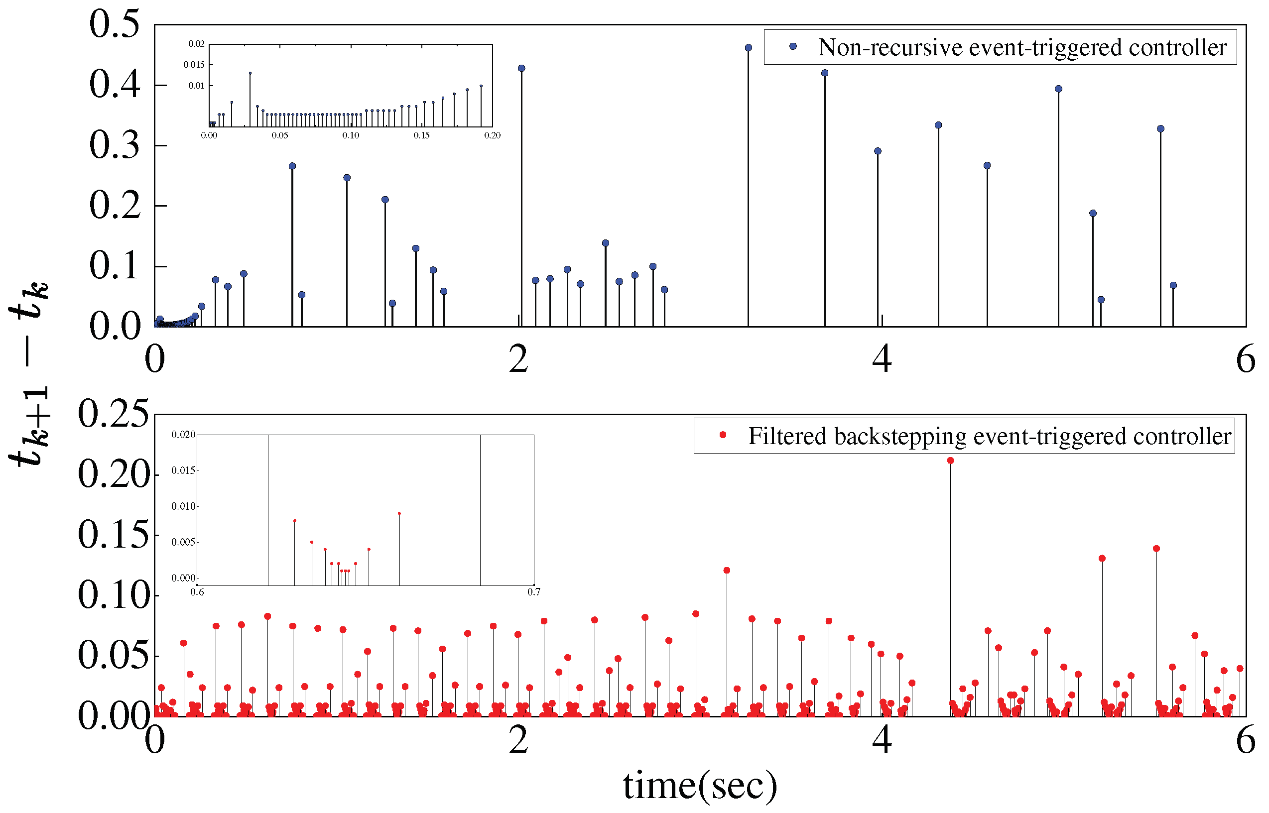
• The inter-execution intervals $t_{k+1}-t_k>0$ indicate the absence of the Zeno phenomenon.

Proof of Theorem 1. 

According to the triggering event (12), for $\forall t\in [t_k,t_{k+1})$, there exists a time-varying parameter $\gamma \left(t\right)$ that satisfies the following conditions:

$$\begin{array}{c}\hfill \left\{\begin{array}{c}\gamma \left(t_k\right)=0,\gamma \left(t_{k+1}^{-}\right)=\pm 1,\left|\gamma \left(t\right)\right|\le 1,\hfill \\ w\left(t\right)=u\left(t\right)+m\gamma \left(t\right).\hfill \end{array}\right.\end{array}$$

(13)

Consequently, by combining (10), (11) and (13), the closed-loop system can be obtained in the following form:

$$\begin{array}{cc}\hfill & \dot{\eta }=LA\eta -B\frac{\overline{m}tanh\left(\frac{{\eta }^{\top }PB}{\epsilon L^{n-1}}\right)+m\gamma \left(t\right)}{L^{n-1}}+F\left(·\right)+\mu ,\hfill \end{array}$$

(14)

where A and B constitute the n-th order controllable matrix pair, $F(·)={[f_1\left(x\right)-f_1\left(x_1^{*}\right),\cdots ,(f_n\left(x\right)-f_n\left(x^{*}\right))/L^{n-1}]}^{\top }$, $\mu ={[{\mu }_1,{\mu }_2/L^1,\cdots ,{\mu }_n/L^{n-1}]}^{\top }$.

Given that A is a Hurwitz matrix, there exists a positive definite matrix $P=P^{\top }$, such that:

$$\begin{array}{c}\hfill A^{\top }P+PA\le -I.\end{array}$$

(15)

Hence, constructing the Lyapunov function $V\left(\eta \right)={\eta }^{\top }P\eta$ and differentiating it along the closed-loop system (14), the following result can be obtained:

$$\begin{array}{cc}\hfill \dot{V}\left(\eta \right)& =L{\eta }^{\top }\left(A^{\top }P+PA\right)\eta +2{\eta }^{\top }PF\left(·\right)+2{\eta }^{\top }P\mu \hfill \\ \hfill & -2{\eta }^{\top }PB\frac{\overline{m}tanh\left(\frac{{\eta }^{\top }PB}{\epsilon L^{n-1}}\right)+m\gamma \left(t\right)}{L^{n-1}}.\hfill \end{array}$$

(16)

Considering the matrix P in (15), it naturally yields that:

$$\begin{array}{c}\hfill L{\eta }^{\top }\left(A^{\top }P+PA\right)\eta \le -L{\parallel \eta \parallel }^2.\end{array}$$

(17)

According to Assumption 1, it can be derived that:

$$\begin{array}{cc}\hfill & \frac{f_i\left({\overline{x}}_i\right)-f_i\left({\overline{x}}_i^{*}\right)}{L^{i-1}}\le \frac{{\sigma }_i}{L^{i-1}}\left(\right|x_1-x_1^{*}|+\cdots +|x_i-x_i^{*}\left|\right)\hfill \\ \hfill & \le {\sigma }_i\left(\right|{\eta }_1|+|{\eta }_2|+\cdots +|{\eta }_i\left|\right)\le {\sigma }_i\sqrt{\eta }\parallel \eta \parallel ,\hfill \end{array}$$

(18)

furthermore, it is easily to conclude that:

$$\begin{array}{c}\hfill 2{\eta }^{\top }PF\left(·\right)\le {2\sigma n\parallel P\parallel \parallel \eta \parallel }^2={\delta }_1{\parallel \eta \parallel }^2,\end{array}$$

(19)

where $\sigma =max\left\{{\sigma }_i\right\}$, ${\delta }_1=2\sigma n\parallel P\parallel$.

With $\underset{i\in {\mathbb{N}}_{1:n}}{sup}\left\{\right|{\mu }_i\left|\right\}\le E$, the following relation can be derived:

$$\begin{array}{c}\hfill 2{\eta }^{\top }P\mu \le {n\parallel P\parallel }^2{\parallel \eta \parallel }^2+E^2={\delta }_2{\parallel \eta \parallel }^2+E^2,\end{array}$$

(20)

where ${\delta }_2=n{\parallel P\parallel }^2$.

Note that, for any $\epsilon >0$ and real number $\rho$, the function $tanh(·)$ satisfies the inequality $0\le \left|\rho \right|-\rho tanh\left(\frac{\rho }{\epsilon }\right)\le 0.2785\epsilon$. Hence, in conjunction with the conditions $\left|\gamma \left(t\right)\right|\le 1$ and $\overline{m}>m$, the final term in (16) can be estimated as:

$$\begin{array}{c}\hfill -2\left[m\gamma \left(t\right)\frac{{\eta }^{\top }PB}{L^{n-1}}+\overline{m}\frac{{\eta }^{\top }PB}{L^{n-1}}tanh\left(\frac{\frac{{\eta }^{\top }PB}{L^{n-1}}}{\epsilon }\right)\right]\le 0.557\epsilon .\end{array}$$

(21)

Finally, combining with (17)–(21), (16) can be rewritten as:

$$\begin{array}{c}\hfill \dot{V}\left(\eta \right)\le -(L-{\delta }_1-{\delta }_2){\parallel \eta \parallel }^2+E^2+0.557\epsilon .\end{array}$$

(22)

Therefore, the gain L can be selected according to the criterion that $L\ge 2({\delta }_1+{\delta }_2)$. Additionally, considering $\parallel \eta \parallel \ge {\lambda }_{max}^{-1}\left(P\right)V\left(\eta \right)$, where ${\lambda }_{max}\left(P\right)$ is the largest eigenvalue of matrix P, the following can be inferred:

$$\begin{array}{c}\hfill \dot{V}\left(\eta \right)\le -\frac{L}{2}{\lambda }_{max}^{-1}\left(P\right)V\left(\eta \right)+E^2+0.557\epsilon .\end{array}$$

(23)

Thus, all signals in the closed-loop system are uniformly bounded, and the tracking error satisfies:

$$\begin{array}{c}\hfill {\lambda }_{min}\left(P\right){\eta }_1^2\le V\left(\eta \right)\le e^{-\alpha }V\left(0\right)+(\Delta /\alpha )(1-e^{-\alpha t}),\end{array}$$

(24)

namely, ${\eta }_1^2$ converges exponentially to a boundary $\Omega$ at a rate of $\alpha$:

$$\begin{array}{c}\hfill \Omega =\{{\eta }_1\mid {\eta }_1^2\le \Delta /\left({\lambda }_{min}\left(P\right)\alpha \right)\},\end{array}$$

(25)

where ${\lambda }_{min}\left(P\right)$ is the smallest eigenvalue of matrix P, $\alpha =\frac{L}{2}{\lambda }_{max}^{-1}\left(P\right)$, $\Delta =E^2+0.557\epsilon$.

Furthermore, for any $t\in [t_k,t_{k+1})$, defining $e_u\left(t\right)=w\left(t\right)-u\left(t\right)$, due to the fact that $\frac{d}{dt}\left|e_u\right|=\frac{d}{dt}{\left(e_u·e_u\right)}^{\frac{1}{2}}\le \left|\dot{w}\right|$ and according to (11), it can be deduced that:

$$\begin{array}{c}\hfill \dot{w}\left(t\right)={\left(-L^{n}K\eta +x_{n+1}^{*}\right)}^{\left(1\right)}-\frac{{\left(\overline{m}{\eta }^{\top }PB\right)}^{\left(1\right)}}{{cosh}^2\left(\frac{{\eta }^{\top }PB}{\epsilon L^{n-1}}\right)}.\end{array}$$

(26)

As previously stated, both $\eta$ and $x_{n+1}$ are differentiable and bounded variables. Therefore, there exists a constant $\kappa >0$ such that $\left|\dot{w}\right|<\kappa$. Additionally, considering $e_u\left(t_k\right)=0$ and $e_u\left(t_{k+1}^{-}\right)=m$, it follows that $t=t_{k+1}-t_k>\frac{m}{\kappa }$, indicating the absence of the Zeno phenomenon. □

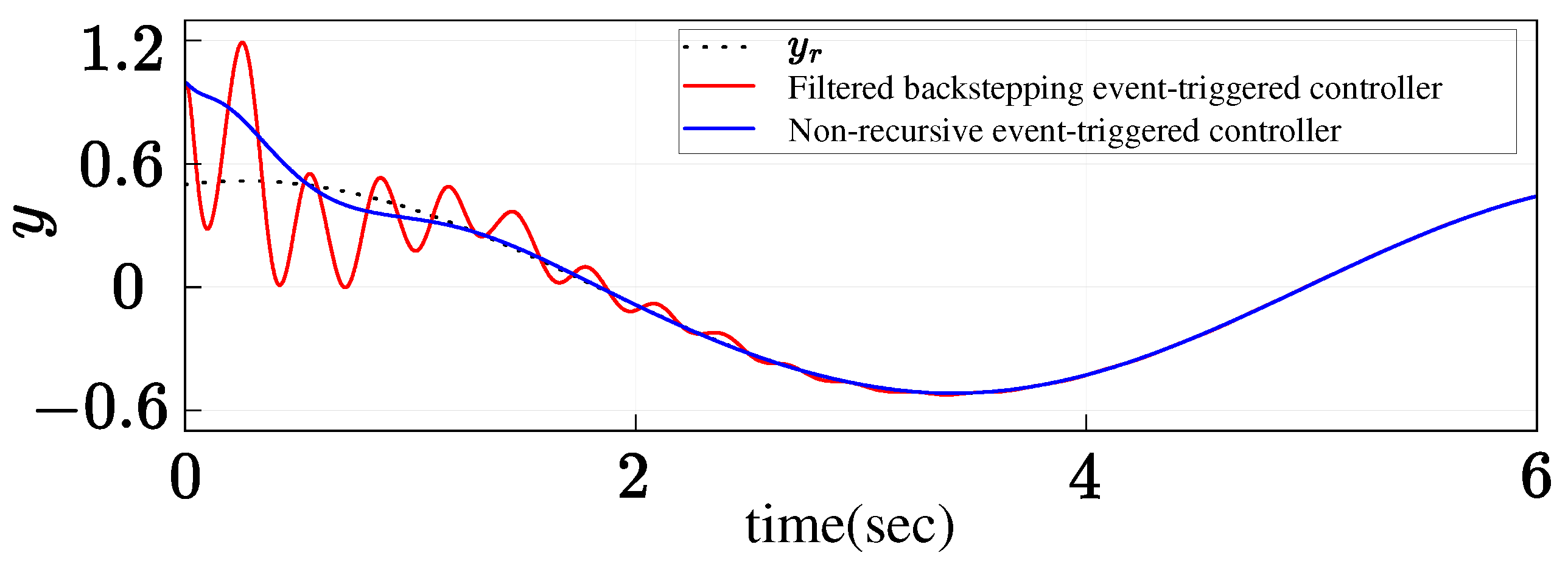
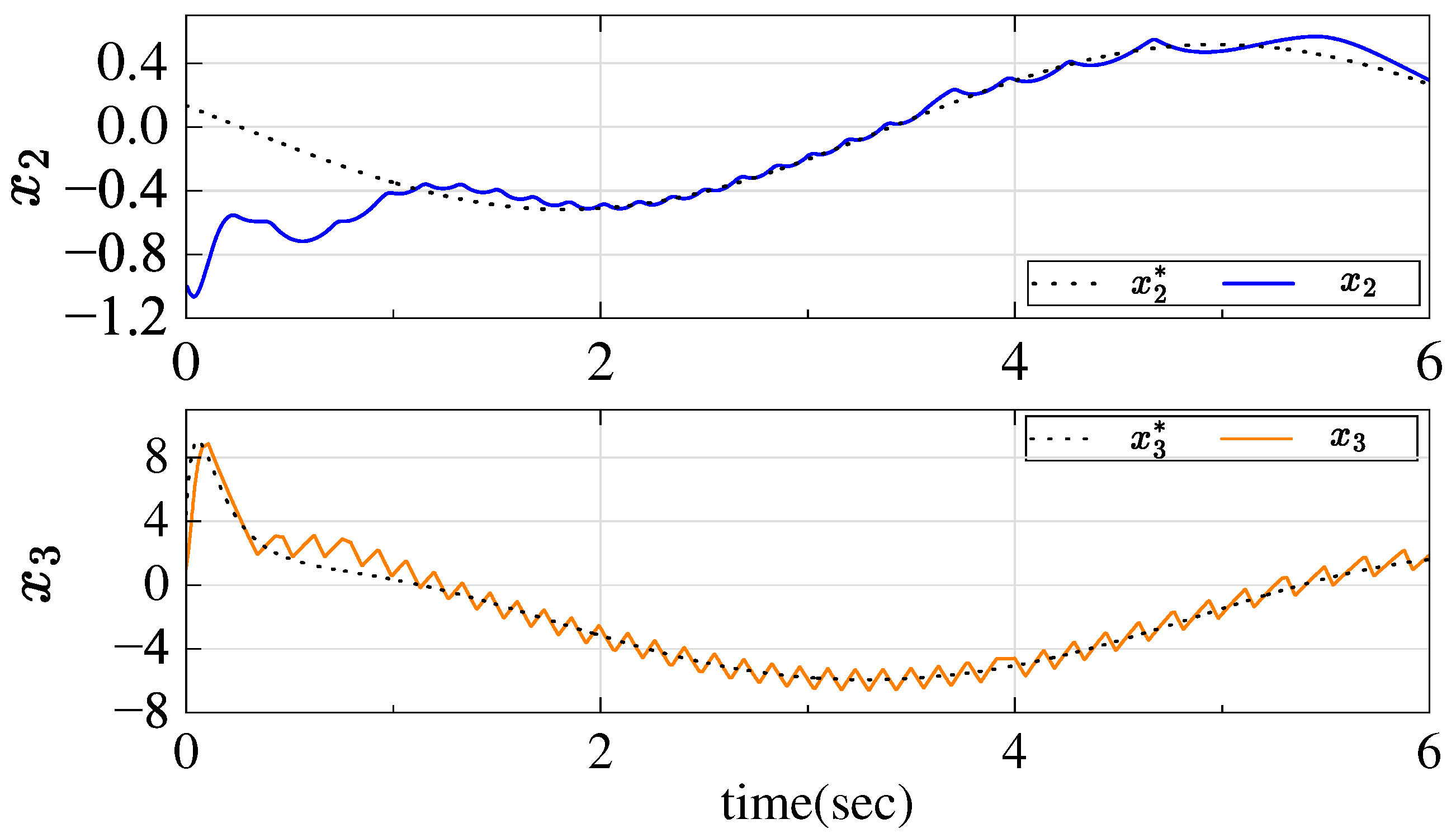
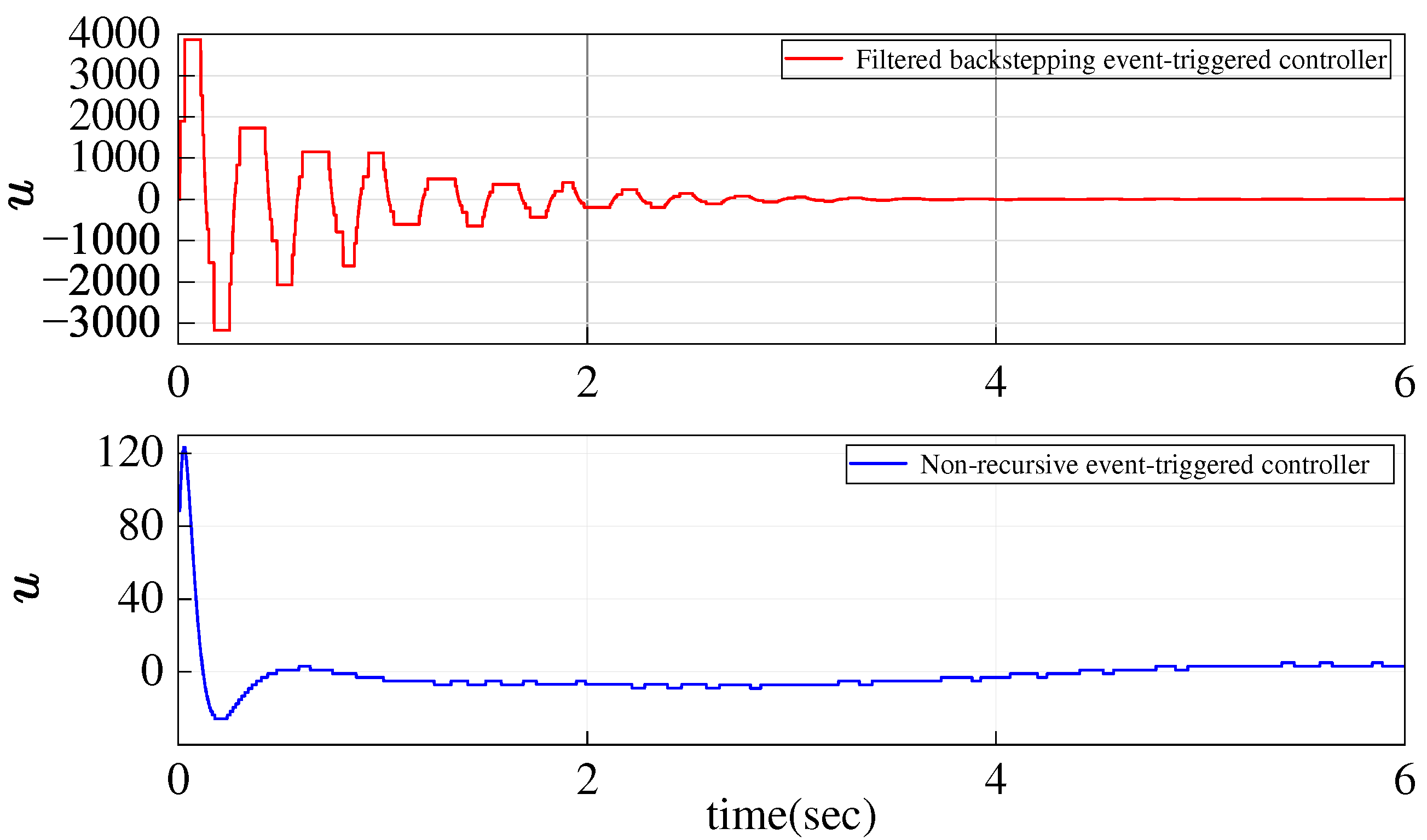
5. Numerical Simulations

A typical single-link robot arm system reported in [27] with parameters selected according to [26] can be represented by the following mathematical model:

$$\begin{array}{c}\hfill \left\{\begin{array}{cc}\hfill {\dot{x}}_1& =x_2,{\dot{x}}_2=x_3-10sin\left(x_1\right)-x_2+d_1,\hfill \\ \hfill {\dot{x}}_3& =u-0.2x_2-x_3+d_2.\hfill \end{array}\right.\end{array}$$

(27)

In the following simulation, the given tracking reference signal is $y_r=sin\left(t\right)+cos(t+\pi /3)$, and the time-varying disturbances are introduced as $d_1=2+0.5cos\left(t\right)$ and $d_2=0.5e^{-t}$, with the initial value $x_0=[1,-1,1]$. According to the proposed non-recursive event-triggered control design framework, the candidate controller can be obtained through the following steps.

Step 1. Disturbance observation: the following disturbance observers are built to estimate $d_1$ and $d_2$ according to (4):

$$\begin{array}{cc}\hfill d_1& \left\{\begin{array}{c}{\dot{\widehat{z}}}_{2,1}=x_3-x_2-10sin\left(x_1\right)+{\widehat{z}}_{2,2}+h_{2,1}{\ell }_2\left(z_{2,1}-{\widehat{z}}_{2,1}\right),\hfill \\ {\dot{\widehat{z}}}_{2,2}={\widehat{z}}_{2,3}+h_{2,2}{{\ell }_2}^2\left(z_{2,1}-{\widehat{z}}_{2,1}\right),\hfill \\ {\dot{\widehat{z}}}_{2,3}=h_{2,3}{{\ell }_2}^3\left(z_{2,1}-{\widehat{z}}_{2,1}\right);\hfill \end{array}\right.\hfill \\ \hfill d_2& \left\{\begin{array}{c}{\dot{\widehat{z}}}_{3,1}=u-0.2x_2-x_3+{\widehat{z}}_{3,2}+h_{3,1}{\ell }_3\left(z_{3,1}-{\widehat{z}}_{3,1}\right),\hfill \\ {\dot{\widehat{z}}}_{3,2}=h_{3,2}{{\ell }_3}^2\left(z_{3,1}-{\widehat{z}}_{3,1}\right).\hfill \end{array}\right.\hfill \end{array}$$

Step 2. Steady-state estimations: based on (8), the estimated steady-state reference signals for system (27) are as follows: $x_1^{*}=y_r$, $x_2^{*}={\dot{y}}_r$, $x_3^{*}={\ddot{y}}_r+{\dot{y}}_r+10sin\left(y_r\right)-{\widehat{z}}_{2,2}$, and $x_4^{*}=y_r^{\left(3\right)}+{\ddot{y}}_r+10cos\left(y_r\right){\dot{y}}_r-{\widehat{z}}_{2,3}+0.2x_2^{*}+x_3^{*}-{\widehat{z}}_{3,2}$.

Step 3. Coordinate transformation: performing a coordinate transformation results in: ${\eta }_1=x_1-x_1^{*}$, ${\eta }_2=(x_2-x_2^{*})/L$ and ${\eta }_3=(x_3-x_3^{*})/L^2$.

Step 4. Controller design: by substituting ${\eta }_1$, ${\eta }_2$, and ${\eta }_3$ into (11), and combining with the triggering event (12), the desired controller can be obtained directly.

For a class of nonlinear systems represented by System (27), with the employment of filters to handle tracking errors, avoiding the direct differentiation of the virtual control signal, and integrating the control signal into the trigger event design, a filter-based backstepping event-triggered control scheme is proposed in [17]. According to this approach, through iterative recursive computations with stability analysis, a series of virtual control signals can be expressed as:

$$\begin{array}{c}\hfill \left\{\begin{array}{cc}\hfill {\alpha }_1& =-k_1{z}_1-{\dot{\widehat{z}}}_1+x_2,\hfill \\ \hfill {\alpha }_2& =-k_2{z}_2-{\dot{\widehat{z}}}_2+x_3-z_1,\hfill \\ \hfill \dot{v}& =-k_v\left(v-w\right)-z_3+\dot{\widehat{w}},\hfill \end{array}\right.\end{array}$$

(28)

where $z_1=x_1-y_r$, $z_i=x_i-{\alpha }_i,i=2,3$ represent the tracking errors; $w=-k_3{z}_3-{\dot{\widehat{z}}}_3+v-z_2$ is an auxiliary variable; ${\dot{\widehat{z}}}_i=-{\varpi }_i\left({\widehat{z}}_i-z_i\right),i\in {\mathbb{N}}_{1:3}$ and $\dot{\widehat{w}}=-{\varpi }_v\left(\widehat{w}-w\right)$ are command filters, where ${\varpi }_i$ and ${\varpi }_v$ represent filter parameters; and ${\alpha }_1,{\alpha }_2,v$ are virtual control signals.

Furthermore, introducing the triggering event and providing the actual control law as follows:

$$\begin{array}{c}\hfill \left\{\begin{array}{cc}\hfill u\left(t\right)& =v\left(t_k\right),t\in [t_k,t_{k+1}),\hfill \\ \hfill t_{{\Delta }_1}& =\inf \{t>t_k||v\left(t\right)-u\left(t\right)|\ge \gamma \left|u\left(t\right)\right|+\sigma \},\hfill \\ \hfill t_{{\Delta }_2}& =t_{max},\hfill \\ \hfill t_{k+1}& =min\{t_{{\Delta }_1},t_{{\Delta }_2}\},\hfill \end{array}\right.\end{array}$$

(29)

where $\gamma$, $\sigma$, and $t_{max}$ are positive parameters to be designed.

To ensure a fair comparison, parameters are selected to guarantee optimal control performance of the closed-loop system under both controllers. For the disturbance observer: $[h_{2,1},h_{2,2},h_{2,3},{\ell }_1]=[12,25,10,3]$, $[h_{3,1},h_{3,2},{\ell }_3]=[20,12,2]$; and for the non-recursive event-triggered controller: $[L,k_1,k_2,k_3]=[3,6,8,8]$, $B={[0,0,1]}^{\top }$, $P=[6,2,4;2,2,4;4,4,2]$, $\epsilon =0.1$. Additionally, for the filtered backstepping event-triggered controller: $[k_1,k_2,k_3,k_v]=[4,2,14,5]$, $\gamma =0.03$, $\sigma =0.5$, ${\varpi }_1={\varpi }_2={\varpi }_3=200$, ${\varpi }_v=15$, $t_{max}=0.5$.

Figure 2 shows the output curves, indicating that both strategies can achieve the tracking of the system output to the reference signal. However, the filtered backstepping event-triggered controller lacks a disturbance observer to estimate and compensate for disturbances in real-time, resulting in the suboptimal dynamic performance of the system, with certain oscillations and overshoot phenomena present. Additionally, it is worth noting that, although [17] employs command filters to handle tracking errors, thus avoiding direct differentiation of virtual control laws and simplifying the controller form to some extent. While comparing (11) with (28), it is evident that the proposed controller primarily relies on the nominal model of the system, fundamentally differing from backstepping-based methods that obtain the controller through repeated recursive computations.

Figure 3 shows the response curves of states $x_2$ and $x_3$ under the proposed controller, indicating that all states in the closed-loop system are bounded and capable of tracking their steady-state signals.

Figure 4 and Figure 5 display the control input and triggering time intervals, respectively. The controller based on the filtered backstepping method evidently requires greater control energy and triggers more frequently within the same time period.

In summary, the simulation results confirm that the proposed controller not only offers a more concise form, but also demonstrates superior effectiveness in both tracking performance and conserving system resources when compared to the event-triggered control strategy based on the filtered backstepping method in [17].

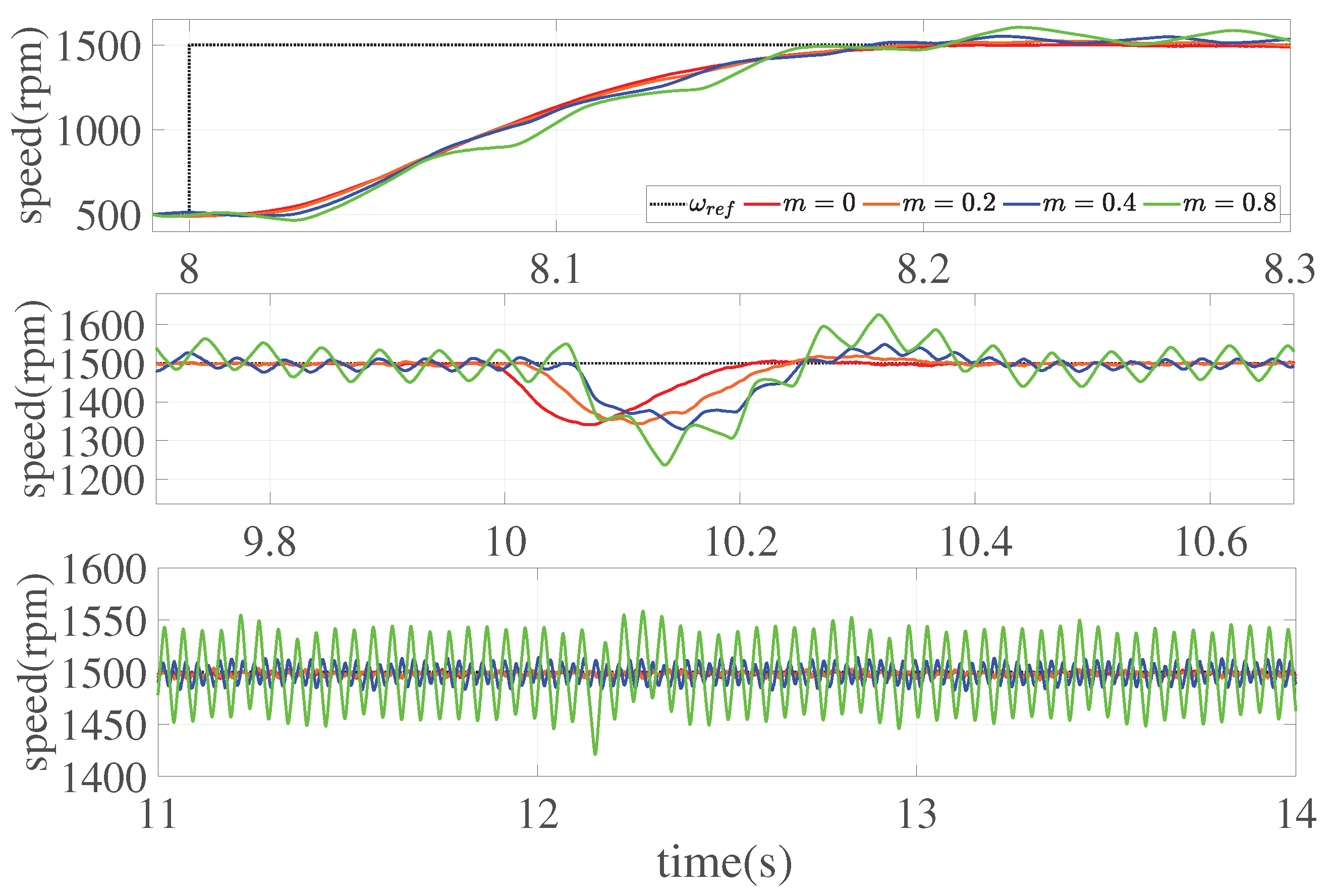
6. Application to Speed Regulation of PMSM

This section takes the speed control of surface-mounted PMSM as an example to validate the effectiveness of the proposed non-recursive event-triggered control strategy. The mathematical model of PMSM in the $d-q$ rotating coordinate system can be articulated as [28]:

$$\begin{array}{c}\hfill \left\{\begin{array}{cc}\hfill \dot{\omega }& =\frac{1}{J}(n_p{\psi }_f{i}_q-B\omega -T_L),\hfill \\ \hfill \dot{i_d}& =\frac{1}{L_s}(-R_s{i}_d+n_p\omega L_s{i}_q+u_d),\hfill \\ \hfill \dot{i_q}& =\frac{1}{L_s}(-R_s{i}_q-n_p\omega L_s{i}_d-n_p{\psi }_f\omega +u_q),\hfill \end{array}\right.\end{array}$$

(30)

where $\omega$ is the mechanical angular velocity, J is the rotor inertia, $n_p$ is the number of pole pairs, ${\psi }_f$ is the rotor flux linkage, B is the viscous frictional coefficient, $T_L$ is the load torque, $R_s$ is the stator resistance, $L_s$ is the stator inductance, and $i_d$, $i_q$, $u_d$ and $u_q$, respectively, denote the stator currents and voltages of the $d$-axis and $q$-axis.

In what follows, with reference speed represented as ${\omega }_{ref}$, defining state variables $x_1={\omega }_{ref}-\omega$, $x_2=\frac{1}{J}(-n_p{\psi }_f{i}_q+B{\omega }_{ref})$ and employing a field-oriented control (FOC) strategy with $i_d=0$, (30) can be rewritten in the form of System (1):

$$\begin{array}{c}\hfill {\dot{x}}_1=x_2-\frac{B}{J}{x}_1+d_1,{\dot{x}}_2=u+f\left(x\right)+d_2,y=x_1,\end{array}$$

(31)

where $d_1=\frac{1}{J}{T}_L$ is the external load viewed as the mismatched disturbance; $d_2$ represents aggregated disturbances encompassing unmodeled dynamics and measurement errors; $f\left(x\right)=\frac{1}{J{L}_s}[-n_p^2{\psi }_f^2{x}_1-R_{s}J{x}_2+(n_p^2{\psi }_f^2+R_{s}B){\omega }_{ref}]$; and $u=-\frac{n_p{\psi }_f}{J{L}_s}{u}_q$ stands for the control input. Then, the original speed control problem is transformed into designing an event-triggered controller, such that the output y of system (31) tracks the reference signal $y_r=0$.

The experiment platform depicted in Figure 6 consists of two Teknic-Motor-M-2310P permanent magnet synchronous motors for testing and load functions. The F28379D module and DRV8305EVM module severed as control core board and control drive board, respectively. The system operates on a 24V DC input and detailed parameters of the PMSM are available in

Table 1. Parameters of the PMSM system.

Symbol	Quantity	Nominal Values
$n_p$	Poles	4
$L_s$	Stator inductance	$2.0\times {10}^{-4}$ H
$R_s$	Stator resistance	$0.36\Omega$
B	Viscous damping	$2.637\times {10}^{-6}\mathrm{N}·\mathrm{m}·\mathrm{s}/\mathrm{rad}$
${\omega }_{max}$	Rated speed	4107 rpm
$I_N$	Rated current	7 A
$V_{dc}$	Bus voltage	24 V
$f_{sw}$	Sampling frequency	20 kHz
${\psi }_f$	Flux linkage	0.0064 Wb
J	Rotor inertia	$7.066\times {10}^{-6}\mathrm{kg}·{\mathrm{m}}^2$

.

Following the proposed non-recursive event-triggered controller design framework, the steady-state estimations are as follows: $x_1^{*}=y_r=0$; $x_2^{*}=-{\widehat{z}}_{1,2}$; $x_3^{*}=-{\widehat{z}}_{1,3}-x_{2,2}-\frac{1}{J{L}_s}(R_{s}J{\widehat{z}}_{2,2}+\left(n_n^2{\psi }_f^2{R}_{s}B\right){\omega }_{ref})$, with the disturbance observation values ${\widehat{z}}_{1,2}$, ${\widehat{z}}_{1,3}$, ${\widehat{z}}_{2,2}$ from observer (4). Similar to steps 3 and 4, the desired event-triggered controller can be obtained. The parameters are chosen as: the disturbance observer: $[h_{1,1},h_{1,2},h_{1,3},{\ell }_1]=[14,5,2,4500]$, $[h_{2,1},h_{2,2},{\ell }_2]=[7,4,3500]$, and the event-triggered controller: $[L,k_1,k_2]=[3,2.5,3]$, $B={[0,1]}^{\top }$, $P=[200,0.5;0.5,200]$, $\epsilon =0.3$. The operating conditions are designed as follows: two cases:

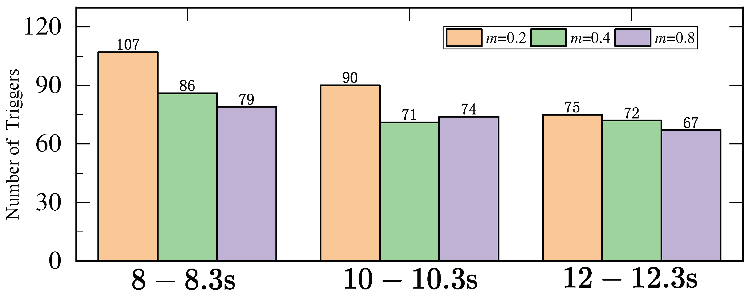
• The motor speed is switched from 500 to 1500 rpm at $t=8$ s;
• A sudden load torque of $T_L=0.5$ Nm is applied at $t=10$ s with the motor speed at 1500 rpm.

Selecting a standard non-recursive controller ($m=0$) and event-triggered controllers with trigger thresholds of $m=0.2$, $0.4$, and $0.8$ for comparison analysis. Figure 7 illustrates the speed response curve, while Figure 8 represents the $q$-axis current curve for the corresponding time interval. Additionally, Figure 9 provides a comparison of trigger occurrences under different triggering thresholds m.

As shown in Figure 7, with the increase in the trigger threshold, the system’s dynamic performance slows down. Furthermore, when an external torque is applied, the system experiences a more pronounced speed drop and slower performance recovery. Additionally, there is a gradual increase in speed oscillation. According to Figure 9, with a sampling frequency of 20 kHz, the introduction of the trigger event achieved the purpose of conserving signal transmission. However, when m increased from 0.4 to 0.8, there was no significant reduction in trigger occurrences, yet the control performance significantly declined.

The experimental results indicate that the proposed algorithm can significantly conserve system resources, while there is no linear relationship between increasing the trigger threshold and conserving system resources. In practical applications, it is only necessary to adjust the trigger threshold m according to specific operating conditions to achieve a trade-off between performance and the conservation of system resources.

7. Conclusions

To address the challenges posed by limited communication and computational resources in practical systems, this paper integrates the event-triggering mechanism with a non-recursive design framework to investigate the tracking control of nonlinear systems with mismatched disturbances. The co-design of the triggering event and controller enables compensation for sampling errors by the controller itself, making it straightforward to strike a balance between control performance and resource conservation. Additionally, simulation and experimental results confirm the simplicity and effectiveness of proposed control strategy.

In the future, the research will continue to explore incorporating state signals into the design of triggering events within a non-recursive framework, thereby reducing the communication load between the sensor and the controller.

References

1. Ding, Z. Global output regulation of uncertain nonlinear systems with exogenous signals. Automatica 2001, 37, 113–119. [Google Scholar] [CrossRef]
2. Chalishajar, D.; Ramkumar, K.; Ravikumar, K.; Anguraj, A.; Anguraj, A. Optimal control of conformable fractional neutral stochastic integrodifferential systems with infinite delay. Results Control Optim. 2023, 13, 100293. [Google Scholar] [CrossRef]
3. Davila, J. Exact tracking using backstepping control design and high-order sliding modes. IEEE Trans. Autom. Control 2013, 58, 2077–2081. [Google Scholar] [CrossRef]
4. Nesic, D.; Teel, A.R.; Carnevale, D. Explicit computation of the sampling period in emulation of controllers for nonlinear sampled-data systems. IEEE Trans. Autom. Control 2009, 53, 619–624. [Google Scholar] [CrossRef]
5. Qian, C.; Du, H. Global output feedback stabilization of a class of nonlinear systems via linear sampled-data control. IEEE Trans. Autom. Control 2012, 57, 2934–2939. [Google Scholar] [CrossRef]
6. Arzen, K. A simple event-based PID controller. Trienn. World Congr. IFAC 1999, 32, 5006–5011. [Google Scholar]
7. Tabuada, P. Event-triggered real-time scheduling of stabilizing control tasks. IEEE Trans. Autom. Control 2007, 52, 1680–1685. [Google Scholar] [CrossRef]
8. Postoyan, R.; Tabuada, P.; Nesic, D.; Anta, A. A framework for the event-triggered stabilization of nonlinear systems. IEEE Trans. Autom. Control 2015, 60, 982–996. [Google Scholar] [CrossRef]
9. Huang, Y.; Liu, Y. Practical tracking via adaptive event-triggered feedback for uncertain nonlinear systems. IEEE Trans. Autom. Control 2019, 64, 3920–3927. [Google Scholar] [CrossRef]
10. Li, H.; Liu, Y.; Huang, Y. Event-triggered controller via adaptive output-feedback for a class of uncertain nonlinear systems. Int. J. Control 2020, 94, 2575–2583. [Google Scholar] [CrossRef]
11. Hua, C.; Li, K.; Guan, X. Decentralized event-triggered control for interconnected time-delay stochastic nonlinear systems using neural networks. Neurocomputing 2018, 272, 270–278. [Google Scholar] [CrossRef]
12. Xing, L.; Wen, C.; Liu, Z.; Su, H.; Cai, J. Event-triggered adaptive control for a class of uncertain nonlinear systems. IEEE Trans. Autom. Control 2016, 64, 2071–2076. [Google Scholar]
13. Li, S.; Yang, J.; Chen, W.; Chen, X. Disturbance Observer-Based Control: Methods and Applications; CRC Press: Boca Raton, FL, USA, 2018. [Google Scholar]
14. Guo, L.; Cao, S. Anti-disturbance control theory for systems with multiple disturbances: A survey. ISA Trans. 2014, 53, 846–849. [Google Scholar] [CrossRef]
15. Zhang, X.; Gu, X.; Yi, Y.; Zhang, T. Event-triggered anti-disturbance tracking control for systems with exogenous disturbances. Chin. Intell. Syst. Conf. 2020, 705, 117–126. [Google Scholar]
16. Li, T.; Wen, C.; Li, S.; Guo, L. Event-triggered tracking control for nonlinear systems subject to time-varying external disturbances. Automatica 2020, 119, 109070. [Google Scholar] [CrossRef]
17. Liu, J.; Yu, J.; Lin, C. Event-triggered and command-filter-based backstepping control for a class of uncertainty nonlinear systems. Control Decis. 2022, 37, 2733–2737. [Google Scholar]
18. Pi, W.; Liu, W. Event-triggered finite-time neural control for uncertain nonlinear systems with unknown disturbances and its application in SVC. Trans. Inst. Meas. Control 2024, 46, 1803–1814. [Google Scholar] [CrossRef]
19. Peng, Z.; Jiang, Y.; Wang, J. Event-triggered dynamic surface control of an underactuated autonomous surface vehicle for target enclosing. IEEE Trans. Ind. Electron. 2020, 68, 3402–3412. [Google Scholar] [CrossRef]
20. Zhang, C.; Yang, J. Nonrecursive Control Design for Nonlinear Systems: Theory and Applications; CRC Press: Roca Boton, FL, USA; London, UK, 2023. [Google Scholar]
21. Xi, Z.; Ding, Z. Global adaptive output regulation of a class of nonlinear systems with nonlinear ecosystems. Automatica 2022, 43, 143–149. [Google Scholar] [CrossRef]
22. Li, M.; Lang, J.; Zhang, C.; Cui, C.; Xu, L. Decentralized composite generalized predictive control strategy for DC microgrids with high PV penetration. Int. J. Robust Nonlinear Control 2022, 32, 7793–7808. [Google Scholar] [CrossRef]
23. Sun, H.; Li, S.; Yang, J.; Guo, L. Non-linear disturbance observer-based back-stepping control for airbreathing hypersonic vehicles with mismatched disturbances. IET Control. Theory Appl. 2014, 8, 1852–1865. [Google Scholar] [CrossRef]
24. Zhang, C.; Yang, J.; Yan, Y.; Fridman, L.; Li, S. Semiglobal finite-time trajectory tracking realization for disturbed nonlinear systems via higher-order sliding modes. IEEE Trans. Autom. Control 2020, 65, 2185–2191. [Google Scholar] [CrossRef]
25. Isidori, A.; Byrnes, C. Output regulation of nonlinear systems. IEEE Trans. Autom. Control 1990, 35, 131–140. [Google Scholar] [CrossRef]
26. Dong, X.; Zhang, C. Nonrecursive robust/adaptive integrated control design framework for nonlinear systems with mismatched disturbances. Control. Theory Appl. 2022, 39, 1641–1650. [Google Scholar]
27. Ho, H.; Wong, Y.; Rad, A. Adaptive fuzzy approach for a class of uncertain nonlinear systems in strict-feedback form. ISA Trans. 2008, 47, 286–299. [Google Scholar] [CrossRef]
28. Dai, C.; Guo, T.; Yang, J.; Li, S. A disturbance observer-based current-constrained controller for speed regulation of PMSM systems subject to unmatched disturbances. IEEE Trans. Ind. 2020, 68, 767–775. [Google Scholar] [CrossRef]
Figure 1. Non-recursive event-triggered control schematic.
Mathematics 12 01716 g001
Figure 2. Response curves of output signals.
Mathematics 12 01716 g002
Figure 3. Response curves of x 2 , x 3 under proposed controller.
Mathematics 12 01716 g003
Figure 4. Response curves of control input.
Mathematics 12 01716 g004
Figure 5. Time interval of triggering event.
Mathematics 12 01716 g005
Figure 6. The experimental platform of PMSM.
Mathematics 12 01716 g006
Figure 7. Speed tracking response curves.
Mathematics 12 01716 g007
Figure 8. The q -axis current response curves.
Mathematics 12 01716 g008
Figure 9. Trigger times under different m.
Mathematics 12 01716 g009