Direct Yaw Moment Control for Distributed Drive Electric Vehicles Based on Hierarchical Optimization Control Framework

Abstract

Direct yaw moment control (DYC) can effectively improve the yaw stability of four-wheel distributed drive electric vehicles (4W-DDEVs) under extreme conditions, which has become an indispensable part of active safety control for 4W-DDEVs. This study proposes a novel hierarchical DYC architecture for 4W-DDEVs to enhance vehicle stability during ever-changing road conditions. Firstly, a vehicle dynamics model is established, including a two-degree-of-freedom (2DOF) vehicle model for calculating the desired yaw rate and sideslip angle as the control target of the upper layer controller, a DDEV model composed of a seven-degree-of-freedom (7DOF) vehicle model, a tire model, a motor model and a driver model. Secondly, a hierarchical DYC is designed combining the upper layer yaw moment calculation and low layer torque distribution. Specifically, based on Matlab/Simulink, improved linear quadratic regulator (LQR) with weight matrix optimization based on inertia weight cosine-adjustment particle swarm optimization (IWCPSO) is employed to compute the required additional yaw moment in the upper-layer controller, while quadratic programming (QP) is used to allocate four motors’ torque with the optimization objective of minimizing the tire utilization rate. Finally, a comparative test with double-lane-change and sinusoidal conditions under a low and high adhesion road surface is conducted on Carsim and Matlab/Simulink joint simulation platform. With IWCPSO-LQR under double-lane-change (DLC) condition on a low adhesion road surface, the yaw rate and sideslip angle of the DDEV exhibits improvements of 95.2%, 96.8% in the integral sum of errors, 94.9%, 95.1% in the root mean squared error, and 78.8%, 98.5% in the peak value compared to those without control. Simulation results indicate the proposed hierarchical control method has a remarkable control effect on the yaw rate and sideslip angle, which effectively strengthens the driving stability of 4W-DDEVs.

1. Introduction

Electrification, intelligence and networking have become a consensus for the future development trend of the global automotive industry. Electric vehicles contribute to reducing environmental pollution and achieve carbon peaking and carbon neutrality goals. Four-wheel distributed drive electric vehicles (4W-DDEVs) adopt a controllable and independent drive motor mounted directly in or near the driving wheel, which has the advantages of quick response, high transmission efficiency, precise control and compact structure [1,2,3]. Thus, 4W-DDEVs are considered as one of the best carriers for vehicle dynamics control technology and have attracted significant attention. However, the larger mass of hub motors will increase the unsprung mass of 4W-DDEVs, potentially resulting in reduced lateral stability and increased complexity of control. Therefore, yaw stability control has become a research focus for 4W-DDEVs. Based on characteristics of 4W-DDEVs, a widely used stability control method is direct yaw moment control (DYC). By generating an additional yaw moment to reduce the vehicle’s yaw rate and sideslip angle, DYC enhances vehicle safety; consequently, the purpose of DYC is to generate the optimal yaw moment [4,5].

The control architecture of DYC can be classified into two groups: centralized control and hierarchical control. The centralized control architecture is generally achieved via a centralized controller sending control instructions to corresponding actuators, and it can also improve the stability control effect by adding various control objectives and constraints [6]. Nevertheless, the complex relationship between multiple control variables may increase the computational time for this kind of control architecture; thus, the real-time performance of the centralized control architecture will become poor [7]. The hierarchical control architecture generally consists of two layers, whereby the upper layer calculates the target additional yaw torque required to maintain the stable operation of the vehicle and the lower layer reasonably distributes the calculated additional yaw torque to each driving wheel [8,9]. Due to the good real-time performance of the hierarchical control architecture provided by decreasing the number of control variables, it has been commonly seen in the field of DYC for 4W-DDEVs [10].

The research on hierarchical DYC mainly concentrates on two aspects: (1) how to determine if the vehicle is unstable in the upper layer; (2) how to accurately allocate the desired torque to four driving motors in the lower layer [11]. For the upper layer, there are currently two main methods to determine if the vehicle is unstable. The first method is to obtain the ideal yaw rate and sideslip angle with a vehicle dynamics model and use them as the ideal variation for tracking control. The second one is to establish the phase plane of the yaw rate and the sideslip angle [12,13]. Although the phase plane method can provide an accurate vehicle stability zone, its real-time performance is very poor. Therefore, the first method is widely used in the upper layer controller of DYC. After the desired yaw rate and sideslip angle are determined, various typical control algorithms are adopted to track the ideal value required for maintaining the vehicle’s stability, including fuzzy control, sliding mode control (SMC), linear quadratic regulator (LQR) and model predictive control (MPC). Liu et al. [14] proposed fuzzy control for DYC, but the design and debug of the fuzzy rule is obtained based on engineering experience. Zhang et al. [15] and Ma et al. [16] presented a SMC strategy with the yaw rate and sideslip angle as control parameters to improve vehicle stability in extreme conditions. However, when the state trajectory gets to the sliding mode surface, it will generate chattering and deteriorate the control effect of the vehicle’s yaw stability. Cao et al. [17] and Lin et al. [18] designed a direct-yaw-moment controller using a LQR algorithm, which has small a steady-state error and good robustness, improving the vehicle handling stability. Nevertheless, further optimization of the weight coefficient should be conducted to improve the control performance of LQR. Zhang et al. [19] and Oh et al. [20] employed MPC to solve the optimal additional yaw moment for following the ideal yaw rate and sideslip. Wu et al. [21] adopted adaptive algorithms to adjust the key time-domain parameters of MPC. Altork et al. [22] and Wang et al. [23] developed robust H∞ state-feedback controllers for yaw stability control that require high-level modeling of the system.

As for torque distribution in the lower layer controller, two kinds of control methods are widely used to allocate the torques: (1) non-optimization methods containing axle load ratio allocation and PID; (2) optimization methods comprising quadratic programming (QP) and least squares. Liao et al. [24] allocated wheel torque according to the axle load ratio, improving the stability margin of the wheels corresponding to lower axle loads. The adaptability of non-optimization allocation methods is weak, especially on a high curvature or low adhesion road, so optimization methods have attracted more attention. Shi et al. [25] proposed a torque optimization allocation based on sequential quadratic programming, whose optimization goal was to minimize tire adhesion utilization. Song et al. [26] and Hang et al. [27] aimed to minimize the longitudinal force of tire and increase the stability margin and solved the torque optimization allocation problem based on the least squares method, which increased computational efficiency. Guo et al. [28] proposed an allocation method based on the Karush–Kuhn–Tucker (KKT) condition with a relatively complex calculation flow.

Based on the above analysis, in order to develop a DYC system with high real-time and good optimization performance, through an improved LQR with weight coefficient optimization and the QP torque allocation method, a hierarchical optimization control framework is employed to study DYC of 4W-DDEVs.

Major contributions of this paper are listed as follows:

(1) A novel hierarchical control framework consisting of two layers is presented to enhance the yaw stability of 4W-DDEVs. An additional yaw moment is acquired using LQR with weight coefficient optimization on the basis of inertia weight cosine-adjustment particle swarm optimization (IWCPSO) in the upper layer controller, and the torque optimization distribution among four wheels is calculated using QP aiming at the minimum tire utilization in the lower layer controller.

(2) Three performance metrics are proposed to quantitatively assess the control performance of the proposed method. The effectiveness and robustness of the hierarchical control framework are fully validated through simulation tests for different maneuver scenarios under low and high adhesion roads.

The following sections of this paper are organized as below. Section 2 presents the system modeling, including a two-degree-of-freedom (2-DOF) reference model, a seven-degree-of-freedom (7-DOF) full vehicle dynamics model, a tire model, a motor model and a closed-loop driver model. Section 3 illustrates the design of the hierarchical controller for yaw stability, involving design of the upper LQR controller, optimization of the Q matrix weight coefficient of LQR and design of the lower optimal torque distribution method. Moreover, the effectiveness of the proposed hierarchical control scheme under two extreme conditions is verified via Carsim-Simulink co-simulation experiments in Section 4. Finally, the conclusions and work to be done in the future are summarized in Section 5.

2. Vehicle Dynamics Model

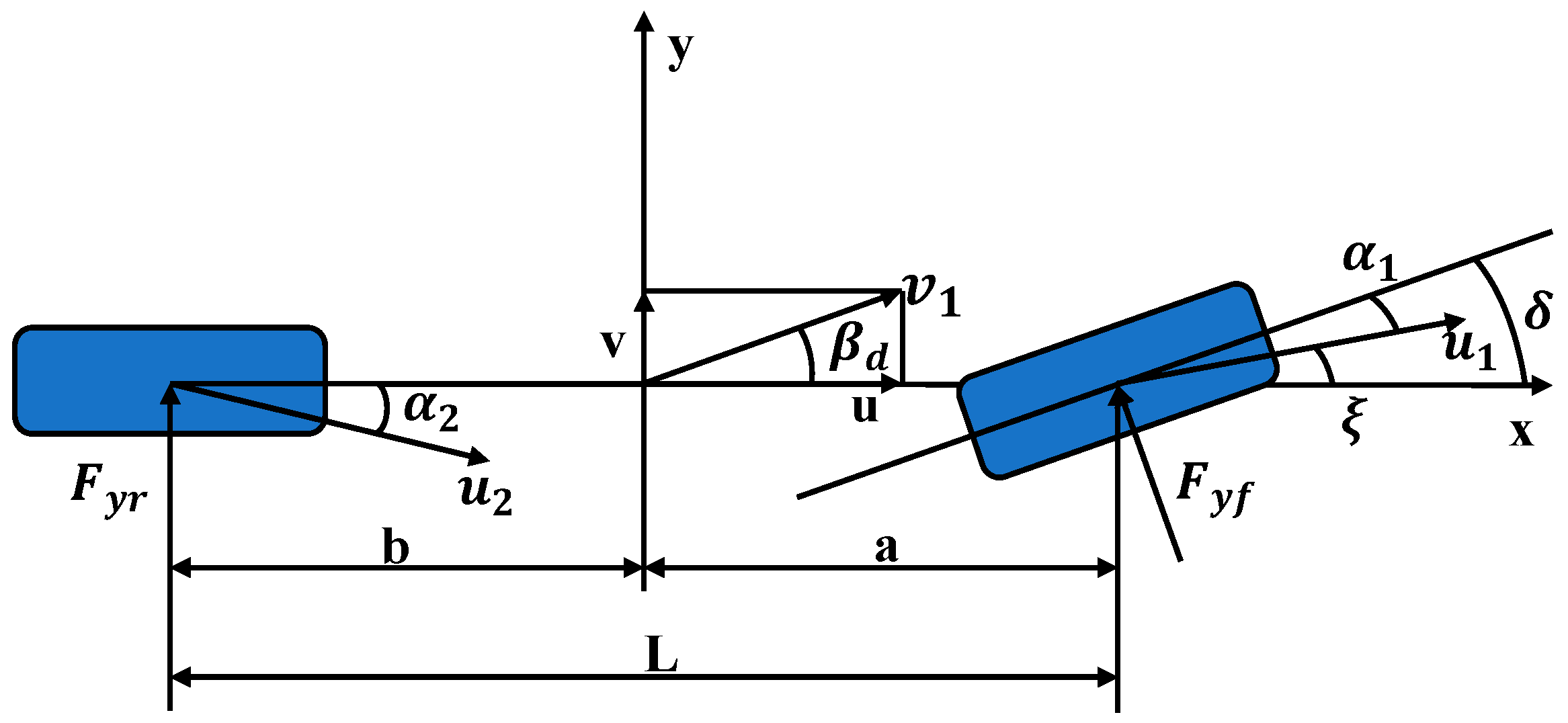
2.1. 2-DOF Reference Model

In this section, a linear 2-DOF vehicle model is used to compute the ideal yaw rate and ideal sideslip angle, which can provide a precise reference value for the subsequent upper controller. A 2-DOF reference model is shown in Figure 1 [29].

The differential equation of the 2-DOF reference model is:

$$\left\{\begin{array}{l}(k_1+k_2){\beta }_d+\frac{1}{u}(a{k}_1-b{k}_2){\omega }_d-k_1\delta =m({\dot{\beta }}_d+{\omega }_d)u\\ (a{k}_1-b{k}_2){\beta }_d+\frac{1}{u}(a^2{k}_1+b^2{k}_2){\omega }_d-a{k}_1\delta =I_z{\dot{\omega }}_d\end{array}\right.$$

(1)

where ${\omega }_d$ is the desired vehicle yaw rate; ${\beta }_d$ is the desired vehicle sideslip angle; $\delta$ is the front wheel steering angle; $I_z$ is the vehicle rotational inertia around the z-axis; $k_1$ and $k_2$ are the cornering stiffness of front and rear tires, respectively; m indicates the vehicle mass; u is the longitudinal vehicle speed; a and b represent the distances from the front and rear axles to the vehicle center of gravity, respectively.

The state space equation of the 2-DOF reference model can be expressed as below:

$$\left[\begin{array}{l}{\dot{\beta }}_d\\ {\dot{\omega }}_d\end{array}\right]=A\left[\begin{array}{l}{\beta }_d\\ {\omega }_d\end{array}\right]+W\delta$$

(2)

where

$$\begin{array}{cc}A=\left[\begin{array}{c}\begin{array}{cc}\frac{k_1+k_2}{mu}& \frac{a{k}_1-b{k}_2}{m{u}^2}-1\end{array}\\ \begin{array}{cc}\frac{a{k}_1-b{k}_2}{I_z}& \frac{a^2{k}_1+b^2{k}_2}{I_{z}u}\end{array}\end{array}\right],& W=\left[\begin{array}{l}-\frac{k_1}{mu}\\ -\frac{a{k}_1}{I_z}\end{array}\right]\end{array}$$

In the steady state of the vehicle, the motion state meets the following conditions: $\dot{\beta }=0, {\dot{\omega }}_r=0$. Based on the 2-DOF reference model, the desired yaw rate and sideslip angle can be obtained. To effectively maintain the consistency of the vehicle driving direction, the sideslip angle is expected to be as small as possible. Hence, the desired yaw rate and sideslip angle are defined in Equation (3) and (4):

$${\omega }_d=\frac{u/L}{1+K{u}^2}\delta$$

(3)

$${\beta }_d=0$$

(4)

where L is the wheel base; K denotes the stability factor, which is defined as follows:

$$K=\frac{m}{L^2}(\frac{a}{k_2}-\frac{b}{k_1})$$

(5)

Considering the nonlinear characteristics of tires, the desired yaw rate is restricted by the road adhesion coefficient. According to the relevant reference, the limit value of the desired yaw rate is expressed in Equation (6):

$$\left|{\omega }_d\right|\le \left|\frac{0.85\mu g}{u}\right|$$

(6)

where $\mu$ is the road adhesion coefficient and $g$ is the acceleration of gravity.

To sum up, reference values for the ideal yaw rate and sideslip angle calculated from the 2-DOF reference model are denoted as follows:

$$\left\{\begin{array}{l}{\omega }_d=min\left\{\left|\frac{0.85\mu g}{u}\right|,\left|\frac{u/L}{1+K{u}^2}\delta \right|\right\}sgn(\delta )\\ {\beta }_d=0\end{array}\right.$$

(7)

2.2. Full Vehicle Model

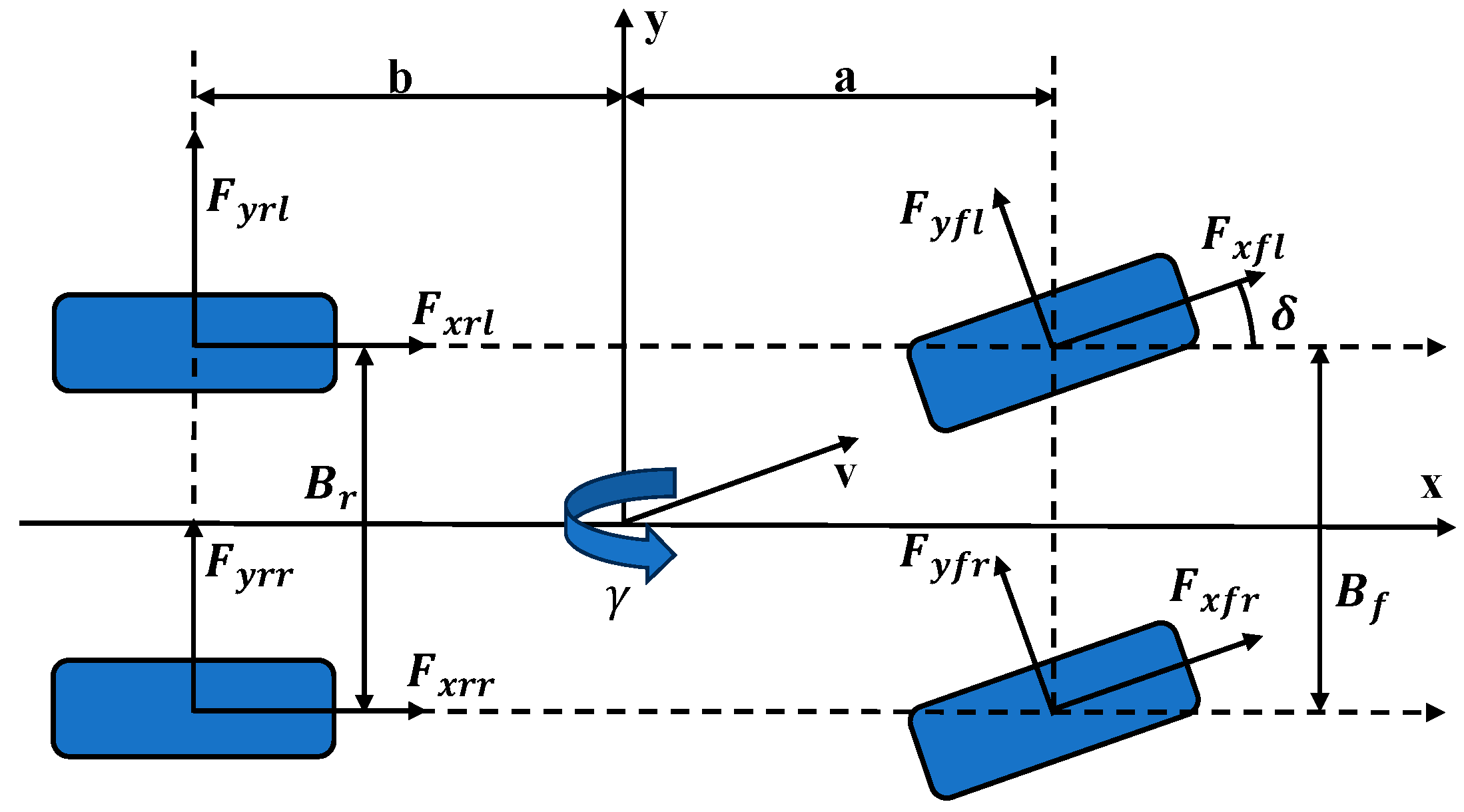
2.2.1. 7-DOF Vehicle Model

Ignoring the vertical and pitch motions, a nonlinear 7-DOF vehicle model is presented to design the upper yaw moment controller, as depicted in Figure 2 [30].

The differential equation of the 7-DOF vehicle model is as follows:

$$\left\{\begin{array}{l}{\displaystyle \sum F_{\mathrm{x}}}=\left(F_{\mathrm{xfl}}+F_{\mathrm{xfr}}\right)cos\delta -\left(F_{\mathrm{yfl}}+F_{\mathrm{yfr}}\right)sin\delta +F_{\mathrm{xfl}}+F_{\mathrm{xrr}}\hfill \\ {\displaystyle \sum F_{\mathrm{y}}}=\left(F_{\mathrm{yfl}}+F_{\mathrm{yfr}}\right)cos\delta +\left(F_{\mathrm{xfl}}+F_{\mathrm{xfr}}\right)sin\delta +F_{\mathrm{yfl}}+F_{\mathrm{yrr}}\hfill \\ M_{\mathrm{z}}=\frac{1}{2}·\frac{B_f+B_r}{2}\left[\left(F_{\mathrm{xfr}}-F_{\mathrm{xfl}}\right)cos\delta +\left(F_{\mathrm{yfl}}-F_{\mathrm{yfr}}\right)sin\delta -F_{\mathrm{xrl}}+F_{\mathrm{xrr}}\right]\hfill \\ \hspace{1em}+a\left[\left(F_{\mathrm{yfl}}+F_{\mathrm{yfr}}\right)cos\delta +\left(F_{\mathrm{xfl}}+F_{\mathrm{xfr}}\right)sin\delta \right]-b\left(F_{\mathrm{yrl}}+F_{\mathrm{yrr}}\right)\hfill \end{array}\right.$$

(8)

where $F_{\mathrm{xi}}$ and $F_{yi}$ are the longitudinal force and lateral force of each tire, respectively $\left(i=fl,fr,rl,rr\right)$; $B_f$ and $B_r$ are the front and rear track, respectively; $M_z$ is the yaw moment.

2.2.2. Tire Model

As one of the important components of the vehicle model, the tire model reflects the nonlinear characteristics of the ground force under different conditions and vehicle states. Hence, it is essential to establish a high-precision tire model for the study of the vehicle’s yaw stability. Due to its ease of use and high accuracy, a widely used semiempirical formula tire model called magic formula (MF) is employed. The universal expression of the MF model is shown as below [31]:

$$F(x)=Dsin\{Carctan[Bx-E(Bx-arctan(Bx))]\}$$

(9)

where $F(x)$ is the output of MF, either the longitudinal force or lateral force; $x$ represents the tire longitudinal slip angle or slip ratio; $B$, $C$, $D$, $E$ denotes the curve correction factors of the MF model, which are the stiffness factor, curve shape factor, peak factor and curvature factor, respectively.

2.2.3. Motor Model

The power to drive 4W-DDEVs comes from four independently controlled motors. Considering the fast transient response characteristic of the motor, the motor model is simplified to the form of a second-order transfer function [32,33]:

$$G(s)=\frac{T_m}{T_m^{*}}=\frac{1}{2{\xi }^2{s}^2+2\xi s+1}$$

(10)

where $T_m^{*}$ is the target output torque of the motor; $T_m$ is the actual output torque of the motor; $\xi$ represents the damping ratio related to the characteristics of the motor, $\xi =0.05$.

2.3. Driver Model

In order to track the target vehicle speed, a driver model is also designed. The driver model is a longitudinal speed tracking controller in essence. Proportional-integral-derivative (PID) control is adopted to make the speed error between the desired vehicle speed and actual vehicle speed close to zero, as well as to obtain the longitudinal torque required by the vehicle.

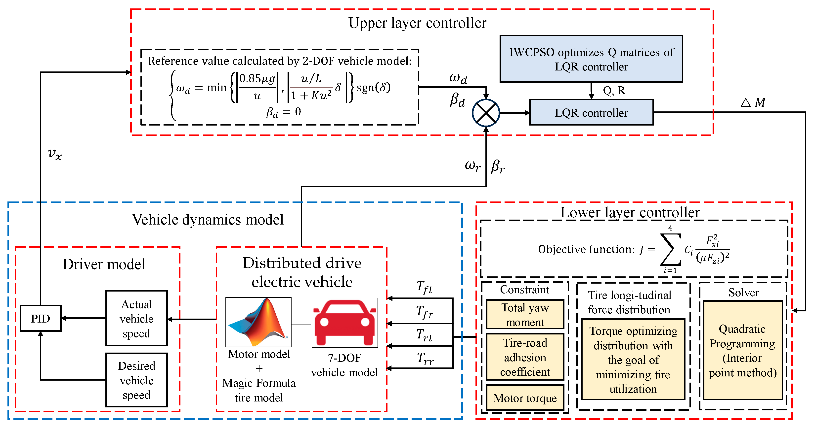
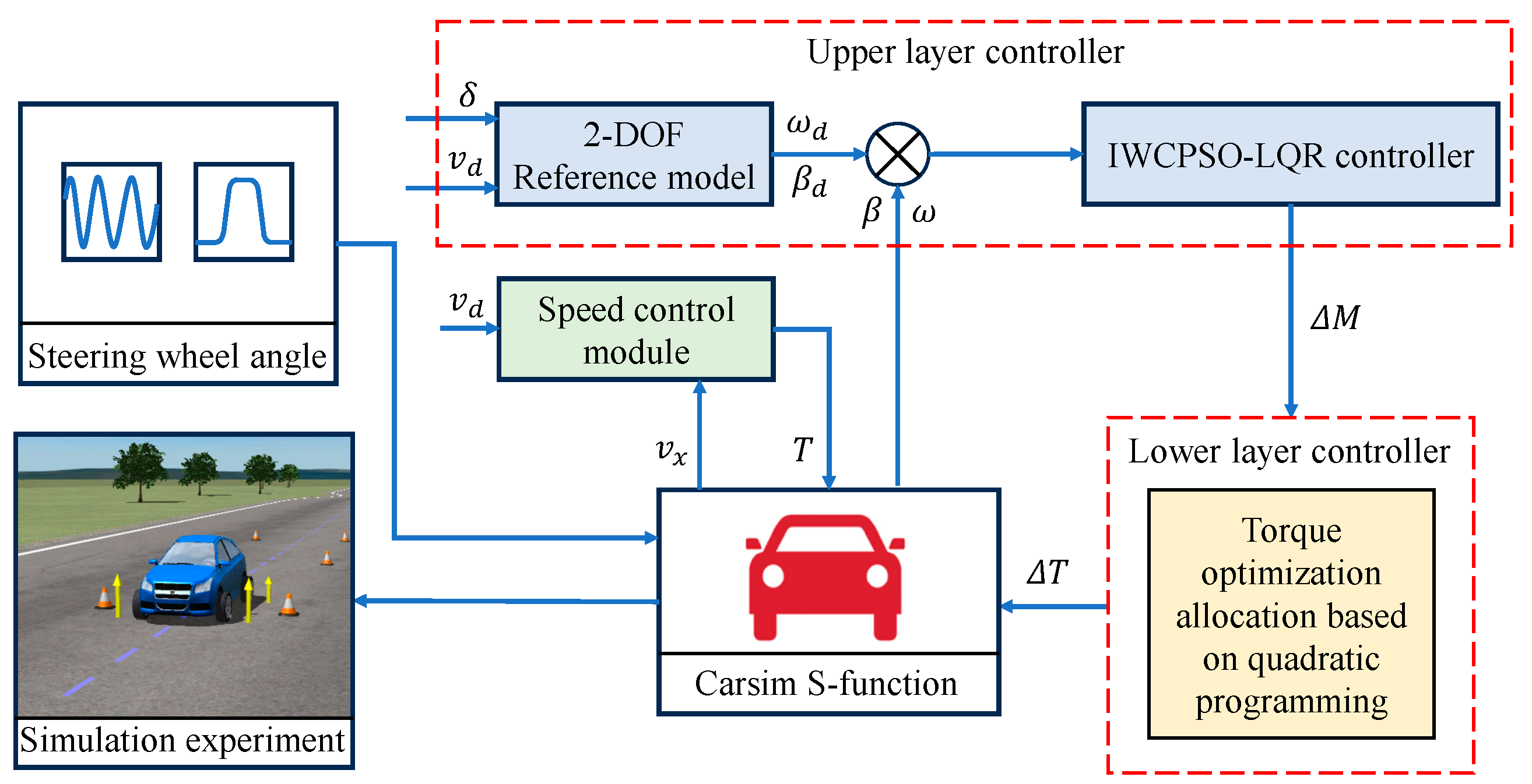
3. Design of Hierarchical Controller for Yaw Stability

The hierarchical control framework of the DYC system studied in this paper is shown in Figure 3.

3.1. Upper Layer Controller Based on IWCPSO-LQR Algorithm

3.1.1. Conventional LQR Controller

The vehicle’s ideal condition determined via the desired vehicle model is as below:

$$\left[\begin{array}{l}0\\ 0\end{array}\right]=A\left[\begin{array}{l}{\beta }_d\\ {\omega }_d\end{array}\right]+W\delta$$

(11)

The 7-DOF vehicle dynamics model with the additional yaw moment is:

$$\left[\begin{array}{l}{\dot{\beta }}_r\\ {\dot{\omega }}_r\end{array}\right]=A\left[\begin{array}{l}{\beta }_r\\ {\omega }_r\end{array}\right]+B\Delta M+W\delta$$

(12)

where ${\beta }_r$ and ${\omega }_r$ represent the actual values of the sideslip angle and yaw rate; $B={\left[\begin{array}{cc}0,& 1/I_z\end{array}\right]}^T$; $\Delta M$ is the additional yaw moment.

The error between the 7-DOF vehicle model and the desired vehicle model is taken as the input variable of the LQR controller. Then, the Riccati equation is computed to acquire the ideal yaw moment that keeps the vehicle’s handling stability. By subtracting Equation (11) from Equation (12), the error state space equations for the sideslip angle and yaw rate can be obtained:

$$\left[\begin{array}{l}\Delta \dot{\beta }\\ \Delta {\dot{\omega }}_r\end{array}\right]=\left[\begin{array}{c}\begin{array}{cc}\frac{k_1+k_2}{mu}& \frac{a{k}_1-b{k}_2}{m{u}^2}-1\end{array}\\ \begin{array}{cc}\frac{a{k}_1-b{k}_2}{I_z}& \frac{a^2{k}_1+b^2{k}_2}{I_{z}u}\end{array}\end{array}\right]·\left[\begin{array}{c}\Delta \beta \\ \Delta {\omega }_r\end{array}\right]+\left[\begin{array}{c}0\\ -\frac{1}{I_z}\end{array}\right]\Delta M$$

(13)

The state variables and input variable are defined as follows:

$$\begin{array}{cc}X={\left[\begin{array}{cc}\Delta \beta ,& \Delta {\omega }_r\end{array}\right]}^T,& U=\Delta M\end{array}$$

Accordingly, the error state space equation for the sideslip angle and yaw rate is written as:

$$\dot{X}=AX+BU$$

(14)

The objective function of the system is described below:

$$J={\displaystyle {\int }_0^{\infty }(X^{T}QX+U^{T}RU)}dt$$

(15)

where Q and R are both weight coefficient matrixes; Q and R are illustrated as follows:

$$\left\{\begin{array}{l}Q=\left[\begin{array}{cc}{q}_1& 0\\ 0& q_2\end{array}\right]\\ R=[r]\end{array}\right.$$

(16)

where $q_1$ and $q_2$ are the weights of the state variables, indicating the importance to the error of the sideslip angle and yaw rate; $r$ is the weight of the input variable, suggesting the constraint on the ideal yaw moment that retains the vehicle’s handling stability.

The optimal feedback matrix is calculated using the Riccati equation, which is expressed as $K=[\begin{array}{cc}{k}_1,& k_2\end{array}]$:

$$\Delta M=-Kx(t)=-k_1\Delta \beta (t)-k_2\Delta {\omega }_r(t)$$

(17)

The optimal control gain matrix can be denoted as:

$$K=R^{-1}{B}^{T}P$$

(18)

where P is the solution of the Riccati equation, which is expressed as below:

$$A^{T}P+PA-PB{R}^{-1}{B}^{T}P+Q=0$$

(19)

Therefore, the solution of the optimal control is as follows:

$$U^{*}=-KX$$

(20)

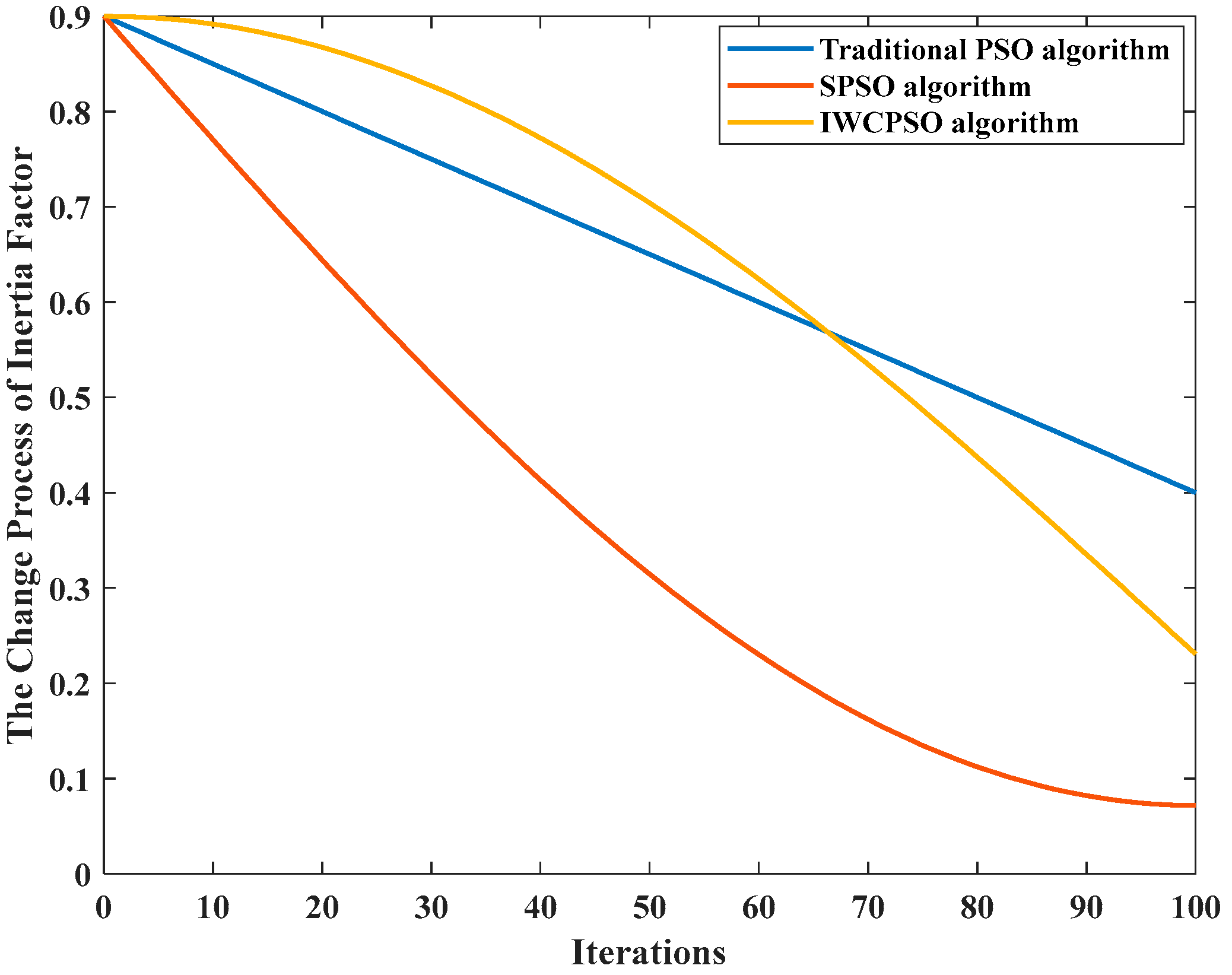
3.1.2. IWCPSO-LQR Controller

The effectiveness of the LQR controller is determined by parameters in weight coefficients matrices Q and R. In the DYC system, R is a first-order square matrix, which is convenient for manual debugging, while Q is a second-order square matrix, where it is difficult to determine the optimal weight coefficient according to engineering experience. Therefore, this section introduces an improved particle swarm optimization (PSO) algorithm to adjust the coefficients $q_1$ and $q_2$ in matrix Q, in order to further improve the yaw stability performance of the vehicles.

As an adaptive algorithm to search for the optimal solution, particle swarm optimization (PSO) can simulate the motion and interaction of particles. The value of inertia factor $\omega$ is related to the adjustment of the global and local search ability for PSO [34]. The traditional PSO uses a linearly decreasing inertia factor with a fixed change rate, which will result in a similar number of iterations that stay on a strong global search and strong local search, making it difficult to better approximate the global optimal value in later stages of iteration. Therefore, it is necessary to dynamically change inertia factor $\omega$ to achieve better optimization results of PSO [35].

By introducing random functions and sine changes during the iteration process, an inertial factor with a variable change rate is employed via sine-adjustment particle swarm optimization (SPSO), which is expressed as follows:

$$\left\{\begin{array}{l}{\omega }_d=rand\times {\omega }_{end}\times sinh+{\omega }_{start}\times (1-sinh)\\ h=(\pi \times d)/(2\times k)\end{array}\right.$$

(21)

where $rand$ is a random number between 0 and 1; ${\omega }_d$ is the inertia factor iterated to d-th generation; ${\omega }_{start}$ is the initial inertia factor; ${\omega }_{end}$ is the inertia factor iterating to the maximum evolution algebra; d is the current number of iterations; k is the total number of iterations.

Although the change rate of the inertia factor in SPSO is no longer a fixed value, it is particularly large in the early and middle stages of the iteration while it becomes gradually smaller during the later stages of the iteration. The tendency of the above change rate will lead to a weak global search ability in the early stage of the iterations and a local optimal solution would be obtained for SPSO.

To overcome the drawback of SPSO, a novel inertia factor is introduced with random functions and cosine changes during the iteration process, indicated as Equation (22). The improved PSO with the above novel inertial factor is called IWCPSO.

$${\omega }_d=rand\times w_{end}\times (1-cosh)+{\omega }_{start}\times cosh$$

(22)

The change processes of the inertia factor for PSO, SPSO and IWCPSO are shown in Figure 4. The IWCPSO algorithm has a large value of ${\omega }_d$ and a slow rate of change in the early stage of the search, which is conducive to a long-term global search and greatly increases the possibility of finding the global optimal solution. In the later stage, the value of ${\omega }_d$ is relatively small and the rate of change is fast, which strengthens the ability to continuously approach the global optimal solution [36,37].

The velocity and position of particles are updated through Equations (23) and (24):

$$v_{i+1}=\omega \cdot v_i+c_1\cdot ran{d}_1\cdot (pbes{t}_i-x_i)+c_2\cdot ran{d}_2\cdot (gbes{t}_i-x_i)$$

(23)

$$x_{i+1}=x_i+v_i$$

(24)

where $\omega$ is the inertia factor with non-negativity; $v_i$ is the velocity of the i-th particle; $c_1$ and $c_2$ are learning factors; $ran{d}_1$ and $ran{d}_2$ are random numbers between 0 and 1; $pbes{t}_i$ is the optimal position for the individual; $gbes{t}_i$ is the global optimal position; $x_i$ is the position of the i-th particle at the previous moment.

The fitness function is an indicator for evaluating the effectiveness of the IWCPSO algorithm, which is designed as below:

$$L={\displaystyle {\int }_0^{\infty }\left|e(t)\right|dt}$$

(25)

where $\left|e(t)\right|$ is the sum of absolute values for the sideslip angle error and yaw rate error, and its expression is:

$$\left|e(t)\right|=\left|\Delta \beta (t)\right|+\left|\Delta {\omega }_r(t)\right|$$

(26)

where $\left|\Delta \beta (t)\right|$ and $\left|\Delta {\omega }_r(t)\right|$ are the absolute value of the sideslip angle error and yaw rate error, respectively.

The IWCPSO aims to obtain the minimum value of the fitness function. The optimization flow of IWCPSO for the weight coefficient of matrix Q in the LQR controller is depicted in Figure 5.

3.2. Lower Layer Controller for Optimal Torque Distribution

The total driving torque required for the vehicle speed is calculated using the PID controller on the grounds of the difference between the actual velocity and the target velocity in this work, while the additional yaw moment is obtained using the upper IWCPSO-LQR controller. In this section, the lower layer controller adopts an optimal torque distribution to distribute the driving torque of four wheels to meet the above total driving torque and additional yaw moment requirements. Vehicle stability and safety are given the top priority in this study, and the tire utilization rate is considered as one commonly used factor of the stability margin. A lower tire utilization rate implies a larger stability margin. Consequently, the minimum tire utilization rate is employed as the optimization objective, which is expressed as follows:

$$minJ={\displaystyle \sum _{i=1}^4{C}_i\frac{F_{xi}^2+F_{yi}^2}{{(\mu F_{zi})}^2}}$$

(27)

where $F_{xi}$, $F_{yi}$, $F_{zi}$ indicate the longitudinal tire–road force, lateral tire–road force and vertical tire-road force, respectively; $C_i$ is the weight coefficient of each wheel.

The weight coefficient $C_i$ affects the distribution of the driving force between the front and rear axles, thereby changing the lateral force margin of the vehicle. When increasing the weight coefficient of the front axle, the front wheel driving force of the vehicle will decrease, and the lateral force margin of the tires on the front axle will increase according to the attachment ellipse. When the total driving force demand remains unchanged, the rear wheel driving force will increase, and the vehicle tends to oversteer. On the contrary, when the weight coefficient of the rear axle of the vehicle increases, the vehicle has a tendency to understeer and the response of the vehicle tends to be stable. As a result, the weight coefficient of rear axle wheels should not be less than that of front axle wheels. Furthermore, the weight coefficient of front axle $C_{if}$ and the weight coefficient of rear axle $C_{ir}$ should not differ too much, which are defined as follows:

$$\begin{array}{l}\left\{\begin{array}{l}{C}_{if}=1\\ C_{ir}=\left[1,2\right]\\ C_{if}\le C_{ir}\end{array}\right.\end{array}$$

(28)

For DDEVs, it is relatively hard to solve optimization calculations with integrated effects of longitudinal, lateral and vertical loads. Based on the friction ellipse, there exists a coupling relationship between longitudinal and lateral forces under extreme conditions. Since the lateral force of the wheel cannot be directly controlled, only the optimization distribution of the longitudinal force is conducted. For the convenience of optimization calculation, the objective function is simplified as below:

$$minJ={\displaystyle \sum _{i=1}^4{C}_i\frac{F_{xi}^2}{{(\mu F_{zi})}^2}}$$

(29)

In the optimization process, certain constraints should also be satisfied to achieve the objective: (1) Equality constraint requirements. Each wheel should meet both the longitudinal force and additional yaw moment. The equality constraints on the total longitudinal force and additional yaw moment are represented by Equation (30) and (31), respectively. (2) Inequality constraint requirements. The longitudinal driving force should also be restrained by the maximum output torque of a single motor and road adhesion coefficient simultaneously, which is defined as Equation (32).

$$F_{x1}cos\delta +F_{x2}cos\delta +F_{x3}+F_{x4}=F_{x\_des}$$

(30)

$$\frac{B_f}{2}(F_{x2}-F_{x1})+\frac{B_r}{2}(F_{x4}-F_{x3})+a(F_{x2}+F_{x1})sin\delta =\Delta M$$

(31)

$$\left|F_{xi}\right|\le min(\mu F_{zi},F_{max})$$

(32)

where $F_{x\_des}$ is the total driving force of the vehicle; $F_{max}$ is the maximum driving force of the motor.

In order to meet the requirements of real-time and high-precision performance for torque allocation, QP is utilized for distributing four-wheel torques accurately and dynamically. Thus, the above torque allocation problem can be converted to a QP problem, and the objective function is expressed in the standard form of QP in Equation (33).

$$\begin{array}{l}min\frac{1}{2}\left[\begin{array}{c}{F}_{x1}\\ F_{x2}\\ F_{x3}\\ F_{x4}\end{array}\right]·diag\left[\begin{array}{cccc}\frac{C_1}{{(\mu F_{z1})}^2}& \frac{C_2}{{(\mu F_{z2})}^2}& \frac{C_3}{{(\mu F_{z3})}^2}& \frac{C_4}{{(\mu F_{z4})}^2}\end{array}\right]·{\left[\begin{array}{c}{F}_{x1}\\ F_{x2}\\ F_{x3}\\ F_{x4}\end{array}\right]}^T.\\ s.t.\left\{\begin{array}{l}\left[\begin{array}{cccc}1& 1& 1& 1\\ 1& -1& 1& -1\end{array}\right]·\left[\begin{array}{c}{F}_{x1}\\ F_{x2}\\ F_{x3}\\ F_{x4}\end{array}\right]=\left[\begin{array}{c}{F}_{x\_des}\\ \frac{4M}{B_f+B_r}\end{array}\right],\\ \left[\begin{array}{c}-\mu F_{z1}\\ -\mu F_{z2}\\ -\mu F_{z3}\\ -\mu F_{z4}\end{array}\right]\le \left[\begin{array}{c}{F}_{x1}\\ F_{x2}\\ F_{x3}\\ F_{x4}\end{array}\right]\le \left[\begin{array}{c}\min \{\mu F_{z1},F_{max}\}\\ \min \{\mu F_{z2},F_{max}\}\\ \min \{\mu F_{z3},F_{max}\}\\ \min \{\mu F_{z4},F_{max}\}\end{array}\right].\end{array}\right.\end{array}$$

(33)

The torque allocation problem can be converted into a convex quadratic programming problem, which is solved using the interior point method with higher computational efficiency and accuracy. The torque allocation for each wheel can be obtained via the above method.

4. Simulation Results and Analysis

To verify the effectiveness of the proposed hierarchical control algorithm, a joint simulation platform composed of Matlab/Simulink and Carsim was established. A series of simulation tests were conducted on low and high adhesion roads. Comparative analysis of the control effect for LQR, PSO-LQR, IWCPSO-LQR and without control was conducted. The block diagram of the simulation test flow is described in Figure 6. The simulation was carried out on Windows 11OS with an Intel i5 @2.50 GHz.

As shown in Figure 6, an open-loop sinusoidal condition and closed-loop double-lane-change (DLC) were adopted to verify the adaptability of the proposed control algorithms in different maneuvers. The lower layer controller receives the desired yaw moment calculated via the upper layer IWCPSO-LQR controller and distributes it to the four wheels with the goal of minimizing tire utilization.

4.1. Simulation Setup and Performance Metrics

4.1.1. Simulation Setup

The road adhesion coefficient is directly related to the vehicle’s stability. Hence, simulation experiments were conducted under dry cement pavement with a high road coefficient and a slippery road with a low adhesion coefficient, respectively. Based on relevant standards, the high road coefficient is defined as 0.85, while the low road coefficient is selected as 0.3. According to speed limit regulations of urban roads, on ordinary city roads without speed limit signs or markings, the maximum speed cannot exceed 70 km/h. Therefore, the vehicle speed is defined as 70 km/h during the simulation test. The particular test criteria are guided by ISO 15037-1:2019 and ISO 3888-1:2018 standards [38,39].

The main parameters of the vehicle required for the simulation are listed in

Table 1. Main vehicle parameters.

Definition	Symbol	Unit	Value
Vehicle mass	$m$	$\mathrm{kg}$	1400
Yaw moment of inertia about z-axis	$I_z$	$\mathrm{kg}·{\mathrm{m}}^2$	1343.1
Distance from centroid to front axle	$a$	$\mathrm{m}$	1.04
Distance from centroid to rear axle	$b$	$\mathrm{m}$	1.56
Front track	$B_f$	$\mathrm{m}$	1.48
Rear track	$B_r$	$\mathrm{m}$	1.48
Front wheel total lateral stiffness	$k_1$	$\mathrm{N}·{\mathrm{rad}}^{-1}$	−108,880
Rear wheel total lateral stiffness	$k_2$	$\mathrm{N}·{\mathrm{rad}}^{-1}$	−108,880

.

4.1.2. Performance Metrics

To quantitatively assess the control performance of the proposed control method, three evaluation metrics are presented, which are integral sum of errors (S), root mean squared error (RMSE) and peak value. The above three metrics are defined as follows:

$$S={\displaystyle {\int }_0^t(\left|y-y_d\right|)}dt$$

(34)

$$RMSE=\sqrt{\frac{1}{N}{\displaystyle \sum _{i=1}^N{\left(y-y_d\right)}^2}}$$

(35)

$$\begin{array}{cc}peak& value=\max y\end{array}$$

(36)

where $y$ is either $\omega$ or $\beta$, which means the actual value of the yaw rate or sideslip angle, $y_d$ is either ${\omega }_d$ or ${\beta }_d$, which indicates the desired value of the yaw rate or sideslip angle.

4.2. Simulation on Low Adhesion Road Surfaces

As the main application scenario of DYC, the low adhesion coefficient road is first studied.

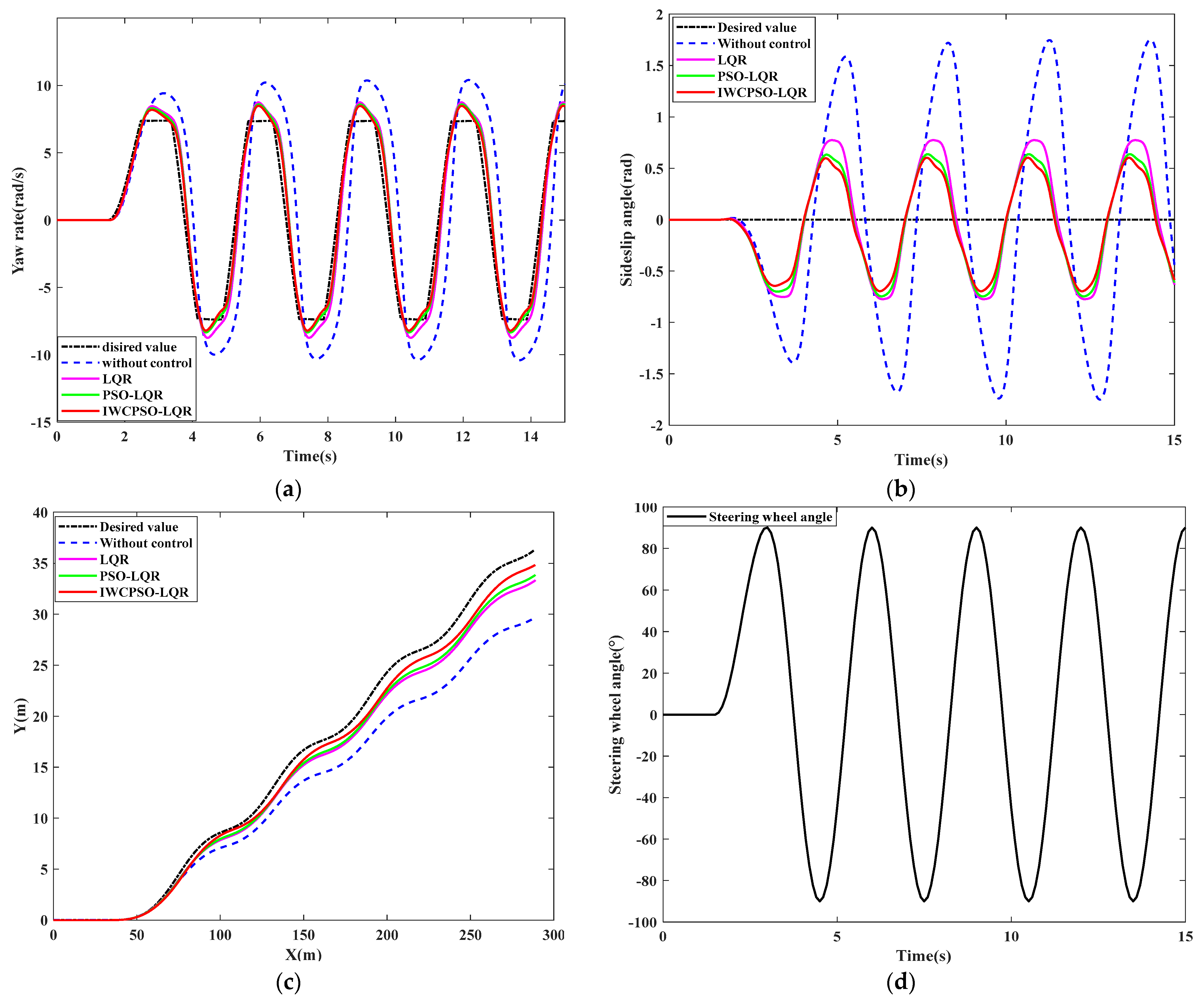
4.2.1. Sinusoidal Test on Low Adhesion Road Surfaces

The steering wheel angle input and simulation results are exhibited in Figure 7. Numerical results are summarized in

Table 2. Performance metrics data under sinusoidal conditions on low adhesion road surfaces.

Algorithm	Yaw Rate			Sideslip Angle
	S	RMSE	Peak Value	S	RMSE	Peak Value
Without control	15.52	17.77	10.36	20.01	20.85	1.73
LQR	7.04	12.34	8.74	11.36	14.36	0.79
PSO-LQR IWCPSO-LQR	6.28 5.99	11.69 10.25	8.56 8.46	10.91 10.01	12.08 11.67	0.65 0.60

.

Figure 7a illustrates the yaw rate comparison. It is obvious that the proposed IWCPSO-LQR can minimize the error between the yaw rate and the reference value with the best tracking performance. As listed in Table 2, the proposed IWCPSO-LQR performs the best with the minimum RMSE and S for the yaw rate, which outperforms the benchmark (without control) by 42.3% and 61.4%, respectively. Figure 7b gives the result of the sideslip angle. Obviously, IWCPSO-LQR exhibits the best performance among the three control methods. In addition, the RMSE and S of the sideslip angle for IWCPSO-LQR are reduced by 44% and 50% compared to the benchmark. From Figure 7a,b and Table 2, the maximum yaw rate and sideslip angle of IWCPSO-LQR are reduced by 18.3% and 65.3% in contrast to the benchmark. Figure 7c presents the control result of the trajectory tracking, indicating that the proposed IWCPSO-LQR can improve the tracking performance effectively.

For the yaw rate and sideslip angle, three performance metrics comparisons for three kinds of LQR-based control methods are demonstrated in Figure 8 and Figure 9. Figure 8 denotes that the S, RMSE and peak value of the yaw rate under the control of IWCPSO-LQR decreases by 4.62%, 12.3% and 1.17% compared with PSO-LQR, respectively. Figure 8 shows that the IWCPSO-LQR control can track the desired yaw rate well and the control effect is remarkable. As indicated in Figure 9, the S, RMSE and peak value of IWCPSO-LQR’s sideslip angle declines by 8.25%, 3.39% and 7.69% with regard to PSO-LQR, respectively. However, neither the IWCPSO-LQR nor the PSO-LQR control can make the sideslip angle always be zero without fluctuation. This is because it is difficult to achieve precise control of the lateral force. Therefore, the sideslip angle is limited in the stability zone and cannot be zero.

4.2.2. DLC Test on Low Adhesion Road Surfaces

The rapid lane change is the main application scenario of DYC; thus, the proposed control method is also evaluated in the DLC scenario. The simulation results for the DLC test on a low adhesion road are given in Figure 10. Relevant performance metrics data are listed in

Table 3. Performance metrics data under DLC on low adhesion road surfaces.

Algorithm	Yaw Rate			Sideslip Angle
	S	RMSE	Peak Value	S	RMSE	Peak Value
Without control	317.52	546.23	71.25	408.01	427.28	178.55
LQR	16.91	32.74	17.85	15.65	25.34	3.68
PSO-LQR	15.63	29.63	15.46	13.35	21.08	2.91
IWCPSO-LQR	14.96	27.99	15.14	13.08	20.74	2.64

.

From Figure 10a,b, it is obvious that, on one hand, the vehicle’s yaw rate and sideslip angle ultimately diverge completely without control, and on the other hand, the proposed IWCPSO-LQR enhances the effectiveness of the yaw rate and sideslip angle control compared with the other two strategies. As indicated in Table 3, in contrast to PSO-LQR, LQR and without control, the proposed IWCPSO-LQR optimizes 2.1%, 15.2% and 78.5% of the yaw rate’s peak value, as well as 9.3%, 28.3% and 98.5% for the sideslip angle’s peak value. Additionally, in terms of S and RMSE for the yaw rate and sideslip angle, IWCPSO-LQR also exhibits superior improvements of the vehicle stability. Excellent track performance of the vehicle is shown via DYC in Figure 10c. Among the three control methods, IWCPSO has the smallest deviation from the target trajectory.

Specifically, comparison results of performance metrics for three control methods are illustrated in Figure 11 and Figure 12. With regard to the yaw rate, the peak value, RMSE and S of IWCPSO-LQR are 2.07%, 5.53% and 4.29% lower than that of PSO-LQR. Figure 12 shows that the peak value, RMSE and S of the sideslip angle using IWCPSO-LQR is reduced by 9.28%, 1.61% and 2.0% relative to PSO-LQR. The above comparison results show that the cosine-adjustment method of inertia weight is effective to obtain global optimization results for PSO, thus having a better control effect than PSO in the upper control of DYC.

4.3. Simulation on High Adhesion Road Surfaces

To verify the adaptability of the proposed DYC method, a high adhesion coefficient road is also necessary to study.

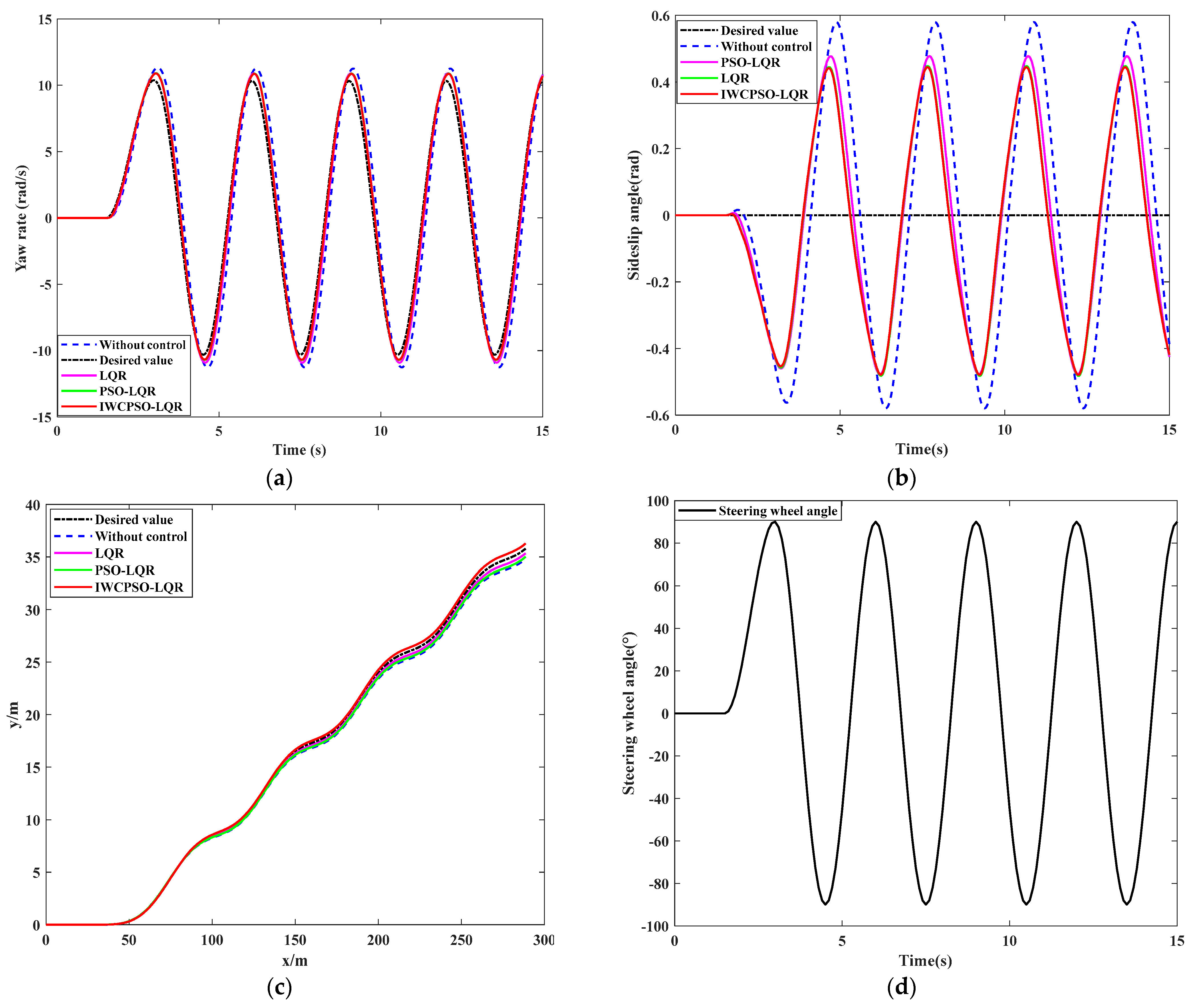
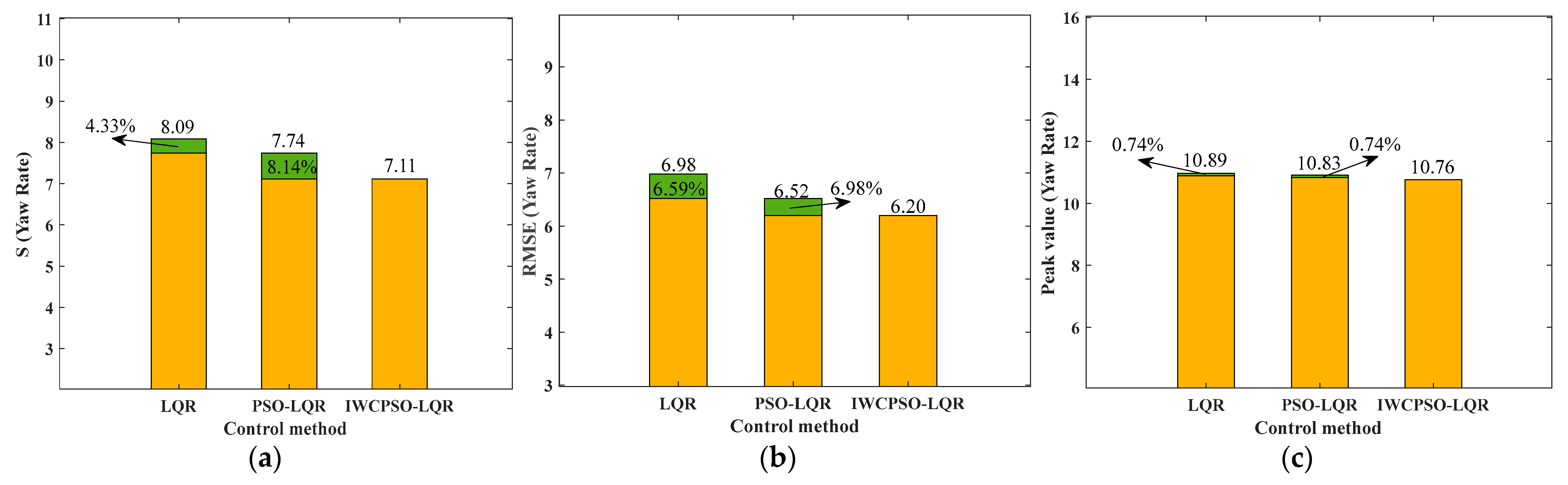
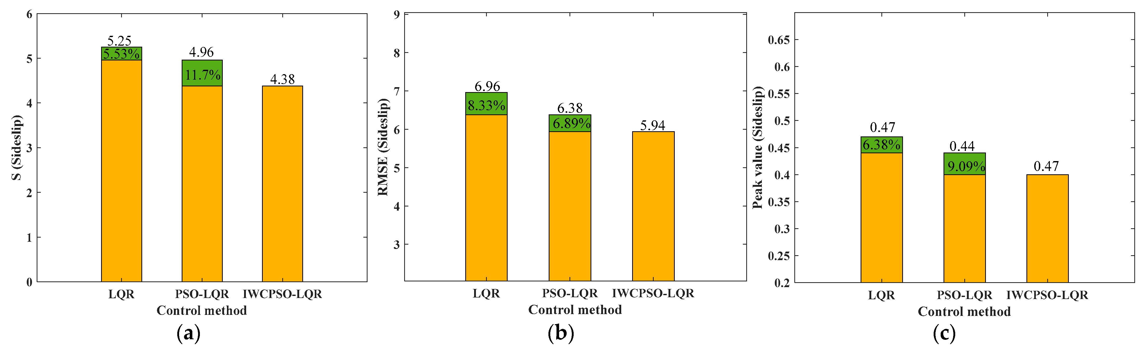
4.3.1. Sinusoidal Test on High Adhesion Road Surfaces

Figure 13a–c exhibit the response of the yaw rate, sideslip angle and trajectory under four different control methods, respectively. As shown in Figure 13a, IWCPSO-LQR has a better control effect compared with other methods in terms of the yaw rate.

Table 4. Performance metrics data under sinusoidal conditions on high adhesion road surfaces.

Algorithm	Yaw Rate			Sideslip Angle
	S	RMSE	Peak Value	S	RMSE	Peak Value
Without control	16.77	8.25	11.25	10.25	7.85	0.58
LQR	8.09	6.98	10.89	5.25	6.96	0.47
PSO-LQR	7.74	6.52	10.83	4.96	6.38	0.44
IWCPSO-LQR	7.11	6.20	10.76	4.38	5.94	0.40

demonstrates that all three performance metrics of the yaw rate for IWCPSO-LQR are the smallest, which are also the closest to the reference value. It can be noted from Figure 14 that the S, RMSE and peak value of the yaw rate under IWCPSO-LQR are reduced by 8.14%, 6.98% and 0.74% compared to PSO-LQR. The sideslip angle is illustrated in Figure 13b, indicating that the sideslip angle can be controlled within 0.48 rad under LQR-based methods compared to the without control scenario. The quantitative results of the sideslip angle’s performance metrics given in Table 4 and Figure 15 suggest that the peak value of ICWPSO-LQR has been optimized by 9.09%, 14.9% and 31% in contrast to PSO-LQR, LQR and without control. For the same comparison, the improvement is 11.7%, 16.57% and 57.27% for the S, as well as 6.89%, 14.65% and 24.33% for the RMSE. The trajectory described in Figure 13c implies that IWCPSO-LQR has a smaller deviation from the target trajectory than the LQR-based control and without control, which can enhance the tracking effects and control accuracy.

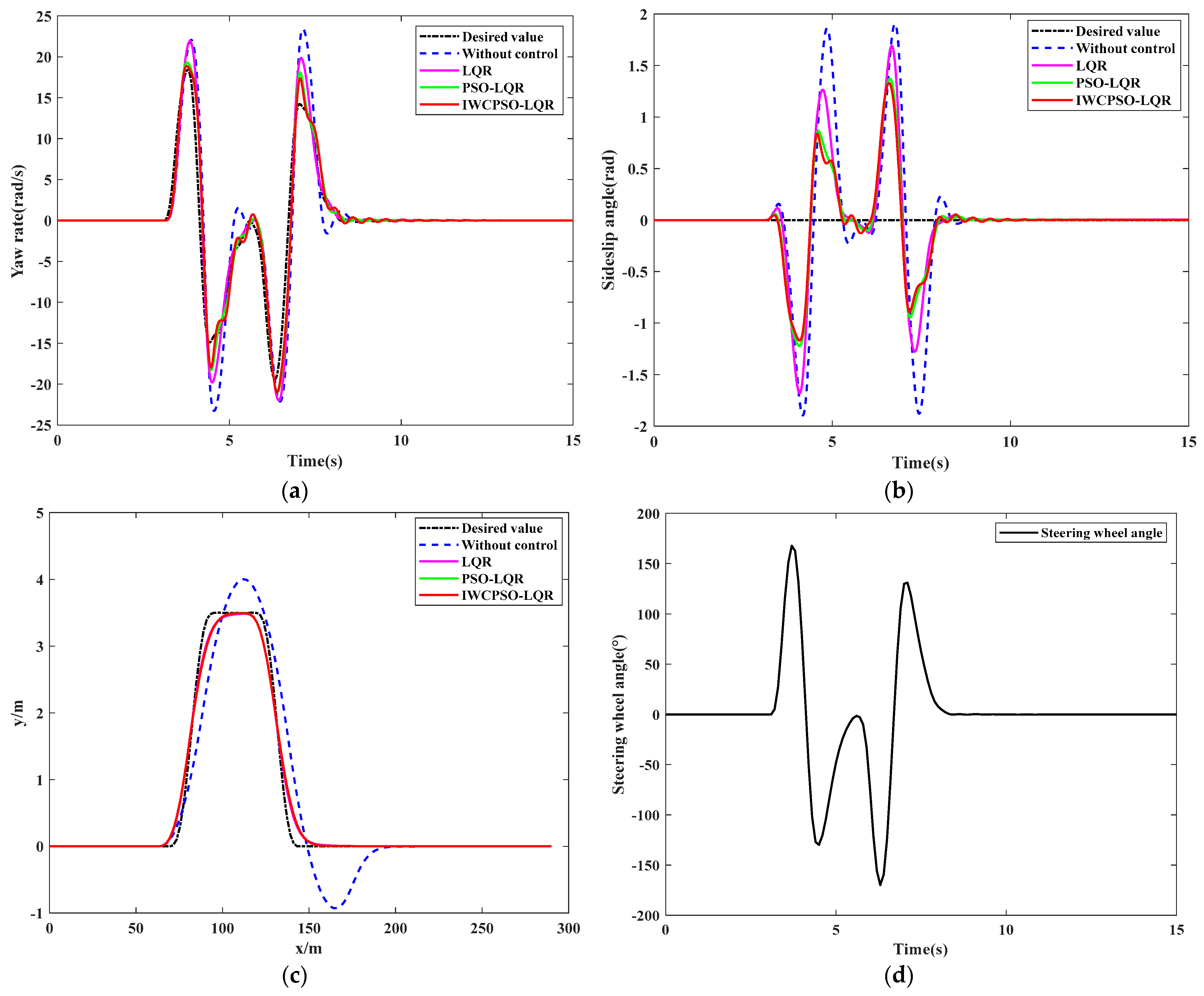
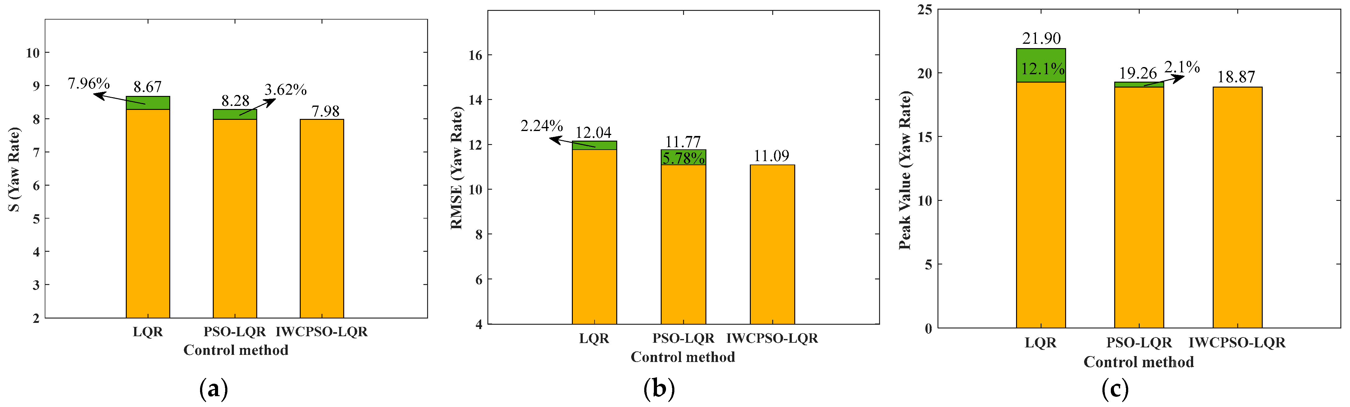
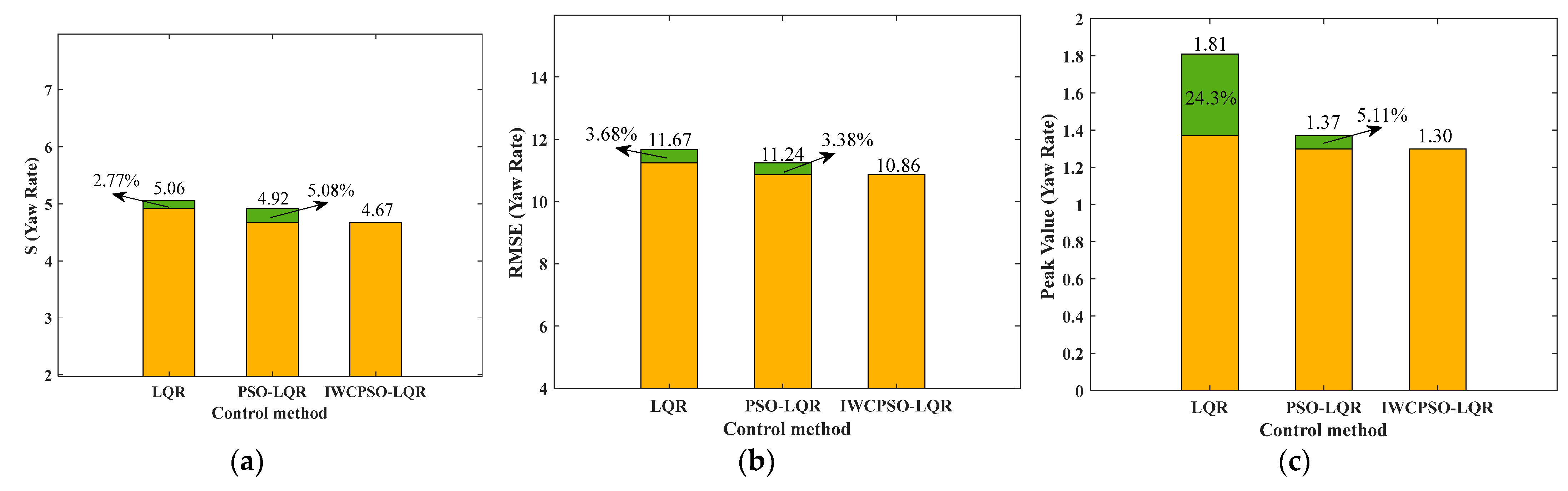
4.3.2. DLC Test on High Adhesion Road Surfaces

The response curve and specific evaluation index data are given in Figure 16, Figure 17 and Figure 18 and

Table 5. Performance metrics data under DLC on high adhesion road surfaces.

Algorithm	Yaw Rate			Sideslip Angle
	S	RMSE	Peak Value	S	RMSE	Peak Value
Without control	20.31	15.85	23.36	12.65	14.83	1.87
LQR	8.67	12.04	21.90	5.06	11.67	1.81
PSO-LQR	8.28	11.77	19.26	4.92	11.24	1.37
IWCPSO-LQR	7.98	11.09	18.87	4.67	10.86	1.30

. As analyzed in the above three test conditions, the proposed IWCPSO-LQR method still retains huge superiority under DLC on high adhesion road surfaces. Specifically, the yaw rate and sideslip angle regulated by IWCPSO-LQR sufficiently track the change of the desired value with a faster response speed during the whole test process, as depicted in Figure 16a,b. It can be viewed from Table 5 and Figure 17 that the maximum yaw rate of IWCPSO-LQR is 18.87 rad/s, which is 2.1% lower than that of PSO-LQR. For the other two performance metrics, the S and RMSE of the yaw rate under IWCPSO-LQR is 3.62% and 5.78% lower than PSO-LQR, respectively. In addition, as can be seen from Table 5 and Figure 18, the peak value of the sideslip angle for the IWCPSO-LQR method decreased more significantly, with the minimum value of 1.30 rad. Comparative analysis of LQR-based methods is concluded in Figure 18. On one hand, the S, RMSE and peak value of the sideslip angle for PSO-LQR declines by 3.62%, 5.78% and 2.10% in contrast with LQR; on the other hand, the above three indicators of the sideslip angle for IWCPSO-LQR are reduced by 2.77%, 3.68% and 24.3% compared to PSO-LQR. As shown in Figure 16c, the vehicle trajectory deviates severely from the desired trajectory in the absence of control. All three LQR-based control methods can follow the targeted trajectory well by suppressing the vehicle’s sideslip.

It can be found from DLC test on the high adhesion road that the proposed IWCPSO-LQR can make the peak value of the yaw rate and sideslip angle drop significantly. The yaw rate, sideslip angle and trajectory dominated by IWCPSO-LQR can also follow the ideal values well, which demonstrates the superiority of IWCPSO-LQR in the vehicle stability control.

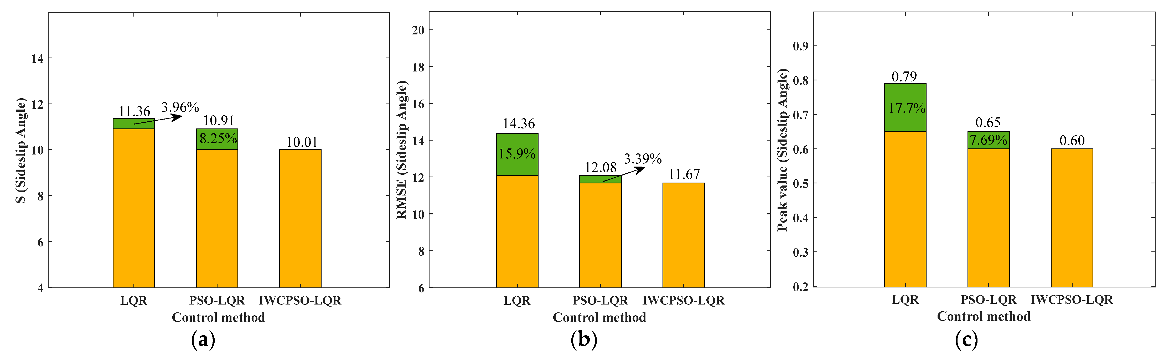
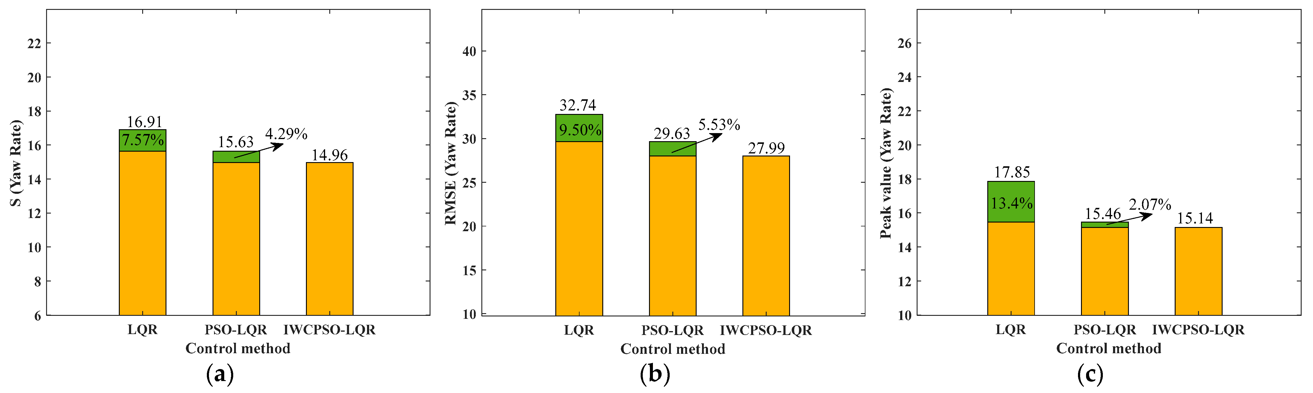
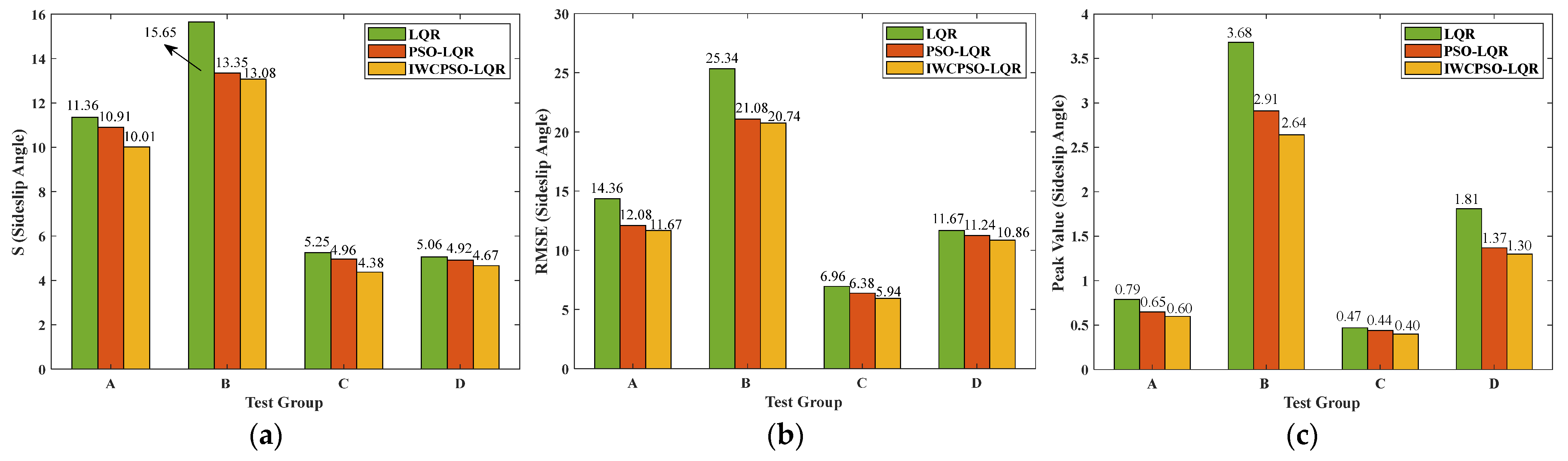
4.4. Comparison Analysis of Different Algorithms under Different Simulation Conditions

To evaluate the effectiveness of different algorithms under different simulation conditions, comparative tests of four groups were conducted, as shown in

Table 6. Four groups comparative tests.

Test Group	Test Condition	Road Adhesion Coefficient
A	Sinusoidal condition	Low (0.3)
B	Double-lane-change condition	Low (0.3)
C	Sinusoidal condition	High (0.85)
D	Double-lane-change condition	High (0.85)

. Performance metrics, including S, RMSE and the peak value of the yaw rate and sideslip angle, obtained by four test groups, composed of the sinusoidal test and DLC test under low and high adhesion road, are analyzed comparatively. The analysis results are presented in Figure 19 and Figure 20. Under four different simulation tests, three performance metrics of the yaw rate and sideslip angle controlled by the proposed IWCPSO-LQR have the smallest value among LQR, PSO-LQR and IWCPSO-LQR, which shows excellent robustness and feasibility of the proposed IWCPSO-LQR method.

5. Conclusions

A hierarchical DYC optimization control method is proposed to improve lateral stability and optimize energy consumption of 4W-DDEVs. An upper layer controller adopts IWCPSO to adjust the Q matrix parameter of LQR, while a lower layer controller employs QP to optimize the torque allocation of an individual wheel. Co-simulation analysis is performed to verify the effectiveness of the proposed hierarchical control strategy. Simulation results for two kinds of maneuvers under low and high adhesion roads show that the hierarchical control method is superior to other benchmark control methods with notable improvements on yaw rate, sideslip angle and trajectory tracking, thus improving the vehicle’s driving stability. Furthermore, the robustness and real-time of the proposed control method are also proven via simulation comparative analysis. The analysis results indicate that with IWCPSO-LQR, the S, RMSE and peak value for the yaw rate and sideslip angle outperform the benchmark by 95.2% and 96.8, 94.9% and 95.1% and 78.8% and 98.5% under DLC on the low adhesion road surface and 61.4% and 50.0%, 42.3% and 45.5% and 18.3% and 65.3% under the sinusoidal condition on the low adhesion road surface, respectively.

In future work, control algorithms with high accuracy and a fast computation speed should be incorporated into the hierarchical control framework of DYC, as well as the state observer of the sideslip angle and road adhesion coefficient, in order to further enhance the control effect. Meanwhile, both a hardware-in-loop test and road test will also be conducted to evaluate the superiority of the control algorithm.

References

1. Li, Y.; Zhang, J.; Lv, C. Coordinated control of the steering system and the distributed motors for comprehensive optimization of the dynamics performance and the energy consumption of an electric vehicle. Proc. Inst. Mech. Eng. Part D J. Automob. Eng. 2017, 231, 1605–1626. [Google Scholar] [CrossRef]
2. Deng, H.F.; Zhao, Y.Q.; Nguyen, A.T. Fault-tolerance-ant predictive control with deep-reinforcement-learning-based torque distribution for four in-wheel motor drive electric vehicle. IEEE/ASME Trans. Mechatron. 2023, 28, 668–680. [Google Scholar] [CrossRef]
3. Dang, M.; Zhang, C.W.; Yang, Z.; Chang, B.; Wang, J.L. Research on steering coordination control strategy for distributed drive electric vehicles. AIP Adv. 2023, 13, 025261. [Google Scholar] [CrossRef]
4. Ma, L.; Cheng, C.; Guo, J.F.; Shi, B.H.; Ding, S.Y.; Mei, K.Q. Direct yaw-moment control of electric vehicles based on adaptive sliding mode. Math. Biosci. Eng. 2023, 20, 13334–13335. [Google Scholar] [CrossRef]
5. Zhang, N.; Wang, J.S.; Li, Z.H.; Xu, N.; Ding, H.T.; Zhang, Z.; Guo, K.H.; Xu, H.C. Coordinated optimal control of AFS and DYC for four-wheel independent drive electric vehicles based on MAS model. Sensors 2023, 23, 3505. [Google Scholar] [CrossRef]
6. Wang, L.; Pang, H.; Wang, P.; Liu, M.H.; Hu, C. A yaw stability-guaranteed hierarchical coordination control strategy for four-wheel drive electric vehicles using an unscented Kalman filter. J. Frankl. Inst. 2023, 360, 9663–9688. [Google Scholar] [CrossRef]
7. Gao, F.; Zhao, F.K.; Zhang, Y. Research on yaw stability control strategy for distributed drive electric trucks. Sensors 2023, 23, 7222. [Google Scholar] [CrossRef]
8. Tang, H.R.; Bei, S.Y.; Li, B.; Sun, X.Q.; Huang, C.; Tian, J.; Hu, H.Z. Mechanism analysis and control of lateral instability of 4WID vehicle based on phase plane analysis considering front wheel angle. Actuators 2023, 12, 121. [Google Scholar] [CrossRef]
9. Sun, X.Q.; Wang, Y.J.; Cai, Y.F.; Wong, P.K.; Chen, L. NFTSM control of direct yaw moment for autonomous electric vehicles with consideration of tire nonlinear mechanical properties. Bull. Pol. Acad. Sci. Tech. Sci. 2021, 69, e137065. [Google Scholar] [CrossRef]
10. Viktor, S.; Paulius, K.; Eldar, Š.; Barys, S.; Valentin, I. Review of integrated chassis control techniques for automated ground vehicles. Sensors 2024, 24, 600. [Google Scholar] [CrossRef]
11. Zhang, Z.M.; Xie, L.; Lu, S.; Wu, X.L.; Su, H.Y. Vehicle yaw stability control with a two-layered learning MPC. Veh. Syst. Dyn. 2023, 61, 423–444. [Google Scholar] [CrossRef]
12. Liu, C.; Liu, H.; Han, L.J.; Wang, W.D.; Guo, C.S. Multi-level coordinated yaw stability control based on sliding mode predictive control for distributed drive electric vehicles under extreme conditions. IEEE Trans. Veh. Technol. 2023, 72, 280–296. [Google Scholar] [CrossRef]
13. Ge, P.S.; Guo, L.; Feng, J.D.; Zhou, X.Y. Adaptive stability control based on sliding model control for BEVs driven by in-wheel motors. Sustainability 2023, 15, 8660. [Google Scholar] [CrossRef]
14. Liu, W.; Zhang, Q.J.; Wan, Y.D.; Liu, P.; Yu, Y.; Guo, J. Yaw stability control of automated guided vehicle under the condition of centroid variation. J. Braz. Soc. Mech. Sci. Eng. 2022, 44, 18. [Google Scholar] [CrossRef]
15. Zhang, J.Y.; Ling, R. Hierarchical control scheme of direct yaw moment control system based on second-order sliding mode control. In Proceedings of the 2022 34th Chinese Control and Decision Conference (CCDC), Hefei, China, 21–23 May 2022. [Google Scholar]
16. Ma, L.; Mei, K.Q.; Ding, S.H. Direct yaw-moment control design for in-wheel electric vehicle with composite terminal sliding mode. Nonlinear Dyn. 2023, 111, 17141–17156. [Google Scholar] [CrossRef]
17. Cao, W.K.; Shen, X.F.; Ling, H.P. Analysis and design of direct yaw-moment control for distributed drive electric vehicles considering. In Proceedings of the 8th Asia-Pacific Conference on Intelligent Robot Systems, Xi’an, China, 7–9 July 2023. [Google Scholar]
18. Lin, J.M.; Zou, T.; Su, L.; Zhang, F.; Zhang, Y. Optimal coordinated control of active front steering and direct yaw moment for distributed drive electric bus. Machines 2023, 11, 640. [Google Scholar] [CrossRef]
19. Zhang, L.; Yu, L.Y.; Pan, N.; Liu, X.Y.; Song, J. Vehicle direct yaw moment control based on tire cornering stiffness estimation. In Proceedings of the ASME 2014 Dynamic Systems and Control Conference, San Antonio, TX, USA, 22–24 October 2014. [Google Scholar]
20. Oh, K.; Joa, E.; Lee, J.; Yun, J.; Yi, K. Yaw Stability control of 4WD vehicles based on model predictive torque vectoring with physical constraints. Int. J. Automot. Technol. 2019, 20, 923–932. [Google Scholar] [CrossRef]
21. Wu, J.Y.; Wang, Z.P.; Zhang, L. Unbiased-estimation-based and computation-efficient adaptive MPC for four-wheel-independently-actuated electric vehicles. Mech. Mach. Theory 2020, 154, 104100. [Google Scholar] [CrossRef]
22. Altork, B.; Yazici, H. Robust static output feedback H-controller design for three degree of freedom integrated bus lateral, yaw, roll dynamics model. Trans. Inst. Meas. Control 2019, 41, 4545–4568. [Google Scholar] [CrossRef]
23. Wang, R.R.; Jing, H.; Hu, C.; Yan, F.J.; Chen, N. Robust H path following control for autonomous ground vehicles with delay and data dropout. IEEE Trans. Intell. Transp. Syst. 2016, 17, 2042–2050. [Google Scholar] [CrossRef]
24. Liao, Z.L.; Cai, L.C.; Li, J.Q.; Zhang, Y.Y.; Liu, C.G. Direct yaw moment control of eight-wheeled distributed drive electric vehicles based on super-twisting sliding mode control. Front. Mech. Eng. 2023, 9, 1347852. [Google Scholar] [CrossRef]
25. Shi, K.; Yuan, X.F.; Huang, G.M.; Zhang, X.Z.; Shen, Y.P. DLMPCS-based improved yaw stability control strategy for DDEV. IET Intell. Transp. Syst. 2019, 13, 1329–1339. [Google Scholar] [CrossRef]
26. Song, Y.T.; Shu, H.Y.; Chen, X.B.; Luo, S. Direct-yaw-moment control of four-wheel-drive electrical vehicle based on lateral tire-road forces and sideslip angle observer. IET Intell. Transp. Syst. 2019, 13, 303–312. [Google Scholar] [CrossRef]
27. Hang, P.; Chen, X.B. Integrated chassis control algorithm design for path tracking based on four-wheel steering and direct yaw-moment control. Proc. Inst. Mech. Eng. 2019, 233, 625–641. [Google Scholar] [CrossRef]
28. Guo, N.Y.; Lenzo, B.; Zhang, X.D.; Zou, Y.; Zhai, R.Q.; Zhang, T. A real-time nonlinear model predictive controller for yaw motion optimization of distributed drive electric vehicles. IEEE Trans. Veh. Technol. 2020, 69, 4935–4946. [Google Scholar] [CrossRef]
29. Liang, J.H.; Feng, J.W.; Lu, Y.B.; Yin, G.D.; Zhuang, W.C.; Mao, X. A direct yaw moment control framework through robust T-S fuzzy approach considering vehicle stability margin. IEEE-ASME Trans. Mechatron. 2024, 29, 166–178. [Google Scholar] [CrossRef]
30. Wu, X.J.; Zhou, B.; Wu, T.Y.; Pan, Q.X. Research on intervention criterion and stability coordinated control of AFS and DYC. Int. J. Veh. Des. 2022, 90, 116–141. [Google Scholar] [CrossRef]
31. Lu, C.Y.; Shih, M.C. Application of the Pacejka magic formula tyre model on a study of a hydraulic anti-lock braking system for a light motorcycle. Veh. Syst. Dyn. 2004, 41, 431–448. [Google Scholar] [CrossRef]
32. Khasawneh, L.; Das, M. A robust electric power-steering-angle controller for autonomous vehicles with disturbance rejection. Electronics 2022, 11, 1337. [Google Scholar] [CrossRef]
33. Song, J. Integrated control of brake pressure and rear-wheel steering to improve lateral stability with fuzzy logic. Int. J. Automot. Technol. 2012, 13, 563–570. [Google Scholar] [CrossRef]
34. Clerc, M.; Kennedy, J. The particle swarm—Explosion, stability, and convergence in a multidimensional complex space. IEEE Trans. Evol. Comput. 2002, 6, 58–73. [Google Scholar] [CrossRef]
35. Wang, D.S.; Tan, D.P.; Liu, L. Particle swarm optimization algorithm: An overview. Soft Comput. 2018, 22, 387–408. [Google Scholar] [CrossRef]
36. Lin, A.P.; Liu, D.; Li, Z.Q.; Hasanien, H.M.; Shi, Y.T. Heterogeneous differential evolution particle swarm optimization with local search. Complex Intell. Syst. 2023, 9, 6905–6925. [Google Scholar] [CrossRef]
37. Chen, S.H.; Zhang, C.Q.; Yi, J.P. Time-optimal trajectory planning for woodworking manipulators using an improved PSO algorithm. Appl. Sci. 2023, 13, 10482. [Google Scholar] [CrossRef]
38. ISO3888-2:2018; Passenger Cars–Test Track for A Severe Lane–Change Manoeuvre–Part 1: Double Lane–Change. International Organization for Standardization (ISO): Geneva, Switzerland, 2018.
39. ISO15037-1:2019; Road Vehicles–Vehicle Dynamics Test Methods–Part 1: General Conditions for Passenger Cars. International Organization for Standardization (ISO): Geneva, Switzerland, 2019.
Figure 1. 2-DOF reference model.
Mathematics 12 01715 g001
Figure 2. 7-DOF vehicle model.
Mathematics 12 01715 g002
Figure 3. Hierarchical control framework of direct-yaw-moment control system.
Mathematics 12 01715 g003
Figure 4. Change process of inertia factor.
Mathematics 12 01715 g004
Figure 5. Optimization flow of IWCPSO algorithm.
Mathematics 12 01715 g005
Figure 6. Block diagram of simulation test flow.
Mathematics 12 01715 g006
Figure 7. Performance comparison of different upper controllers under sinusoidal conditions on low adhesion road surfaces. (a) Yaw rate; (b) sideslip angle; (c) trajectory; (d) steering wheel angle.
Mathematics 12 01715 g007
Figure 8. Objective performance metrics of sinusoidal test on low adhesion road surfaces for yaw rate. (a) S; (b) RMSE; (c) peak value.
Mathematics 12 01715 g008
Figure 9. Objective performance metrics of sinusoidal test on low adhesion road surfaces for sideslip angle. (a) S; (b) RMSE; (c) peak value.
Mathematics 12 01715 g009
Figure 10. Performance comparison of different upper controllers under DLC on low adhesion road surfaces. (a) Yaw rate; (b) sideslip angle; (c)trajectory; (d) steering wheel angle.
Mathematics 12 01715 g010
Figure 11. Objective performance metrics of DLC test on low adhesion road surfaces for yaw rate. (a) S; (b) RMSE; (c) peak value.
Mathematics 12 01715 g011
Figure 12. Objective performance metrics of DLC test on low adhesion road surfaces for sideslip angle. (a) S; (b) RMSE; (c) peak value.
Mathematics 12 01715 g012
Figure 13. Performance comparison of different upper controllers under sinusoidal conditions on high adhesion road surfaces. (a) Yaw rate; (b) sideslip angle; (c) trajectory; (d) steering wheel angle.
Mathematics 12 01715 g013
Figure 14. Objective performance metrics of sinusoidal test on high adhesion road surfaces for yaw rate. (a) S; (b) RMSE; (c) peak value.
Mathematics 12 01715 g014
Figure 15. Objective performance metrics of sinusoidal test on high adhesion road surfaces for sideslip angle. (a) S; (b) RMSE; (c) peak value.
Mathematics 12 01715 g015
Figure 16. Performance comparison of different upper controllers under DLC on high adhesion road surfaces. (a) Yaw rate; (b) sideslip angle; (c)trajectory; (d) steering wheel angle.
Mathematics 12 01715 g016
Figure 17. Objective performance metrics of DLC test on high adhesion road surfaces for yaw rate. (a) S; (b) RMSE; (c) peak value.
Mathematics 12 01715 g017
Figure 18. Objective performance metrics of DLC test on high adhesion road surfaces for sideslip angle. (a) S; (b) RMSE; (c) peak value.
Mathematics 12 01715 g018
Figure 19. Objective performance metrics of yaw rate under different test groups. (a) S; (b) RMSE; (c) peak value.
Mathematics 12 01715 g019
Figure 20. Objective performance metrics of sideslip angle under different test groups. (a) S; (b) RMSE; (c) peak value.
Mathematics 12 01715 g020