Abstract
This paper investigates the bumpless transfer control of linear switched positive systems based on state and disturbance observers. First, state and disturbance observers are designed for linear switched positive systems to estimate the state and the disturbance. By combining the designed state observer, the disturbance observer, and the output, a new controller is constructed for the systems. All gain matrices are described in the form of linear programming. By using co-positive Lyapunov functions, the positivity and stability of the closed-loop system can be ensured. In order to achieve the bumpless transfer property, some additional sufficient conditions are imposed on the control conditions. The novelties of this paper lie in that (i) a novel framework is presented for positive disturbance observer, (ii) double observers are constructed for linear switched positive systems, and (iii) a bumpless transfer controller is proposed in terms of linear programming. Finally, two examples are given to illustrate the effectiveness of the proposed results.
Keywords:
linear switched positive systems; disturbance observe; bumpless transfer control; linear programming MSC:
93C28
1. Introduction
Positive systems are an important class of systems whose states and outputs are always non-negative for any non-negative initial states and inputs. They have been covered in [1,2,3] and are widely used in applications such as water systems [4], ecology [5], industrial engineering [6], and so on. Linear switched positive systems (SPSs) are a class of hybrid systems consisting of a finite number of positive subsystems and a switching rule. The stability and stabilization of SPSs have attracted great attention [7,8,9,10]. For general (nonpositive) switched systems, quadratic Lyapunov functions are commonly used [11,12,13,14]. Owing to the positivity requirement, quadratic Lyapunov functions are not the best choice for SPSs. It has also been verified that the co-positive Lyapunov function (CLF) is more suitable for SPSs [7,8,9,10]. In [9], a common CLF was constructed for the exponential stability of SPSs. For discrete-time SPSs, Liu constructed a switched CLF to reduce the conservativeness of common CLF [15]. In [16], multiple CLFs and average dwell time (ADT) switching were first introduced for SPSs. The work in [17] discusses the stability in terms of CLF and further designs a state-feedback controller. Existing results verify that CLF is powerful for handling the issues of SPSs.
The observer technique is widely used in switched systems [18], multiagent systems [19], nonlinear systems [20], etc. For positive systems, there are a number of features that are different from general systems. Thus, the utilization of a state observer in positive systems is also different from general systems. In [21], a Luenberger-type observer was designed for positive systems using linear programming. In [22], a novel design approach to the observer and a static state-feedback controller were presented for positive systems characterized by interval uncertainties and time delay. It should be noted that the observer of positive systems must also exhibit positivity. This point arises from the fact that a negative attribute within the output of observer is inadequate for accurately estimating the non-negative state. Different from positive systems, the observer of SPSs has to consider not only the positivity but also the effects of the switching signal on the observer. In [23], two types of interval switched positive observers were introduced for discrete-time SPSs. In [24], asynchronous observers were presented for SPSs. In the above literature, disturbance factor was assumed to be unmeasurable and set as a disturbance signal. For example, the work in [24] discussed the performance of the systems with regard to the disturbance. The disturbance attenuation performance can achieve some prescribed attenuation effects for the disturbance. However, it cannot accurately estimate the disturbance. The lack of disturbance information may deteriorate the system performance. The estimation of disturbance was one of effective strategies to acquire disturbance information in [25]. In [26], the problem of disturbance attenuation in stochastic systems was solved by introducing a disturbance observer. In positive systems, the work in [27] provides descriptions of the utilization of disturbance observers in positive disturbances. For positive Markovian jump systems, a linear-programming-based disturbance observer was designed in [28]. The work in [29] proposed an event-triggered disturbance-observer-based controller to ensure the positivity and stability of SPSs. A situation where both states and disturbances are unmeasurable is not considered in the aforementioned literature. Therefore, it needs to design both state and disturbance observers simultaneously. Some issues arise, such as (i) how to jointly design the state and disturbance observers, (ii) how to construct a double-observer-based controller, and (iii) how to describe the corresponding conditions in a tractable form.
For switched systems, there exist transient bumps when the switching occurs. The signal bump is a specific behavior of switched systems. With increasing demands on the accuracy of switched systems, the effects caused by transient bumps need to be eliminated. As a result, bumpless transfer control was proposed to ensure the smooth switching of the systems by adopting appropriate control strategies [30,31,32]. This can avoid negative effects caused by the signal bump, such as system performance damage, equipment failure, etc. For switched linear parameter-varying systems, an bumpless transfer control method was presented in [33,34]. The work in [35] proposed a control strategy based on mode-dependent ADT and bumpless transfer to achieve stability in switched positive delayed nonlinear systems. By virtue of event-triggered strategies, the work in [36] introduced an event-triggered bumpless transfer controller. The work in [37] applied the bumpless transfer control of switched systems for aerospace engines. In [38], a bumpless transfer feedback controller was proposed for SPSs, which can ensure a lower control signal bump caused by the switching and guarantee the -gain performance of the systems. Note that few results exist on state and disturbance observer-based bumpless transfer control of SPSs. How to design a double-observer-based bumpless transfer controller of SPSs motivates us to carry out this work.
This paper aims to deal with the problem of the bumpless transfer control of SPSs by building a state observer and a disturbance observer. First, a state observer and a disturbance observer are established based on the matrix decomposition technique, respectively. Then, a controller is designed by means of the estimated states and disturbances. Meanwhile, the bumpless transfer property of the controller is considered by imposing some conditions on the controller. The rest of this paper is presented as follows. Section 2 gives some preliminaries. In Section 3, the main results are presented. Section 4 provides two examples to verify the effectiveness of the presented results. Section 5 concludes this paper.
2. Preliminaries
Consider the following linear switched system:
where and represent the system state, the system input, the disturbance, and the output, respectively, is the switching law and takes values from a finite set , and it is continuous from the right everywhere for a switching sequence . In this paper, it is assumed that control signals and disturbances in SPSs are continuous and the disturbance in the system (1) is non-negative. Assume that is a Metzler matrix and , , , .
Some definitions and lemmas are introduced for the facilitation of later developments.
Definition 1
([1]). A system is said to be positive if all its states and outputs are non-negative for any nonnegative initial conditions.
Lemma 1
([1,2]). A matrix A is a Metzler matrix if and only if there exists a scalar δ such that .
Lemma 2
([1,3]). The system is positive if and only if is a Metzler matrix, and , , , .
Lemma 3
([1,3]). For a positive system , the following statements are equivalent:
- (i)
- The matrix A is a Hurwitz matrix;
- (ii)
- There exists a vector such that ;
- (iii)
- The system is stable.
Definition 2
([1]). For a switching signal and , denote the switching number of by . If
holds for and , then is an ADT of the switching signal and is the chatter bound.
Definition 3
([30]). Given a reference controller: , the system (1) is said to have bumpless transfer performance if the condition:
holds, where and are the state and disturbance observer states to be designed later, , , and are given scalars called the bumpless transfer performance level, , , and are given matrices with compatible dimension, and and are the jth element of and .
Notation 1.
, and represent the sets of n-dimensional vectors, non-negative vectors, and real matrices, respectively. ℵ and represent the sets of non-negative and positive integers, respectively. A matrix symbolizes the n-dimensions identity matrix. The symbols ≻ and ⪰ hold for components. Define and . p stands for the switching signal . Symbols p and q denote different subsystems.
Remark 1.
The term represents an objective control law and it is dependent on a given gain matrix . One can choose the gain matrix based on additional factors, such as practical desire, limitation of element, etc. The main objectives of the introduction of are to satisfy practical requirements and reduce the fluctuations of the designed controller.
3. Main Results
State and disturbance observers of SPSs are first designed in this section. Then, the bumpless transfer is achieved in the second subsection.
3.1. State and Disturbance Observers
The disturbance is generated by the exogenous system:
where is the state of the exogenous system, , , and is a Metzler matrix.
The disturbance observer is constructed as
where is the state of the disturbance observer and , , and are the observer gains to be designed. By Lemma 2, the exogenous system is positive. The disturbance estimation will be obtained by estimating the state .
The state observer of system (1) is designed as
where is the observer state, is the estimate of disturbance, and , , and are the observer gains to be designed.
Define the errors: and . Then, the error system can be described as
Theorem 1.
If there exist constants , , , , , , vectors , , , , , , and vectors , , , , , such that
hold , , then the observers (2) and (3) with gain matrices:
are positive, and the error system (4) is positive and asymptotically stable under the ADT switching satisfying
Proof.
First, the positivity of the observers (2) and (3) is addressed. From (5a,b) and (6), we have , , , and . Then, the system (4) can be transformed into
From (5d,e), it follows that
Together with (6) gives and . By Lemma 1, and are Metzler matrices. By (5c), we have . By , , and (5b), it is easy to be obtained that . By Lemma 2, the error system (4) is positive. Since and , then and . Thus, the observers (2) and (3) are positive.
Choose a multiple CLF: , where and . Give a switching sequence , where and . By (8), it yields that
Using (5i,j) and (6) gives
Together with (5f,g) and (11), it deduces that
Then,
Using (5i,j) and (6) gives
By (5h), (6) and (13), the following inequality holds:
Then,
By (10), (12) and (14), we have
Taking integration both sides of (15) yields that
for . Combining (5k) and gives
that is,
Repeating (15)–(18), the following relation holds:
Noting Definition 2 and , the inequality can be transformed into
where and . By (7), . Then, the error system (4) is asymptotically stable. □
Remark 2.
Noting the condition (5b) in Theorem 1, it can be derived that . If the term is removed, the condition (5b) becomes the equation . The equation is rigorous, and thus the validity of other conditions in (5) may not be guaranteed.
Remark 3.
In [21,22,23,24], the works focused on state observer of positive systems. The disturbance observer issue of SPSs is open, and few results are devoted to this issue. The obstacles to deal with this issue contain three aspects. First, a framework on double observers needs to be constructed. How to integrate the positivity restriction into the double observers is one of the difficult points. Moreover, the state observer and the disturbance observer interact with each other. Therefore, a Luenberger-type observer may not be directly applied for the double observers. Second, the question of how to design the observer gain matrices arises. For positive systems, it is interesting to present some alternative design approaches to the gain design. Under the double observers framework, the corresponding gain design refers to the state and disturbance observer gains. They are more complex than the single-state observer design. Finally, how to design the double-observer-based controller is another difficult point. Up to now, there have been no referable approaches to design a double-observer-based controller of SPSs. The key point of the design is to transform all conditions into tractable ones. Thus, some reliable computation methods can be employed to solve these conditions. Therefore, it is not easy to solve the problem of double observers design.
Remark 4.
In (2) and (3), the disturbance and state observers are constructed, respectively. It can be found that the two observers are correlated. Such observer forms have differences from the Luenberger-type observer. In (6), all gain matrices are described in the form of vector variables. Thus, the conditions in (5) can be easily formulated in the form of linear programming. Finally, the CLF is chosen to analyze the stability of the error dynamic systems. Theorem 1 develops the CLF integrated with linear programming approach to the double observers design of SPSs. It further verifies that the effectiveness of the linear approach in handling the issues of positive systems.
3.2. Bumpless Transfer Control
In this subsection, a double-observer-based bumpless transfer control design is proposed. For the state-observer-based control of SPSs, it is easy to utilize the traditional control form [23]. However, it fails to develop for the double-observer-based control of SPSs when the disturbance observer is introduced. Therefore, a novel controller form is given as
where is the estimation of , is the estimation of , and , and and are controller gain matrices to be determined later. In general, it is unnecessary to add the output term in the controller (19). Under the double observers framework, the control design will fail without the output term. Therefore, the output is added in (19).
With the controller (19) and the error system (4), the closed-loop system can be described as
Theorem 2.
If there exist constants , , , , , , , vectors , , vectors , , , , , , , , , , and vectors , , , , , , , such that the conditions (5a–e,i,j), and
and
hold for and , , with p and q denoting the different subsystems in the SPS (1), then the observers (2) and (3) with the gain matrices (6) are positive and the system (1) is positive, asymptotically stable, and reaches the bumpless transfer performance under the controller (19) with the gain matrices:
and the ADT switching satisfying (7).
Proof.
From (21a), it can be obtained that . Then, the system (20) can be transformed into
where . From (21b), it follows that Together with (23), it gives that , which implies that is Metzler matrix by Lemma 1. From and , it is easy to know that . By (21c), , and , it can be obtained that . By Theorem 1, it is clear that and are Metzler matrices and . Therefore, the error system (20) is positive by Lemma 2.
Choose a multiple CLF , where and . Give a switching sequence , where and . Then,
Using (21h) gives Together with (21d), it yields that
Then, Together with (11) and (21e,f), it gives
Then, . By (21g), we can obtain that
Then, Then, . Taking integration from both sides yields that for . The rest of the proof for the stability can be obtained by using a similar method to Theorem 1 and is omitted.
Finally, consider the bumpless transfer performance. By Definition 3, it is derived that
where stands for the jth row element of K and is the jth row element of . By , , (22a), and (22b), we have and . By , , (22c), and (22d), it is not hard to know that and . Based on and , it can be obtained that . By (22e) and (22f), we obtain that and Then, we have Thus, the considered system (1) has the bumpless transfer performance by Definition 3. □
Remark 5.
Bumpless control has been applied for switched systems [30]. In [38], the asynchronous bumpless control was explored for SPSs in terms of linear matrix inequalities. Theorem 2 further utilizes the CLF and linear programming to investigate the bumpless control of SPSs. Different from the gain performance presented in [39], Theorem 2 introduces the state and disturbance observers. Under the disturbance observer framework, the asymptotic stability and bumpless transfer control are simultaneously reached.
Remark 6.
This paper designs a double observer and double-observer-based bumpless transfer controller. There are three main difficulties to handle the considered issues. First, how to construct a novel framework on double observers and the corresponding controller of SPSs? Second, how to design the gain matrices of observer and controller? Third, how to guarantee the positivity and stability of observers and the closed-loop systems? In the existing literature [10,13,14], quadratic the Lyapunov function and linear matrix inequalities are usually used. For positive systems, some novel approaches need to be introduced owing to the positivity requirement. Therefore, it is not easy to solve the considered problems. Moreover, it is also clear that the gain design approach in (6) and the corresponding conditions in (5) are different from those in [26,31,32].
In Theorem 2, the parameters , and are required to be known. How to choose the parameters is important to Theorem 2. To provide a feasible algorithm for choosing parameters and computing the conditions in Theorem 2, Algorithm 1 is presented. Algorithm 1 aims to search parameters satisfying the conditions (21a–i) in Theorem 2. First, an empty set is defined to store the parameters that satisfy the corresponding conditions and and are initialized to their lower bounds. Then, Algorithm 1 utilizes loops to iterate through all possible values of and . Finally, these parameters will be released when the parameters satisfy conditions in (21).
| Algorithm 1 Searching parameters of Theorem 2 |
| Input: ; ; , , , , , , , ; |
| Output: ; |
| 1: Define a set ; Initialize parameters , , , and ; |
| 2: while do |
| 3: repeat |
| 4: repeat |
| 5: repeat |
| 6: if (21a)-(21i) are feasible, |
| 7: then save , and to |
| 8: end |
| 9: ; |
| 10: until ; ; |
| 11: until ; ; |
| 12: until ; ; |
| 13:end |
4. Illustrative Examples
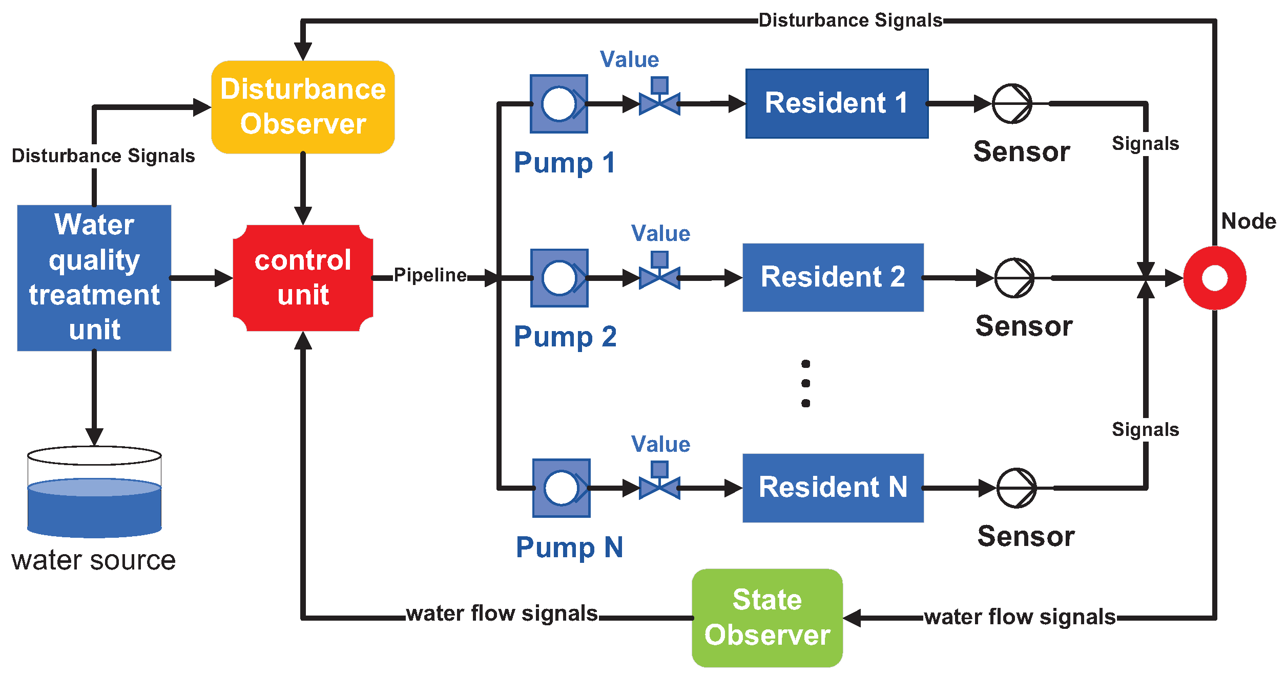
With the increase in urbanization levels, urban populations have been steadily saturating. This leads to a growing demand for water. As a result, urban water supply systems (UWSSs) face significant pressure. In [39], some findings on UWSSs were summarized. Improving the supply ability of UWSSs can reduce resource waste and energy consumption and ensure the stability of water supply pressure [40,41,42]. Figure 1 shows the relationship between observers, water flow, and residents in a UWSS. Considering the non-negativity of water flow and the switching characteristics exhibited by the changing resident water data, the UWSSs can be abstracted into SPSs. In practice, it is not easy to measure the water consumption of residents. Meanwhile, water supply systems are inevitably affected by disturbances such as damaged pipelines, weather, and so on. Therefore, it is necessary to establish both state and disturbance observers for UWSSs. Finally, it is reasonable to employ a bumpless controller to minimize the effects of water flow bump during controller switching. Considering the points mentioned above, a UWSS model is described as follows:
where denotes water consumption data of users, denotes the double-observer-based bumpless controller, is the external disturbance in UWSS, such as water flow instability caused by insufficient water pressure, and represents the th subsystem. A state observer and a disturbance observer are designed in (2) and (3). For the th subsystem of the UWSS, the control law is designed as
where denotes the estimate of user data and denotes the estimate of disturbance.
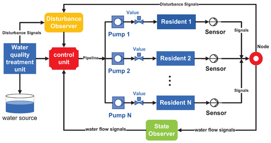
Figure 1.
The structure chart of urban water supply systems.
Example 1.
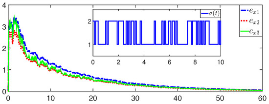
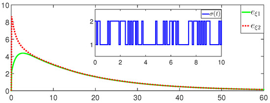
The system matrices in system (26) are
and
Choose , and . By Theorem 1, we have , and the observer gain matrices in
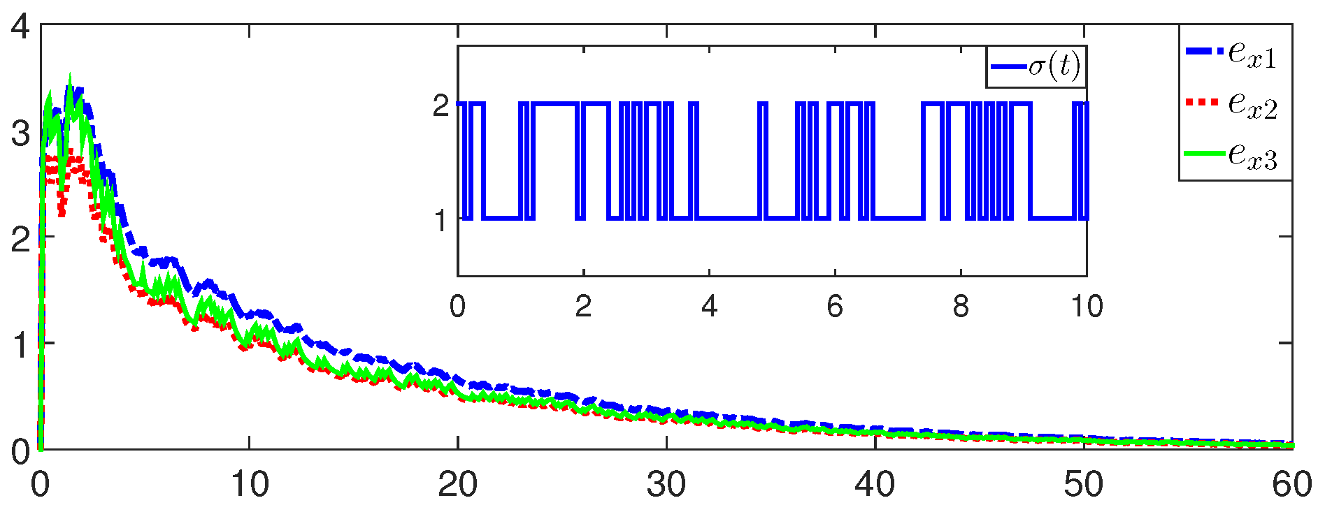
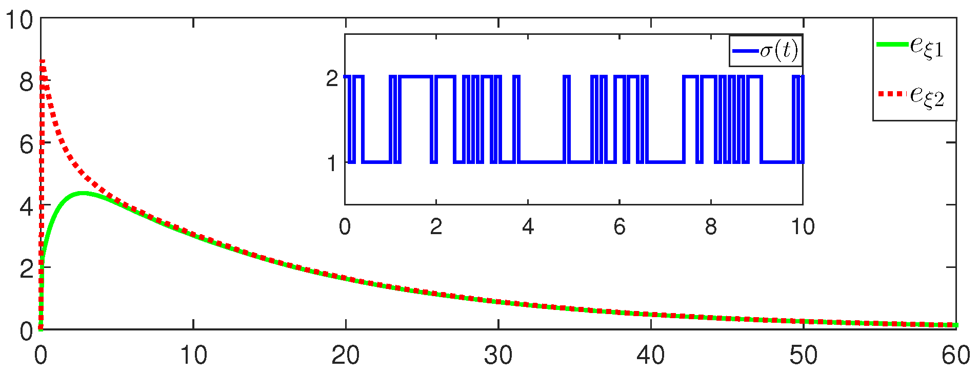
The example provides an SPS with two subsystems. In the figures, a switching signal value of 1 indicates that the first subsystem is working, while a switching signal value of 2 means that the second subsystem is working. Figure 2 shows the simulations of the errors under ADT switching. Figure 3 presents the errors under ADT switching. Figure 2 and Figure 3 show that the established state observer and disturbance observer can work. Therefore, it can be concluded that the dual observer framework based on states and disturbance is feasible in SPSs.
Figure 2.
The errors under ADT switching.
Figure 3.
The errors under ADT switching.
Example 2.
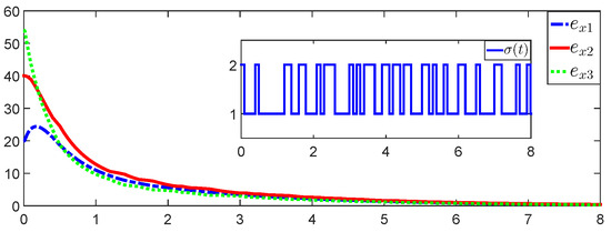

Consider the system (26) with two subsystems:
and
Choose , and . Moreover, the reference value for the controller gain matrices , , and are given as
and
By Theorem 2, we have , and the observer gain matrices in
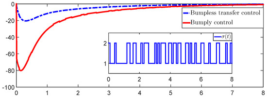
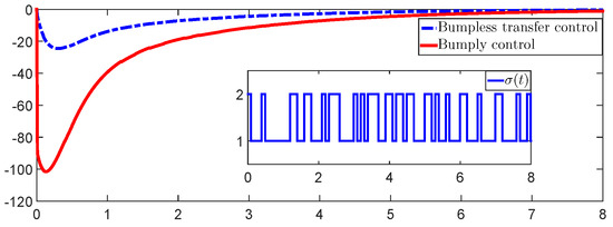
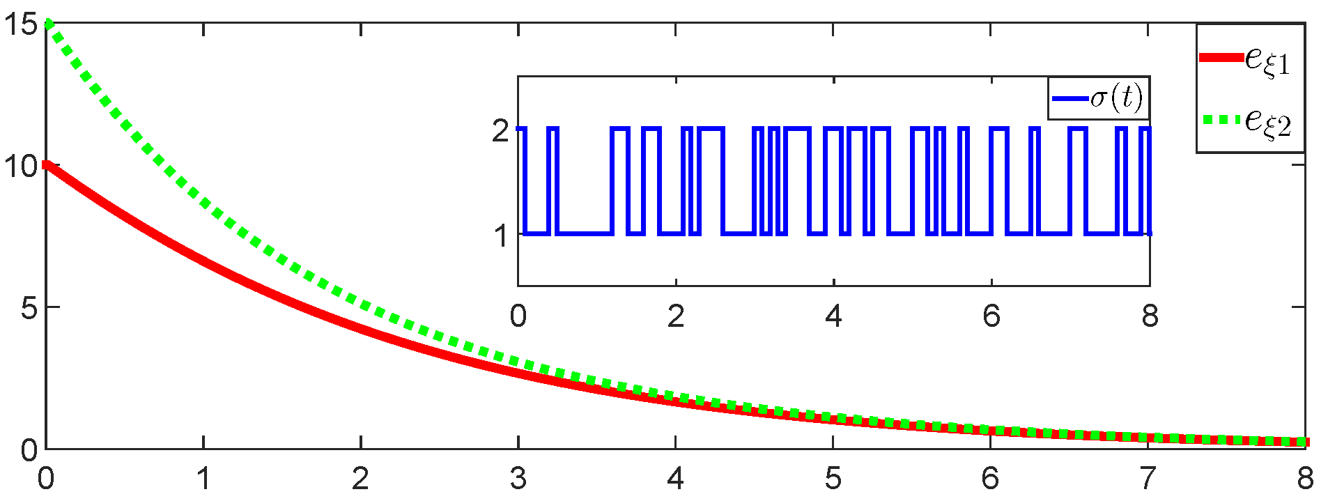
Figure 4 and Figure 5 show the simulations of the errors and under ADT switching, respectively. Figure 6 and Figure 7 present the simulations of the control signals under the bumpless transfer control and bumpy transfer control. It can be found from Figure 6 and Figure 7 that the bumpless transfer controllers have smaller fluctuations than the bumpy transfer controllers. Additionally, a comparison between Examples 1 and 2 shows that without the bumpless transfer controller, the error system has more bumps when the system is switching.
Figure 4.
The error under ADT switching.
Figure 5.
The error under ADT switching.
Figure 6.
Bumplessand bumpy transfer controllers of the first subsystem.
Figure 7.
Bumpless and bumpy transfer controllers of the second subsystem.
5. Conclusions
This paper investigates the bumpless transfer control of SPSs by virtue of state and disturbance observers. A novel framework of positive double observers is developed for SPSs. A bumpless transfer controller is proposed based on the double observers. Linear-programming-based conditions are presented, and CLF is used for the stability analysis. In the future, it will be interesting to develop more accurate bumpless transfer conditions to limit bumps in switching systems. Moreover, it is also important to discuss applications of dual observers in different switching forms.
Author Contributions
Conceptualization, Z.H. and P.Z.; methodology, Y.Y.; software, Y.Y.; validation, Y.Y. and P.Z.; formal analysis, Z.H.; investigation, Y.Y., P.Z. and Z.H.; resources, Y.Y. and Z.H.; data curation, Z.H.; writing—original draft preparation, Y.Y. and P.Z.; writing—review and editing, Z.H.; visualization, Y.Y. and P.Z.; supervision, Z.H.; project administration, P.Z. and Z.H. All authors have read and agreed to the published version of the manuscript.
Funding
This work was supported by Joint Fund of Ministry of Education for Equipment Pre-Research (8091B032253), Academician Innovation Platform Special Research Project of Hainan Province (YSPTZX202209), Key research and development project of Hainan province (ZDYF2024GXJS025), Independent Innovation Fund of Tianjin University-Hainan University (XJ2300003470), and Research Startup Fund of Hainan University (RZ2300002747).
Institutional Review Board Statement
Not applicable.
Informed Consent Statement
Not applicable.
Data Availability Statement
Data are contained within the article.
Conflicts of Interest
The authors declare no conflicts of interest. The funders had no role in the design of the study; in the collection, analyses, or interpretation of data; in the writing of the manuscript; or in the decision to publish the results.
References
- Farinan, L.; Rinaldi, S. Positive Linear Systems: Theory and Applications; Wiley: New York, NY, USA, 2000. [Google Scholar]
- Kaczorek, T. Positive 1D and 2D Systems; Springer: London, UK, 2002. [Google Scholar]
- Luenberger, D.G. Introduction to Dynamic Systems; Wiley: New York, NY, USA, 1979. [Google Scholar]
- Zhang, J.; Jia, X.; Zhang, R. Parameter-dependent Lyapunov function based model predictive control for positive systems and its application in urban water management. In Proceedings of the IEEE 2017 36th Chinese Control Conference, Dalian, China, 26–28 July 2017; pp. 4573–4578. [Google Scholar]
- Caswell, H. Matrix Population Models: Construction, Analysis, and Interpretation; Sinauer Associates: Sunderland, MA, USA, 2001. [Google Scholar]
- Caccetta, L.; Foulds, L.; Rumchev, V. A positive linear discrete-time model of capacity planning and its controllability properties. Math. Comput. Model. 2004, 40, 217–226. [Google Scholar] [CrossRef]
- Chen, G.; Yang, Y. Finite-time stability of switched positive linear systems. Int. J. Robust Nonlinear Control 2014, 24, 179–190. [Google Scholar] [CrossRef]
- Blanchini, F.; Colaneri, P.; Valcher, M. Co-positive Lyapunov functions for the stabilization of positive switched systems. IEEE Trans. Autom. Control 2012, 57, 3038–3050. [Google Scholar] [CrossRef]
- Mason, O.; Shorten, R. On linear co-positive Lyapunov functions and the stability of switched positive linear systems. IEEE Trans. Autom. Control 2007, 52, 1346–1349. [Google Scholar] [CrossRef]
- Xu, Y.; Dong, J.; Lu, R. Stability of continuous-time positive switched linear systems: A weak common copositive Lyapunov functions approach. Automatica 2018, 97, 278–285. [Google Scholar] [CrossRef]
- Huang, C.; Long, L. Safety-critical model reference adaptive control of switched nonlinear systems with unsafe subsystems: A state-dependent switching approach. IEEE Trans. Cybern. 2023, 53, 6353–6362. [Google Scholar] [CrossRef] [PubMed]
- Liberzon, D. Switching in Systems and Control; Birkhauser: Boston, MA, USA, 2003. [Google Scholar]
- Branicky, M.S. Multiple Lyapunov functions and other analysis tools for switched and hybrid systems. IEEE Trans. Autom. Control 1998, 43, 475–482. [Google Scholar] [CrossRef]
- Long, L. Multiple Lyapunov functions-based small-gain theorems for switched interconnected non-linear systems. IEEE Trans. Autom. Control 2017, 62, 3943–3958. [Google Scholar] [CrossRef]
- Liu, X. Stability analysis of switched positive systems: A switched linear copositive Lyapunov function method. IEEE Trans. Circuits Syst. II Express Briefs 2009, 56, 414–418. [Google Scholar]
- Zhao, X.; Zhang, L.; Shi, P.; Liu, M. Stability of switched positive linear systems with average dwell time switching. Automatica 2012, 48, 1132–1137. [Google Scholar] [CrossRef]
- Zhang, J.; Han, Z.; Zhu, F. Stability and stabilization of positive switched systems with mode-dependent average dwell time. Nonlinear Anal. Hybrid Syst. 2013, 9, 42–55. [Google Scholar] [CrossRef]
- Meng, X.; Jiang, B.; Karimi, H.R. An event-triggered mechanism to observer-based sliding mode control of fractional-order uncertain switched systems. ISA Trans. 2023, 135, 115–129. [Google Scholar] [CrossRef] [PubMed]
- Xu, C.; Xu, H.; Guan, Z.; Ge, Y. Observer-based dynamic event-triggered semiglobal bipartite consensus of linear multi-agent systems with input saturation. IEEE Trans. Cybern. 2023, 53, 3139–3152. [Google Scholar] [CrossRef]
- Cheng, J.; Park, J.H.; Wu, Z. Observer-based asynchronous control of nonlinear systems with dynamic event-based try-once-discard protocol. IEEE Trans. Cybern. 2022, 52, 12638–12648. [Google Scholar] [CrossRef] [PubMed]
- Rami, M.A.; Tadeo, F.; Helmke, U. Positive observers for linear positive systems, and their implications. Int. J. Control 2011, 84, 716–725. [Google Scholar] [CrossRef]
- Ines, Z.; Mohamed, C.; Fernando, T.; Benzaouia, A. Static state-feedback controller and observer design for interval positive systems with time delay. IEEE Trans. Circuits Syst. II Express Briefs 2015, 62, 506–510. [Google Scholar]
- Zhang, J.; Zhang, S.; Deng, X.; Huang, Z. Adaptive event-triggered dynamic distributed control of swtiched positive systems with switching faults. Nonlinear Anal. Hybrid Syst. 2023, 48, 101328. [Google Scholar] [CrossRef]
- Fei, Z.; Chen, W.; Zhao, X. Interval estimation for asynchronously switched positive systems. Automatica 2022, 143, 110427. [Google Scholar] [CrossRef]
- Chen, W.; Yang, J.; Guo, L.; Li, S. Disturbance-observer-based control and related methods: An overview. IEEE Trans. Ind. Electron. 2016, 63, 1083–1095. [Google Scholar] [CrossRef]
- Wei, X.; Wu, Z.; Karimi, H.R. Disturbance observer-based disturbance attenuation control for a class of stochastic systems. Automatica 2016, 63, 21–25. [Google Scholar] [CrossRef]
- Xu, Y.; Qiao, J.; Wang, C.; Guo, L. Stabilisation of positive systems with generalised disturbances. IET Control Theory Appl. 2019, 13, 2318–2325. [Google Scholar] [CrossRef]
- Lin, F.; Zhang, J.; Jia, X.; Zhou, X. Adaptive event-triggering distributed filter of positive markovian jump systems based on disturbance observer. J. Frankl. Inst. 2023, 360, 2507–2537. [Google Scholar] [CrossRef]
- Yang, Y.; Zhang, J.; Huang, M.L.; Tan, X. Disturbance observer-based event-triggered control of switched positive systems. IEEE Trans. Circuits Syst. II Express Briefs 2023, 71, 1191–1195. [Google Scholar] [CrossRef]
- Hanus, R.; Kinnaert, M.; Henrotte, J.L. Conditioning technique, a general anti-windup and bumpless transfer method. Automatica 1987, 23, 729–739. [Google Scholar] [CrossRef]
- Turner, M.C.; Walker, D.J. Linear quadratic bumpless transfer. Automatica 2000, 36, 1089–1101. [Google Scholar] [CrossRef]
- Malloci, I.; Hetel, L.; Daafouz, J.; Szczepanski, P. Bumpless transfer for switched linear systems. Automatica 2012, 48, 1440–1446. [Google Scholar] [CrossRef]
- Yang, D.; Zong, G.; Nguang, S.K.; Zhao, X. Bumpless transfer H∞ anti-disturbance control of switching Markovian LPV systems under the hybrid switching. IEEE Trans. Cybern. 2020, 52, 2833–2845. [Google Scholar] [CrossRef] [PubMed]
- Zong, G.; Yang, D.; Lam, J.; Song, X. Fault-tolerant control of switched LPV systems: A bumpless transfer approach. IEEE Trans. Mechatronics 2021, 27, 1436–1446. [Google Scholar]
- Nojoumian, M.A.; Zakerzadeh, M.R.; Ayati, M. Stabilization of delayed switched positive nonlinear systems under mode dependent average dwell time: A bumpless control scheme. Nonlinear Anal. Hybrid Syst. 2023, 47, 101300. [Google Scholar] [CrossRef]
- Li, J.; Zhao, J. Bumpless transfer based event-triggered control for switched linear systems with state-dependent switching. Appl. Math. Comput. 2022, 430, 127296. [Google Scholar] [CrossRef]
- Zhao, Y.; Fu, J.; Zhao, J. Bumpless transfer control for switched systems and its application to aeroengines. Acta Autom. Sin. 2022, 46, 2165–2176. [Google Scholar]
- Nojoumian, M.A.; Ayati, M.; Zakerzadeh, M.R. Asynchronous bumpless stabilisation of uncertain switched linear positive systems with mixed time delay and L1-gain performance. IET Control Theory 2022, 16, 151–165. [Google Scholar] [CrossRef]
- Coelho, B.; Andrade-Campos, A. Efficiency achievement in water supply systems: A review. Renew. Sustain. Energy Rev. 2014, 30, 59–84. [Google Scholar] [CrossRef]
- D’Ambrosio, C.; Lodi, A.; Wiese, S.; Bragalli, C. Mathematical programming techniques in water network optimization. Eur. J. Oper. Res. 2015, 243, 774–788. [Google Scholar] [CrossRef]
- Vilanova, M.R.N.; Balestieri, J.A.P. Energy and hydraulic efficiency in conventional water supply systems. Renew. Sustain. Energy Rev. 2014, 30, 701–714. [Google Scholar] [CrossRef]
- Duan, H.; Pan, B.; Wang, M.; Chen, L.; Zheng, F.; Zhang, Y. State-of-the-art review on the transient flow modeling and utilization for urban water supply system management. J. Water Supply Res. Technol. 2020, 69, 858–893. [Google Scholar] [CrossRef]


Disclaimer/Publisher’s Note: The statements, opinions and data contained in all publications are solely those of the individual author(s) and contributor(s) and not of MDPI and/or the editor(s). MDPI and/or the editor(s) disclaim responsibility for any injury to people or property resulting from any ideas, methods, instructions or products referred to in the content. |
© 2024 by the authors. Licensee MDPI, Basel, Switzerland. This article is an open access article distributed under the terms and conditions of the Creative Commons Attribution (CC BY) license (https://creativecommons.org/licenses/by/4.0/).