Abstract
In this paper, a variable-coefficient Davey–Stewartson (vcDS) system is investigated for modeling the evolution of a two-dimensional wave-packet on water of finite depth in inhomogeneous media or nonuniform boundaries, which is where its novelty lies. The Painlevé integrability is tested by the method of Weiss, Tabor, and Carnevale (WTC) with the simplified form of Krustal. The rational solutions are derived by the Hirota bilinear method, where the formulae of the solutions are represented in terms of determinants. Furthermore the fundamental rogue wave solutions are obtained under certain parameter restrains in rational solutions. Finally the physical characteristics of the influences of the coefficient parameters on the solutions are discussed graphically. These rogue wave solutions have comprehensive implications for two-dimensional surface water waves in the ocean.
Keywords:
Davey–Stewartson equation; Painlevé property; rational solution; rogue-wave solution; symbolic computation MSC:
35C08; 35G50; 35Q51
1. Introduction
Ever since calculus was proposed, the study of differential equations has attracted wide attention. Differential equations have a strong physical background and have important applications in fields such as natural science and technical science. The solutions and properties of differential equations are significant [1,2]. For example, the stability of a differential equation not only reflects the characteristics of the equation itself, it plays a role in practical model analysis [3,4,5,6]. Differential equations can be divided into linear equations and nonlinear equations. Nonlinear evolution equations has become a research focus because of its practicability and complexity.
Nonlinear evolution equations (NLEEs) are a class of partial differential equations in mathematical physics that contain the time variable t. They are derived from a large number of nonlinear phenomena in different backgrounds, such as mechanics, physics, and engineering [7,8]. Because of their important position in electromagnetic fluid dynamics, quantum mechanics, and nonlinear optics, they have attracted great attention from the fields of mathematics, physics, and even engineering [9,10,11]. Methods of solving nonlinear development equations are important components of nonlinear science with strong interdisciplinary aspects and integration [12,13].
Rogue waves (also known as anomalous waves) play an important part in the study of marine science. They are named for the sudden and large amplitude of their appearance [14]. Similarly, scar theory is one of the fundamental pillars in the field of quantum chaos, with scarred functions being superb tool for carry out such studies. Heller coined the term ‘scar’ to describe the increase in the probability density that certain eigenfunctions exhibit along unstable periodic orbits (POs) of a classically chaotic system [15]. By intentionally going to the edge of the chaotic region, Borondo studied the systematics of scar formation at a very elementary level uncluttered by other irrelevant effects [16]. The presence of rogue waves in the ocean is often extremely destructive, causing many ships to be in distress [17]. Therefore, the phenomenon of rogue waves has been widely studied in recent years and has important applications in practical engineering problems [18,19,20].
The Davey–Stewartson (DS) equations are an important and nontrivial integrable model originally used to describe a (2 + 1)-dimensional wave packet on the surface of a liquid of finite depth [21,22,23]. The DS equation is divided into two types, the DS-I and DS-II equations, depending on the strength of surface tension [24,25]. The DS-I equation is written as follows:
and the DS-II equation as follows:
where the subscripts denote the partial derivatives, x is the scaled horizontal coordinate, y denotes the scaled space coordinate perpendicular to x, t is the scaled time, the complex function is the amplitude of a surface wave packet, the real function is the velocity potential of the mean flow interacting with the surface wave, the parameter characterizes the focusing case, and the parameter characterizes the defocusing case [24].
When the media are inhomogeneous or the boundaries are nonuniform, variable-coefficient models are able to describe various situations more realistically than their constant-coefficient counterparts [26]. In this paper, we focus our interest on the variable-coefficient Davey–Stewartson (vcDS) equation for ocean waves, ultra-relativistic degenerate dense plasmas, and Bose–Einstein condensates [24]:
where represents the wave amplitude, is a force, the real functions and denote the wave group’s dispersion, is the cubic nonlinear coefficient, stands for the nonlocal quadratic nonlinearity, and the parameter S equals either 1 or .
In recent years, further research on the DS equation has been emerging. Tajiri and Arai derived the simplest growing-and-decaying mode solution of the DS equation, where the spatial period of homoclinal solutions tend to be infinite, and obtained the simplest rogue wave solution [27]. Based on the Hirota bilinear method, Ohta and Yang proposed a general rogue wave solution of the DS-I equation in determinant form, which has far-reaching significance for two-dimensional water wave dynamics [23]. The DS-I equation with PT symmetry properties was studied in [28]. Recently, three types of soliton interaction solutions have been obtained, extending the understanding of the diversity and generation mechanisms of rogue waves [29]. For the variable-coefficient DS equation Equation (3), its bilinear form, Bäcklund transformation, and Lax pair were obtained via the Bell polynomials, then localized excitations were derived using variable separation [24,30]. When , with as a real function of the time variable t, the excitation solutions in Equation (3) can be obtained via the variable separation approach [31].
The rest of this paper is organized as follows. In Section 2, the Painlevé test is applied to Equation (3) in order to obtain Painlevé integrable conditions. In Section 3, based on the bilinear forms of Equation (1), the rational solutions of Equation (3) are derived theoretically. In Section 4, we present rogue wave solutions under certain parameter restraints on the rational solutions. Finally, the conclusions and discussion are provided in Section 5.
2. Painlevé Test
Painlevé integrability plays a very important role in the structure of the solutions of a given NLEE [32,33]. A partial differential equation (PDE) is said to possess the Painlevé property if its solutions are single-valued in the neighborhood of noncharacteristic movable singularity manifolds [34,35,36].
To apply the Painlevé analysis to Equation (3), we can construct a coupled system
where stands for the complex conjugates of .
In line with the Painlevé PDE test and simplified Kruskal ansatz [32,33,34], we assume the solution of Equation (4) with the generalized Laurent expansion form:
with , where is an arbitrary function of y and t and where , are all analytic functions of y and t, in the neighbourhood of a noncharacteristic movable singularity manifold defined by .
Using leading-order analysis, we can obtain
When , we have the resonances occurring at and 4, while and correspond to the arbitrariness of the function and . Then, and can be simplified as
Symbolic computation at yields
At resonance , is arbitrary and we have
where
Symbolic computation shows that the compatibility conditions at resonances and are satisfied identically, with , , and all being arbitrary. Because , , and are too long and complicated, they are omitted here.
Thus, system (3) has the Painlevé property in the case .
3. Rational Solutions
In this section, we first present the bilinear equations using the Hirota bilinear method [37]. Through the variable transformation
where f is a real function and g is a complex one with variables , Equation (3) can be converted into the following equations:
where c is a real constant and the bilinear operators are defined as
The following Lemma 1 is proposed and used to construct rational solutions of the Davey–Stewartson I equation [23].
Lemma 1.
Let be functions of satisfying the following differential relations:
Then, the determination
satisfies the bilinear equations
The proof of Lemma 1 can be found in [23].
Based on Lemma 1, rational solutions of Equation (3) can be presented by the following theorem.
Theorem 1.
The DS Equation (3) has rational solutions with f and g by determinations
where and the matrix elements are provided by
where is the arbitrary complex constant and are the arbitrary positive integers, is the conjugate of , and, according to the bilinear form, the parameter restraints are defined as follows:
Then, f and g are the rational solutions.
Proof of Theorem 1.
Assuming that
it is clear that functions defined above satisfy the differential and difference relations in Equation (20).
Therefore, the matrix element in satisfies the following equation:
where
Furthermore, we can consider the following functions with respect to and define as follows:
Based on
we can obtain
Hence, we have
where
Equation (21) can be presented by using the relations
4. Rogue Wave Solutions
Based on finding rational solutions f and g, we can obtain the rogue wave solutions of Equation (3).
Making use of Equations (10), (21), and (22), the results u and v are called the rogue wave solutions of (3).
When in Equation (21), then is the fundamental rational solution.
When , then is the multi-rogue wave solution.
When , then is the higher-order rogue wave solution [23].
These are discussed separately in the following.
4.1. Fundamental Rational Solution
When , then f and g can be written as follows:
where
This solution can be rewritten as
where
and
Graphical illustrations of rogue wave solutions constructed in Mathematica are presented in Figure 1.
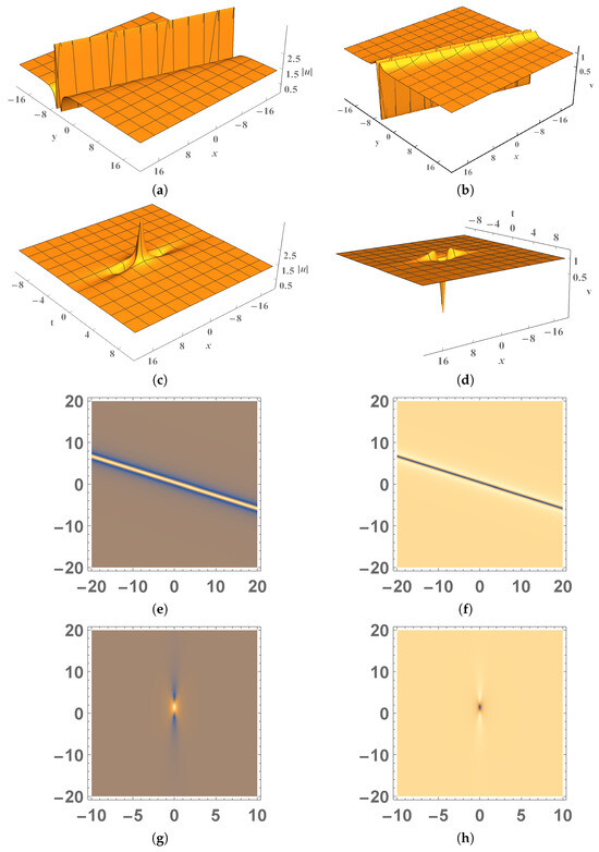
Figure 1.
The three-dimensional evolution plot (a–d) and density plot (e–h) of the fundamental rational solution with : (a,e) ; (b,f) ; (c,g) ; (d,h) .
From Figure 1a,b, it can be seen that and v both possess abnormal height, satisfying the characteristic of rogue waves. Meanwhile, it is obvious that, as , the solution uniformly approaches the constant background and the solution v uniformly approaches the constant background 1 everywhere in the plane. It is interesting to note that rogue wave v is a dark rogue wave, which is different from a bright rogue wave u. Because is constant, the figure illustrates that these rogue waves are linear. In Figure 1c,d, we find that there is only one peak in each figure, which is the characteristic of the fundamental rational solution.
4.2. Multi-Rogue Wave Solution
One subclass of nonfundamental rogue waves consists of multi-rogue waves, which can be obtained when taking , in the rational solution (10) with real values of . These rogue wave solutions describe the interaction of N individual fundamental rogue waves. In the near field of the plane, these line rogue waves intersect and are no longer lines, allowing interesting curvy wave patterns to appear. However, the solution consists of N rogue waves with separate lines in the far field.
To present these multi-rogue waves, we first consider the case with . In this case, the f and g functions of the solutions can be obtained from (10) as follows:
Similarly, with Equation (10), we can select parameters to illustrate graphics, as in Figure 2 and Figure 3.
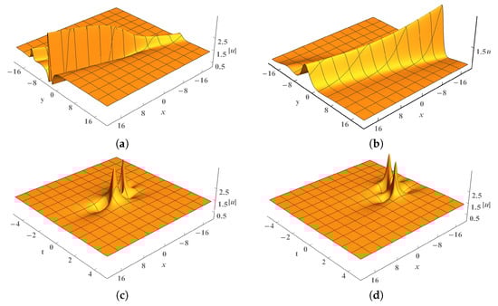
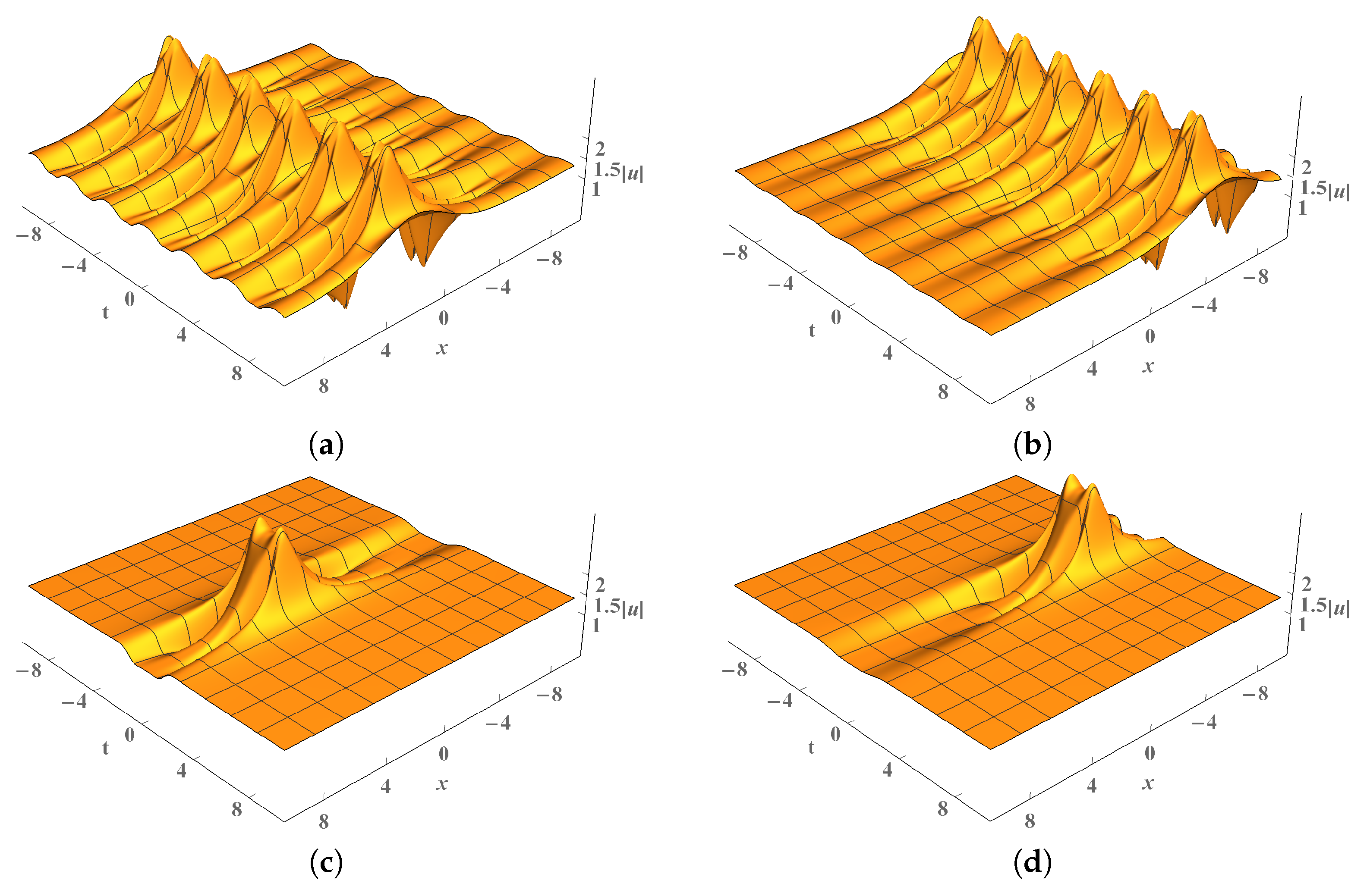
Figure 2.
Three-dimensional evolution plot of the multi-rogue rational solution with : (a) ; (b) ; (c) ; (d) .
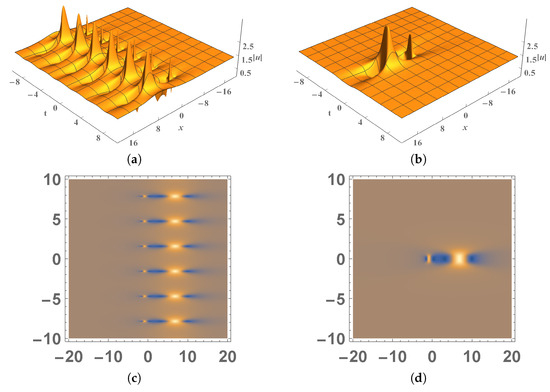
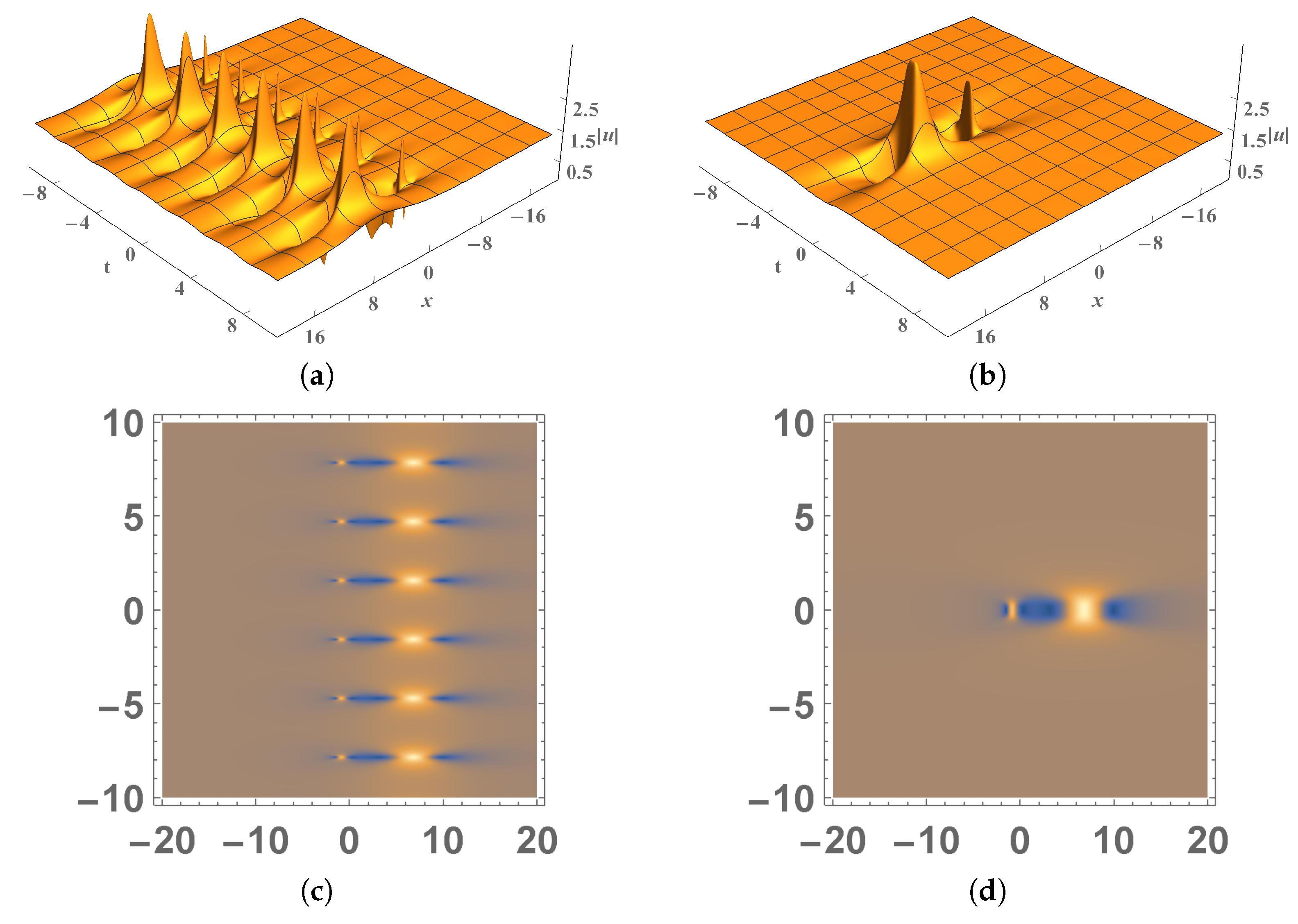
Figure 3.
The three-dimensional evolution plot (a,b) and density plot (c,d) of the multi-rogue wave solution with : (a,c) ; (c,d) .
From Figure 2a,b, it is clear that as the time t increases, there is a large change in the shape of . At the same time, the rogue waves converges and the spatial range involved becomes smaller. The process consists of the rogue waves commencing along a single straight path, gaining speed until they encounter a head-on collision, becoming dispersed and rotated, and ultimately diverging from each other in some direction [29]. From Figure 2c,d, it can be observed that there are two peaks of , which meets the characteristic of . Meanwhile, the shape of the peak does not change significantly with increasing y, but the position of the spatiotemporal coordinates changes greatly.
In addition, it can be seen that the amplitude and propagation direction of rogue wave change greatly with the parameter.
4.3. Higher-Order Rogue Wave Solution
Another subclass of nonfundamental rogue waves consists of higher-order rogue waves, which are obtained when we take , in the rational solution (10) with a real value of . For instance, if , we obtain a second rogue wave solutions as follows:
The expression for is shown in Equation (51). Combined with Equation (10), we can now select the parameters and obtain the graphical illustrations in Figure 4 and Figure 5.

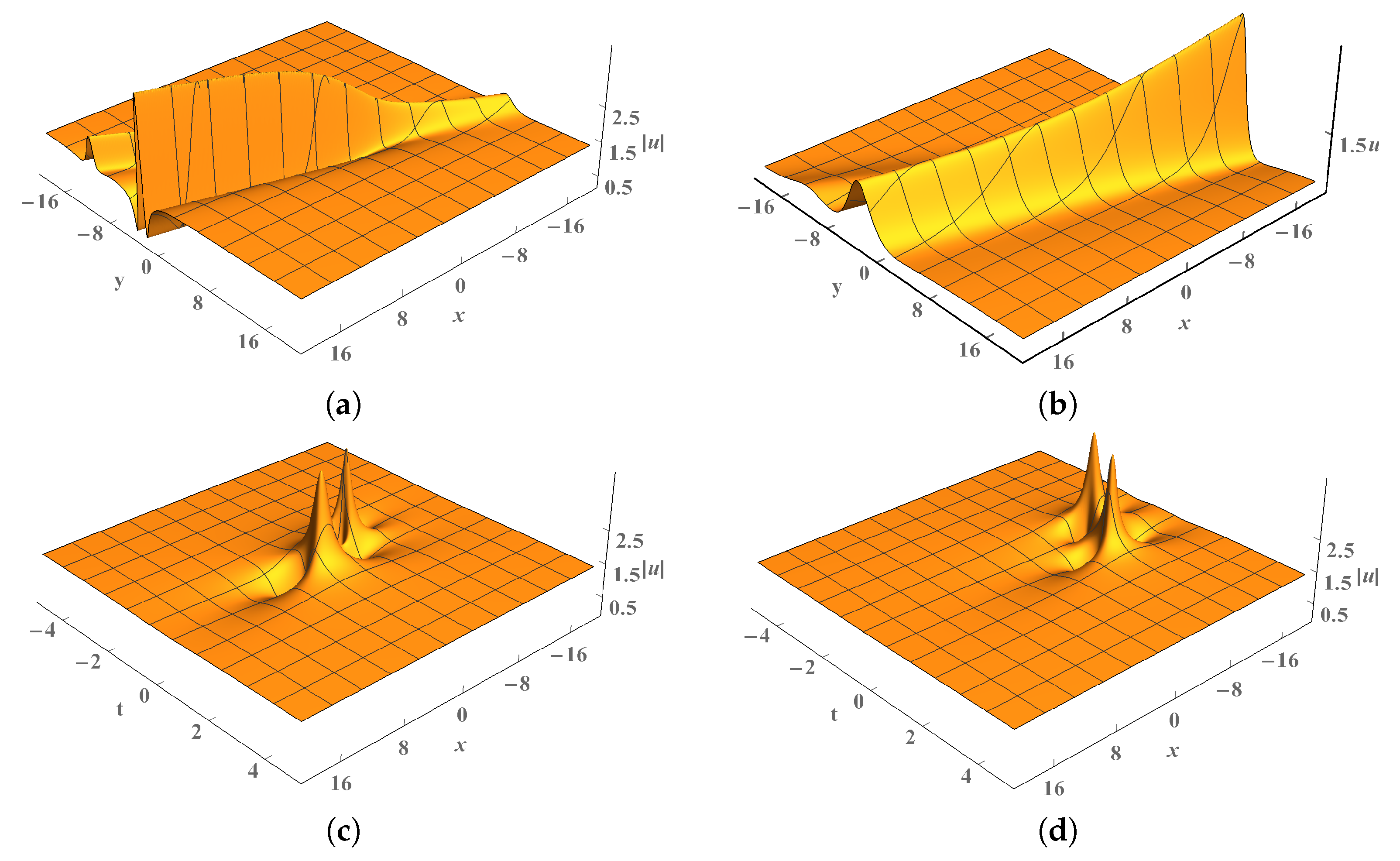
Figure 4.
Three-dimensional evolution plot of the higher-order rogue wave solution with : (a) ; (b) ; (c) ; (d) .
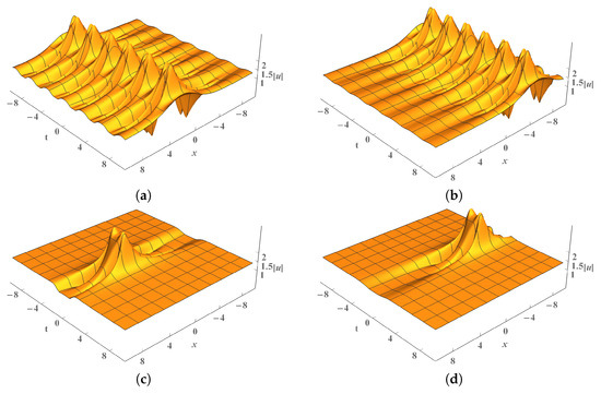
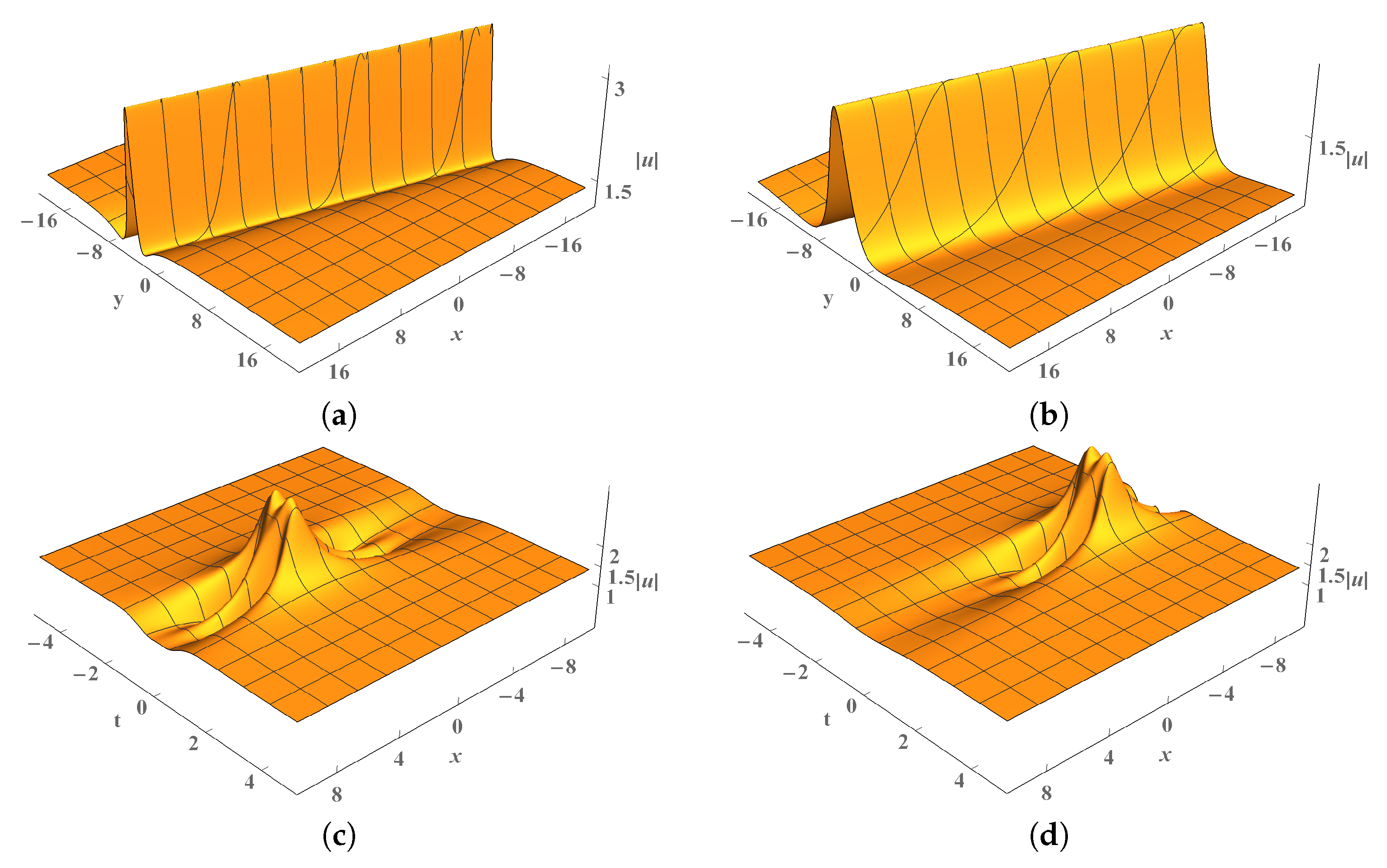
Figure 5.
Three-dimensional evolution plot of the higher-order rogue wave solution with : (a) ; (b) ; (c) ; (d) .
As shown in Figure 4a,b, when the time changes, the rogue waves converge; however, the amplitude of the waves does not change markedly. Observing Figure 4c to Figure 5d and taking different variable coefficients and y values, it can be seen that the shape of the higher-order rogue wave is more complex; indeed, it is the same as that of the multi-rogue wave in that the shape of the peak does not change significantly with changing y, but the spatiotemporal position changes greatly.
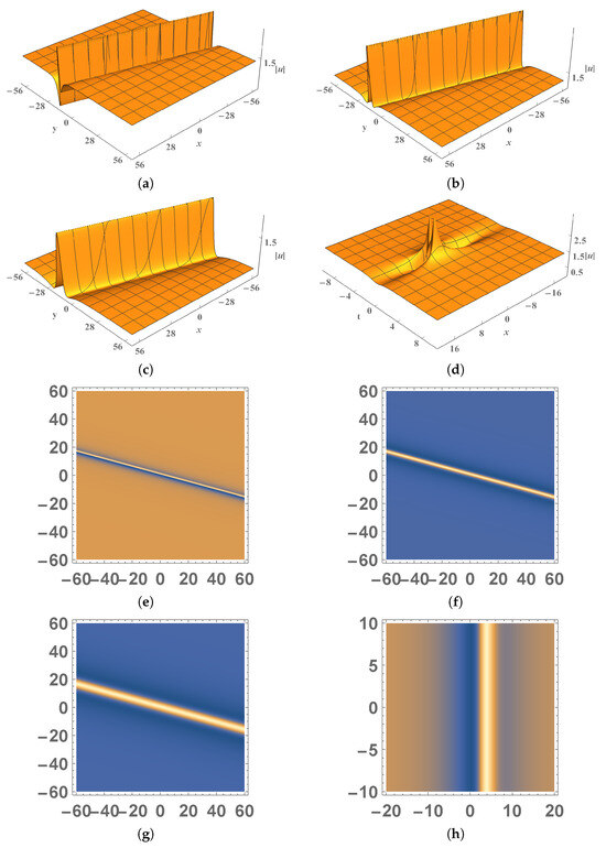
Figure 6.
The three-dimensional evolution plot (a–d) and density plot (e–h) of the third-order rogue wave solution with : (a,e) ; (b,f) ; (c,g) ; (d,h) .
5. Conclusions
The variable-coefficient DS equation is important in modeling ocean waves as well as ultra-relativistic degenerate dense plasmas Bose–Einstein condensates, and in some other nonlinear contexts where inhomogeneities of the media and nonuniformities of the boundaries need to be taken into consideration. In this paper, we have investigated a variable-coefficient Davey–Stewartson system, namely, a (2 + 1)-dimensional wave packet on the surface of a liquid of finite depth, via symbolic computation.
With respect to , e.g., the amplitude of a surface wave packet, and , e.g., the velocity potential of the mean flow interacting with the surface wave, the Painlevé integrability has been tested with the Weiss, Tabor, and Carnevale (WTC) method, proving that System (3) has Painlevé properties with certain parameter restrains. In addition, the bilinear forms of System (3) have been provided by means of variable transformation. Based on the obtained bilinear forms, rational solutions have been obtained by taking certain parameter restraints and deriving the corresponding rogue wave solutions. Furthermore, we have classified different kinds of rogue wave solutions and presented graphical illustrations illustrating their physical properties.
In comparison to other published results, in [23] rogue wave solutions of Equation (1) were derived in terms of the determinant and different types of rogue wave solutions were classified. In this paper, a variable-coefficient Davey–Stewartson (vcDS) Equation (3) is investigated, which can describe situations more realistically than Equation (1) when considering inhomogeneous media and nonuniform boundaries. Furthermore, [29] constructed higher-order lumps, k-order localized rogue waves, and line rogue waves on a -line soliton background. This direction is more concerned with soliton interactions, which may enlighten us in our following research.
The variable-coefficient constraints for the DS system (3) investigated this paper are strong; weaker coefficient constraints and a wider range of rational and rogue wave solutions are yet to be explored. In the future, we hope to improve the conditions and conclusions of the results presented in this paper in order to obtain rogue wave solutions with a wider form.
Author Contributions
Conceptualization, H.C. and G.W.; methodology, H.C. and Y.X.; computation, H.C. and Y.X.; resources, H.C. and G.W.; writing—original draft preparation, H.C. and Y.S.; visualization, H.C. and Y.X.; validation, G.W.; supervision, G.W.; project administration, G.W.; formal analysis, H.C. and Y.S.; writing—review and editing, H.C. and Y.S. All authors have read and agreed to the published version of the manuscript.
Funding
This research received no external funding.
Data Availability Statement
The data presented in this study are available on request from the corresponding author due to privacy reasons.
Acknowledgments
We would like to thank the editors and reviewers for their timely and valuable comments and suggestions.
Conflicts of Interest
The authors declare no conflicts of interest.
References
- Alqahtani, R.T.; Kaplan, M. Analyzing Soliton Solutions of the Extended (3 + 1)-Dimensional Sakovich Equation. Mathematics 2024, 12, 720. [Google Scholar] [CrossRef]
- Evans, L.C. Partial Differential Equations; American Mathematical Society: Providence, RI, USA, 2010. [Google Scholar]
- Pinelas, S.; Selvam, A.; Sabarinathan, S. Ulam–Hyers stability of linear differential equation with general transform. Symmetry 2023, 15, 2023. [Google Scholar] [CrossRef]
- Selvam, A.; Sabarinathan, S.; Nisar, K.S.; Ravichandran, C.; Senthil Kumar, B.V. Results on Ulam-type stability of linear differential equation with integral transform. Math. Method Appl. Sci. 2024, 47, 2311–2323. [Google Scholar] [CrossRef]
- Sivashankar, M.; Sabarinathan, S.; Govindan, V.; Fernandez-Gamiz, U.; Noeiaghdam, S. Stability analysis of COVID-19 outbreak using Caputo-Fabrizio fractional differential equation. AIMS Math. 2023, 8, 2720–2735. [Google Scholar] [CrossRef]
- Selvam, A.; Sabarinathan, S.; Senthil Kumar, B.V.; Byeon, H.; Guedri, K.; Eldin, S.M.; Khan, M.I.; Govindan, V. Ulam-Hyers stability of tuberculosis and COVID-19 co-infection model under Atangana-Baleanu fractal-fractional operator. Sci. Rep. 2023, 13, 9012. [Google Scholar] [CrossRef] [PubMed]
- Miah, M.M.; Seadawy, A.R.; Ali, H.S.; Akbar, M. Further investigations to extract abundant new exact traveling wave solutions of some NLEEs. J. Ocean Eng. Sci. 2019, 4, 387–394. [Google Scholar] [CrossRef]
- Barman, H.K.; Roy, R.; Mahmud, F.; Akbar, M.; Osman, M. Harmonizing wave solutions to the Fokas-Lenells model through the Kudryashov method. Optik 2021, 229, 166294. [Google Scholar] [CrossRef]
- Gao, X.Y. Two-layer-liquid and lattice considerations through a (3 + 1)-dimensional generalized Yu-Toda-Sasa-Fukuyama system. Appl. Math. Lett. 2024, 152, 109018. [Google Scholar] [CrossRef]
- Gao, X.Y. Auto-Bäcklund transformation with the solitons and similarity reductions for a generalized nonlinear shallow water wave equation. Qual. Theory Dyn. Syst. 2024, 23, 181. [Google Scholar] [CrossRef]
- Gao, X.Y. In the shallow water: Auto-Bäcklund, hetero-Bäcklund and scaling transformations via a (2+1)-dimensional generalized Broer-Kaup system. Qual. Theory Dyn. Syst. 2024, 23, 184. [Google Scholar] [CrossRef]
- Dong, H.N.; Zha, Q.L. Hybrid rogue wave and breather solutions for the nonlinear coupled dispersionless evolution equations. Wave Motion 2024, 125, 103259. [Google Scholar] [CrossRef]
- Zhang, H.W.; Zong, J.; Tian, G.; Wei, G.M. Analysis of High-Order Bright–Dark Rogue Waves in (2+1)-D Variable-Coefficient Zakharov Equation via Self-Similar and Darboux Transformations. Mathematics 2024, 12, 1359. [Google Scholar] [CrossRef]
- Smith, R. Giant waves. Fluid Mech. 1976, 77, 417–431. [Google Scholar] [CrossRef]
- Heller, E.J. Bound-state eigenfunctions of classically chaotic hamiltonian systems: Scars of periodic orbits. Phys. Rev. Lett. 1984, 53, 1515. [Google Scholar] [CrossRef]
- Arranz, F.J.; Borondo, F.; Benito, R.M. Scar formation at the edgeof the chaotic region. Phys. Rev. Lett. 1998, 80, 944–947. [Google Scholar] [CrossRef]
- Gao, X.Y. Oceanic shallow-water investigations on a generalized Whitham-Broer-Kaup-Boussinesq-Kupershmidt system. Phys. Fluids 2023, 35, 127106. [Google Scholar] [CrossRef]
- Osborne, A. Rogue waves: Classification, measurement and data analysis, and hyperfast numerical modeling. Eur. Phys. J. Spec. Top. 2010, 185, 225–245. [Google Scholar] [CrossRef]
- Yan, Z. Vector financial rogue waves. Phys. Lett. A 2011, 375, 4274–4279. [Google Scholar] [CrossRef]
- Ling, L.M.; Su, H.J. Rogue waves and their patterns for the coupled Fokas–Lenells equations. Phys. D Nonlinear Phenom. 2024, 461, 134111. [Google Scholar] [CrossRef]
- Davey, A.; Stewartson, K. On three-dimensional packets of surface waves. Proc. R. Soc. Lond. A 1974, 338, 101–110. [Google Scholar]
- Matveev, V.B.; Salle, M.A. Darboux Transformations and Solitons; Springer: Berlin, Germany, 1991. [Google Scholar]
- Ohta, Y.; Yang, J.K. Rogue waves in the Davey-Stewarton I equation. Phys. Rev. E 2012, 86, 036604. [Google Scholar] [CrossRef] [PubMed]
- Zhou, H.P.; Tian, B.; Mo, H.X.; Li, M.; Wang, P. Bäcklund transformation, Lax pair and solitons of the (2 + 1)-dimensional Davey-Stewartsonlike equations with variable coefficients for the electrostatic wave packets. J. Nonlinear Math. Phys. 2013, 20, 94–105. [Google Scholar] [CrossRef]
- Ablowitz, M.J.; Segur, H. On the transition from two-dimensional to three-dimensional water waves. Stud. Appl. Math. 2000, 104, 91–127. [Google Scholar]
- Zhang, Y.P.; Wang, J.Y.; Wei, G.M. The Painlevé property, Bäcklund transformation, Lax pair and new analytic solutions of a variable-coefficient KdV equation from fluids and plasmas. Phys. Scr. 2015, 90, 065203. [Google Scholar]
- Tajiri, M.; Arai, T. Growing-and-decaying mode solution to the Davey-Stewartson equation. Phys. Rev. E 1999, 60, 2297. [Google Scholar] [CrossRef] [PubMed]
- Guo, L.; He, J.; Mihalache, D. Rational and semi-rational solutions to the asymmetric Nizhnik Novikov-Veselov system. J. Phys. A Math. Theor. 2021, 54, 095703. [Google Scholar] [CrossRef]
- Guo, L.J.; Chen, L.; Mihalache, D.; He, J.S. Dynamics of soliton interaction solutions of the Davey-Stewartson I equation. Phys. Rev. E 2022, 105, 014218. [Google Scholar] [CrossRef]
- Wei, G.M.; Lu, Y.L.; Xie, Y.Q.; Zheng, W.X. Lie symmetry analysis and conservation law of variable-coefficient Davey–Stewartson equation. Comput. Math. Appl. 2018, 75, 3420–3430. [Google Scholar] [CrossRef]
- Wang, R.J.; Huang, Y.C. Exact solutions and excitations for the Davey–Stewartson equations with nonlinear and gain terms. Eur. Phys. J. D 2010, 57, 395–401. [Google Scholar] [CrossRef]
- Wei, G.M.; Gao, Y.T.; Xv, T.; Meng, X.H.; Zhang, C.Y. Painlevé property and new analytic solutions for a variable-coefficient Kadomtsev-Petviashvili equation with symbolic computation. Chin. Phys. Lett. 2008, 25, 1599–1602. [Google Scholar]
- Srivastava, S.; Kumar, M. Nonclassical symmetries, optimal classification, and dynamical behavior of similarity solutions of (3 + 1)-dimensional Burgers equation. Chin. J. Phys. 2024, 89, 404–416. [Google Scholar] [CrossRef]
- Weiss, J.; Tabor, M.; Carnevale, G. Carnevale, The Painlevé property for partial dierential equations. J. Math. Phys. 1983, 24, 522–526. [Google Scholar] [CrossRef]
- Weiss, J.; Tabor, M.; Carnevale, G. The Painlevé property for partial differential equations II: Bäcklund transformation, Lax pairs, and the Schwarzian derivative. J. Math. Phys. 1983, 24, 1405–1413. [Google Scholar] [CrossRef]
- Xu, G.Q. A note on the Painlevé test for nonlinear variable-coefficient PDEs. Comput. Phys. Commun. 2009, 180, 1137–1144. [Google Scholar] [CrossRef]
- Hirota, R. The Direct Method in Soliton Theory; Cambridge University Press: Cambridge, UK, 2004. [Google Scholar]


Disclaimer/Publisher’s Note: The statements, opinions and data contained in all publications are solely those of the individual author(s) and contributor(s) and not of MDPI and/or the editor(s). MDPI and/or the editor(s) disclaim responsibility for any injury to people or property resulting from any ideas, methods, instructions or products referred to in the content. |
© 2024 by the authors. Licensee MDPI, Basel, Switzerland. This article is an open access article distributed under the terms and conditions of the Creative Commons Attribution (CC BY) license (https://creativecommons.org/licenses/by/4.0/).