Abstract
Three-wheeled omnidirectional mobile robots (TOMRs) are widely used to accomplish precise transportation tasks in narrow environments owing to their stability, flexible operation, and heavy loads. However, these robots are susceptible to slippage. For wheeled robots, almost all faults and slippage will directly affect the power consumption. Thus, using the energy consumption model data and encoder data in the healthy condition as a reference to diagnose robot slippage and other system faults is the main issue considered in this paper. We constructed an energy model for the TOMR and analyzed the factors that affect the power consumption in detail, such as the position of the gravity center. The study primarily focuses on the characteristic relationship between power consumption and speed when the robot experiences slippage or common faults, including control system faults. Finally, we present the use of a table-based artificial neural network (ANN) to indicate the type of fault by comparing the modeled data with the measured data. The experiments proved that the method is accurate and effective for diagnosing faults in TOMRs.
Keywords:
three-wheeled omnidirectional mobile robot (TOMR); energy consumption model; power measurement; fault diagnosis; power patterns MSC:
93C95
1. Introduction
The basic structure of a three-wheeled omnidirectional mobile robot (TOMR) consists of three omnidirectional wheels, symmetrically distributed at 120-degree intervals. The special structure of the omnidirectional wheels allows the robot to move in all directions [1]. This holonomicity makes it easier to control and plan the trajectory in complex and narrow places. Due to their high mobility, robots with this type of wheels are often used in industrial applications [2] and educational platforms [3]. Some studies have equipped omnidirectional-wheeled robots with additional mechanisms, such as robotic arms. This configuration not only gives full advantage to the flexibility and mobility of omnidirectional-wheel robots, but also dramatically increases the working space of manipulators such as robotic arms [4,5]. Unfortunately, although omnidirectional wheels offer high maneuverability, TOMRs are also more prone to slippage than standard wheels.
The omnidirectional-wheel robot’s slippage is caused by the friction between the omnidirectional wheel and the floor surface being too small to transfer all the force correctly. The torque provided by the motor to the wheels is only partly transformed into the motion of the vehicle, and the contact point between the wheels and the floor slips relative to the floor [6]. Han et al. pointed out that wheel slippage is the main source of position error in omnidirectional mobile robots [7]. In trajectory planning, it is common to rely on the odometer, which uses wheel encoder data as the direct estimate of displacement and velocity, but this approach usually requires assurance that the robot is in a no-slip condition. When the robot skids, odometer-based position estimation will quickly accumulate large errors, because relying solely on the encoder data from the wheels it is impossible to distinguish whether the wheels are rotating normally but slipping, or if the robot is moving normally. This results in significant errors in the robot’s position relative to the correct location during periodic position updates [8].
To avoid slipping, most self-driving cars in the industry use kinematic and dynamics models to plan vehicle trajectories and limit the speed and acceleration of the vehicle [9,10]. Nevertheless, this significantly increases the economic cost and is not very useful for omnidirectional mobile robots. If the robot slips, it can lead to unexpected and undesired behavior (such as colliding with an obstacle or drifting) and can complicate the prediction of robot motion by nearby personnel, which can be a serious safety hazard [11]. In summary, it is necessary to detect slippage of robots in real time, especially omnidirectional-wheel robots, which requires high-precision control to prevent serious damage.
The problem of wheel slip has been studied by many scholars. The easiest way to detect whether a robot is slipping or not is to use GPS signals, which will provide accurate position and speed information in open terrain [12,13,14]. Unfortunately, the GPS signal is not available in the presence of obscured environments and indoor environments [15]. Chang et al. [16] determine whether each drive wheel of an omnidirectional robot is faulty by comparing the magnitude of viscous friction coefficient with the residual value. Still, this approach requires solving for the magnitude of the coefficient of viscous friction for each wheel in real time, which is very difficult and dramatically increases the calculation cost. F. Gustafsson [17] proposed to compare the speed of the driven wheels with the speed of the non-driven wheels. By comparing the encoder data, wheel slip can be accurately estimated. But this approach is not applicable to all-wheel-drive robots such as omnidirectional-wheel robots.
For all-wheel-drive robots, Ojeda et al. [18] proposed to compare the redundant wheel encoder data with each other and their yaw gyroscope data as an indicator of wheel slip. However, this method does not estimate the degree of robot slippage and requires additional redundant encoders to be attached to the robot, which undoubtedly increases the cost of the robot [19]. Chris et al. [8] proposed an approach to fuse robot encoder data, inertial measurement unit (IMU) data, and dynamic robot models in an extended Kalman filter (EKF) to detect robot slips. This avoids the need to attach redundant encoders. The limitation of this method is that it can only detect longitudinal sliding along the direction of motion. In the presence of lateral forces, the wheels move at an angle with respect to the longitudinal wheel plane, resulting in lateral sliding, which is very common in omnidirectional-wheel robots. Ojeda et al. [20] also proposed a motor-current-based differential rotation estimator. Nevertheless, this technique requires accurate current measurements and terrain-specific parameter tuning, and the proposed tuning technique requires accurate absolute positioning devices or robots with at least four driving wheels. In addition, some studies have suggested introducing visual odometry (VO) data to estimate robot velocity and slip [21,22,23]. But according to the data provided by the authors, the VO error on short time scales is about 12% [24], which is beyond the maximum tolerable error range. In environments that lack distinctive features, such as smart factories, the performance of VO may be compromised.
However, the above-mentioned work has a common disadvantage, that although it is possible to determine to some extent whether the robot is slipping or not, it is not possible to discern the cause of the slippage [25]. The robot’s motor fault or control system fault can also lead to similar slippage, but these faults need to be dealt with differently. According to the study in [26], different faults of the robot will have different effects on the power consumption pattern of the robot, and this correspondence holds even during the acceleration and braking phases when the power consumption changes drastically.
In this paper, we compare the data from the energy consumption model with the data actually measured during the execution of the task to determine the causes of robot faults and take different actions. The energy model of a robot can provide a reference value for the robot’s power consumption. Therefore, an accurate energy consumption model is very significant for fault diagnosis. This study achieves fault detection and diagnosis of the TOMB by analyzing power consumption data under different fault conditions. This energy consumption modeling approach is similar to the energy-based maintenance (EBM) paradigm proposed by Orosnjak et al. [27], which aims to detect quasi-fault events by setting functional-productiveness thresholds to achieve cleaner production.
Morales et al. [28] modeled the energy consumption of a crawler robot in an outdoor scenario by both the power generated by the rigid terrain and the power provided by the electric motor. Wang et al. [29] studied the dynamics model of the robot mechanics as well as the model of the motors, and proposed a new kinetic model that takes into account all the main parameters. Liu and Sun [30] proposed an energy consumption model for a wheeled robot by considering the energy conversion of the robot and adding the energy to overcome the traction resistance and the energy converted into kinetic energy of the robot to the model. Then, the established model was added to the criterion of the A* algorithm to form the path with the lowest energy consumption to reach the destination. Xu et al. [31] proposed a method for modeling the energy consumption of industrial robots that avoids the need to directly measure various parameters inside the robots, which provides convenience for the application of energy consumption models. Thiago et al. [32] developed an adaptive motion controller for trajectory tracking of nonholonomic mobile robots under longitudinal and lateral slip, reducing additional energy consumption caused by improper control or environmental changes. Song et al. [33] developed an AI-based fault detection system for wiring harness manufacturing that employs regional selective data scaling (RSDS) to create synthetic abnormal data, enhancing the efficiency and accuracy of quality control processes without relying on actual defect data. Hendzel et al. [34] proposed an adaptive fuzzy control scheme that allows for online adjustment of control parameters, enabling real-time compensation for the nonlinear dynamic characteristics of mobile robots, thus enhancing the control accuracy and adaptability of the system. Li et al. [35] proposed a prescribed-time zero-error active disturbance rejection control strategy, innovatively designing a prescribed-time extended state observer (PTESO) for wheeled mobile robots subject to skidding and slipping. However, the requirement for high gain may lead to actuator limitations and numerical stability issues.
Jaramillo-Morales et al. [36,37] proposed an energy consumption model based on the dynamic parameters of the mobile robot and motor, which ensures that the model can accurately predict the required energy even if the robot carries different weights of payloads and performs different tasks. Wang et al. [38] proposed an energy consumption model for omnidirectional-wheel robots that is used to find optimal energy trajectories. Xie et al. [39,40] developed an energy consumption model for Mecanum wheel robots and applied this model to a local trajectory planner based on an extended dynamic window. The local trajectory planner was proven to be effective in reducing the energy consumption of the robot. Furthermore, Hou et al. [41] predict the energy consumption of omnidirectional-wheel robots with an accuracy of about 90%. In this work, we developed an energy model for the energy consumption of TOMRs during omnidirectional movements, which is based on a comprehensive analysis of the robot’s kinematics, dynamics, and energy flow.
The main contributions of this paper are threefold:
- (1)
- A comprehensive energy model for a three-wheeled omnidirectional robot has been developed, analyzing various factors that affect power consumption, including the position of the center of gravity.
- (2)
- The relationship between power consumption curves and robot encoder speed as well as fault characteristics is presented.
- (3)
- Using power consumption as the main basis, a method has been developed to distinguish the types of actual failures that might take place in the robot during operation.
The paper is presented as follows. Section 2 introduces the energy consumption model of the TOMR and analyzes the factors affecting the energy consumption in detail. Section 3 presents the impact of three typical faults that may occur in the robot in its energy consumption patterns. Section 4 presents how to use neural networks, energy consumption models, and energy consumption measurements for fault diagnosis. Section 5 presents the conclusions after the analysis of the experimental results.
2. Energy Modeling
Kim et al. [42] conducted dynamic modeling and applied optimal control theory to TOMR robots, achieving reduced energy consumption by optimizing trajectory planning and control. Similar to Kim’s approach, we also decompose the overall energy consumption of the robot into several subsystems: the motion system, control system, and sensor system. The energy consumption of the robot, , can be expressed as
The energy consumption of the robot is mainly related to the motion environment and some parameters of the robot itself. The energy consumption of the motion system is the largest among the three subsystems, and the motion system is also the most influenced by the environment. After measuring and analyzing the energy consumption’s relationships with the other systems of the robot and the motion system, it is found that the energy consumption of other systems of the robot is related to the energy consumption of the motion system of the robot, and the energy consumption between each system can be related by a physical quantity v of the robot.
2.1. Motion System
The robot motion system is the system that accounts for the most significant proportion of the robot’s energy consumption, and it is also the most crucial system in the robot. The energy consumption of the robot motion system mainly comes from the consumption of motors during motion, and we can express the energy consumption of the motion system as follows:
where is the energy consumed by the robot motion system; is the energy consumed by the robot motion system during standby; and is the energy consumed by the robot motion system during running.
where is the power consumed by the motion system in standby mode, which is a constant for a deterministic motion system and can be directly measured by power measurement software.
According to the conservation of energy consumption, the energy output of the robot is the same as the energy consumed by each part of the robot. Thus, based on the energy consumption of each component of the omnidirectional-wheel robot during motion, we can roughly categorize the robot’s energy consumption in the motion system into five parts. The energy consumed by the robot during operation, denoted as , can be described as follows:
where is the kinetic energy added by the robot; is the energy dissipated in the form of thermal energy during the robot’s motion; is the energy consumed by the robot during motion due to friction; is the energy consumed by the robot during the motion to overcome the iron consumption of the motor, which is mainly the energy consumed by the robot during the motion to overcome the hysteresis loss; and is the energy consumed by the mechanical dissipation of the motion system.
- (1)
- The increased kinetic energy of the robot, denoted as , can be expressed as follows:where M is the robot’s mass, and v is the real-time speed of the robot. The increase in kinetic energy is only related to two variables, one is the mass of the robot, and the other is the speed of the robot. In the process of movement, the robot motor can realize the mutual conversion of kinetic energy and electrical energy. Testing reveals that during the acceleration phase the robot’s electrical energy is converted into kinetic energy. Conversely, during the deceleration phase, except in cases of emergency stopping, kinetic energy is often converted back into electrical energy.
- (2)
- The thermal energy dissipation of the robot, denoted as , can be expressed as follows:where and are the heat time parameters of the motors; is the heat torque parameter of the motors; is the heat constant of the robot, which is related to the quality of the robot itself; and is the heat time parameter of the robot.
- (3)
- The frictional energy dissipation of the robot, denoted as , can be expressed as follows:where represents the coefficient of friction specific to each wheel of the robot; is the normal force experienced by each wheel; and represents the angle between the robot’s forward direction and its positive direction.The energy consumed by the robot’s motion due to friction can be divided into two primary components: The first component is the energy consumed by the friction between the omnidirectional wheel and the ground during movement. This energy consumption depends on the robot’s speed and the angle , which is the angle between the robot’s forward direction and its positive direction. Secondly, because of the special structure of the omnidirectional wheel and the omnidirectional-wheel robot, the TORM relies on the frictional force in each direction to cancel and synthesize each other to form the combined force in any direction during motion, so it is inevitable that the frictional forces between each omnidirectional wheel will cancel each other during the motion, which is another part of the energy consumed by the frictional force.
- (4)
- The energy consumed by the robot during motion to overcome the iron consumption of the motor, denoted as , can be expressed as follows:The hysteresis loss in the robot’s motor is primarily associated with the robot’s speed and acceleration. During the acceleration phase of movement, the motor needs to increase its magnetic field to boost its speed. This enhancement requires energy to build the magnetic field. Consequently, the faster the robot’s speed and the greater its acceleration, the more stress is placed on the motor, leading to higher hysteresis losses.
- (5)
- The mechanical loss of the robot, denoted as , can be expressed as follows:The mechanical loss of the robot primarily stems from the energy dissipation caused by the friction between its mechanical structures during operation. This loss is significantly influenced by the robot’s mass and center of gravity during movement. Additionally, mechanical losses are closely linked to the speed of each drive wheel and the force exerted on each wheel. Higher pressures on the drive wheels, coupled with faster speeds, increase the stress on the mechanical structure, leading to greater mechanical losses. Furthermore, the torque output of the drive wheels is strongly correlated with the mechanical losses of the robot. Higher torque outputs require the robot to use more power to perform tasks, consequently increasing mechanical losses.
2.2. Sensor System
The power consumption of the sensor system, denoted as , can be expressed as follows:
where is the total power consumption of the sensor system and is the real-time power of one sensor in the robot sensor system. The power consumption of the sensor system varies greatly depending on the type of sensor and the detection frequency. The sensing system of a robot often consists of multiple sensors, each with different amounts of data, and the sensing frequency of the sensors varies at different speeds, so the power consumption of the robot’s sensing system needs to be analyzed and modeled. For the sensor sensing frequency, we use to represent the sensing frequency of different sensors; for the camera, the sensing frequency represents the number of frames per second of the camera; for the infrared laser sensor, it is the range frequency.
Therefore, for the sensor system, the power consumption is mainly related to the speed of the robot and the setting of the acquisition frequency. In the process of setting the sensor system of the robot, a margin of about 10–20% is reserved in the process of setting the parameters of the sensor system in order to ensure the needs of the robot for the sensors and the needs of safety, so as to prevent the occurrence of unexpected situations during the movement.
2.3. Control System
The power consumption of the control system is mainly related to the state of the robot and the settings of the sensor system. The changes in the robot’s motion state require the control system to calculate and estimate the current motion state and send the corresponding control signals for the robot to reach the set motion state. So, the energy consumption of the control system increases accordingly. Meanwhile, for the sensor system, the robot’s sensor system needs to keep sending the detected signals to the control system, and the control system needs to keep processing the signals sent by the sensor system to determine the current state of the robot, so the energy consumption of the control system can be expressed as Equation (11):
where represents the power consumption of the robot while in standby mode. Since the power consumption in this state is relatively stable, it can be expressed as an integral of over time; represents the power consumed under specific dynamic conditions, incorporating velocity (v), changes in velocity (), sensor activity factors (), and their proportionate impact relative to maximum velocity (); represents the energy consumption of the robot control system during stable operation phases, incorporating the power consumption of each component (), time-dependent power adjustment (), and standby power (). and are the time parameters of the robot control system, which are used to express the relationship between the power consumption of the robot control system and the running time of the robot control system.
For the robot control system, the longer the robot’s running time, the higher the energy consumption of the control system. This relationship reflects the cumulative impact of sustained operations on power usage. and characterize the data parameters of the robot control system. A large part of the power consumption of the control system comes from the processing of the data of the sensing system and the sending of the corresponding control commands to the motion system. The power consumption of the robot control system has a lot to do with the number and type of sensors of the robot, because the more complex the sensor type is, the more data the robot needs to process. For the same function, we can choose lidar or a depth camera, but compared to Lidar the power consumption of the depth camera is much higher.
2.4. The Effect of Robot Operation Angle on Power Consumption
For omnidirectional-wheel robots, because omnidirectional movement can be achieved, the angle between the direction of motion and the robot’s orientation can directly affect the power consumption. The power consumption is lowest when the angle between the robot’s direction of motion and the robot’s orientation is 0 degrees and highest when the robot’s direction of motion is 30 degrees. However, the highest power consumption is when the robot is most complex to control and when the robot has the highest motion capability. Therefore, it is necessary to choose the robot’s motion angle during robot movement to ensure both the principle of minimum robot power consumption and accurate robot control. For the direction of motion and the robot’s orientation angle mainly affect the frictional energy loss of the robot. This is because the wheels consume different amounts of energy to offset each other at different angles. The effect of friction loss is mainly reflected in the change in the friction factor.
The relationship between the friction force and the running angle of the robot can be expressed as
The influence of the angle between the direction of motion and the positive direction on the robot’s energy consumption is mainly focused on the energy consumed by the frictional forces between the drive wheels that offset each other. So, the overall friction parameters are different when the robot is moving at different angles. Due to the three wheels of the TOMR showing a symmetric distribution of 120 degrees, the power consumption of the omnidirectional-wheel robot shows a symmetric distribution of 60 degrees. The power consumption of the robot has a great relationship with the locomotion ability. The angle between the motion direction and the robot’s positive direction increases the energy consumption of the robot, but to a certain extent, it increases the robot’s locomotion ability. We modeled the relationship between the direction of motion and the climbing angle, and the modeling relationship can be represented in Equation (13):
After modeling, owing to the special mechanical structure of the TOMR, the effect of the angle between the direction of robot motion and the positive direction on the kinematic capability is symmetrically distributed at 30 degrees. Within the 30-degree range, the bigger the angle, the greater the overall friction coefficient of the robot and the greater the robot’s kinematic capability.
2.5. The Effect of Displacement of the Mass Center on Power Consumption
The mass center of the robot has a significant impact on power consumption. For a robot, we cannot guarantee that the mass center always coincides with the geometric center. When the center of mass of the robot is displaced considerably, the power consumption will change significantly.
Figure 1 shows the displacement of the center of mass of the robot with respect to the geometric center. (a) simply illustrates four different positions of the center of mass, shown in the four subfigures with shaded areas representing the center of mass locations. These varying positions of the center of mass affect the robot’s motion performance and energy consumption at different movement angles. (b) illustrates the position of the center of mass O and its relationship with the geometric center. The red coordinate axes in the figure represent the robot’s own coordinate system and . By using the parameters and , the position of the center of mass and its impact on the robot can be described more intuitively. Owing to the special structure of the TOMR, we used a form similar to polar coordinates to represent the displacement of the mass center with respect to the geometric center. That is, the distance between the mass center and the geometric center as well as the angle between the line connecting the center of mass and the geometric center and the positive direction of the robot .
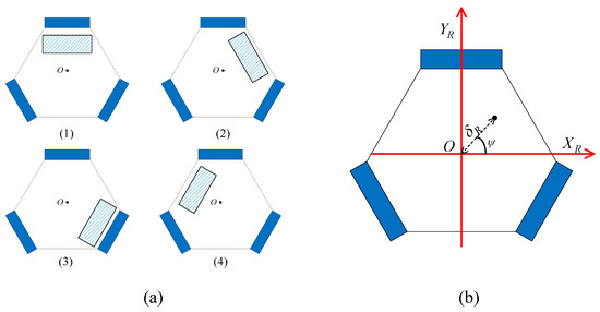
Figure 1.
Schematic diagram of the center of gravity and center position of the robot: (a) Robot with four different centers of gravity: (1) center of gravity located at the top center of the robot, (2) center of gravity located at the top right of the robot, (3) center of gravity located at the bottom right of the robot, (4) center of gravity located at the top left of the robot; (b) the position of the center of gravity.
The influence of the displacement of the mass center on the power consumption is mainly reflected in the friction factors and , as well as the positive pressure applied to each of the driving wheels. The first is the effect on the friction coefficient of the robot.
The above equation shows that the displacement of the mass center has a tremendous effect on the robot’s friction, mainly by affecting the friction factor, and thus, the overall frictional power consumption of the robot. Where L represents the length of the robot’s sides (see in Figure 2), represents the length from the center of the robot to each side of the robot, and finally, is the straight-line distance from the center of the robot to the drive wheels.

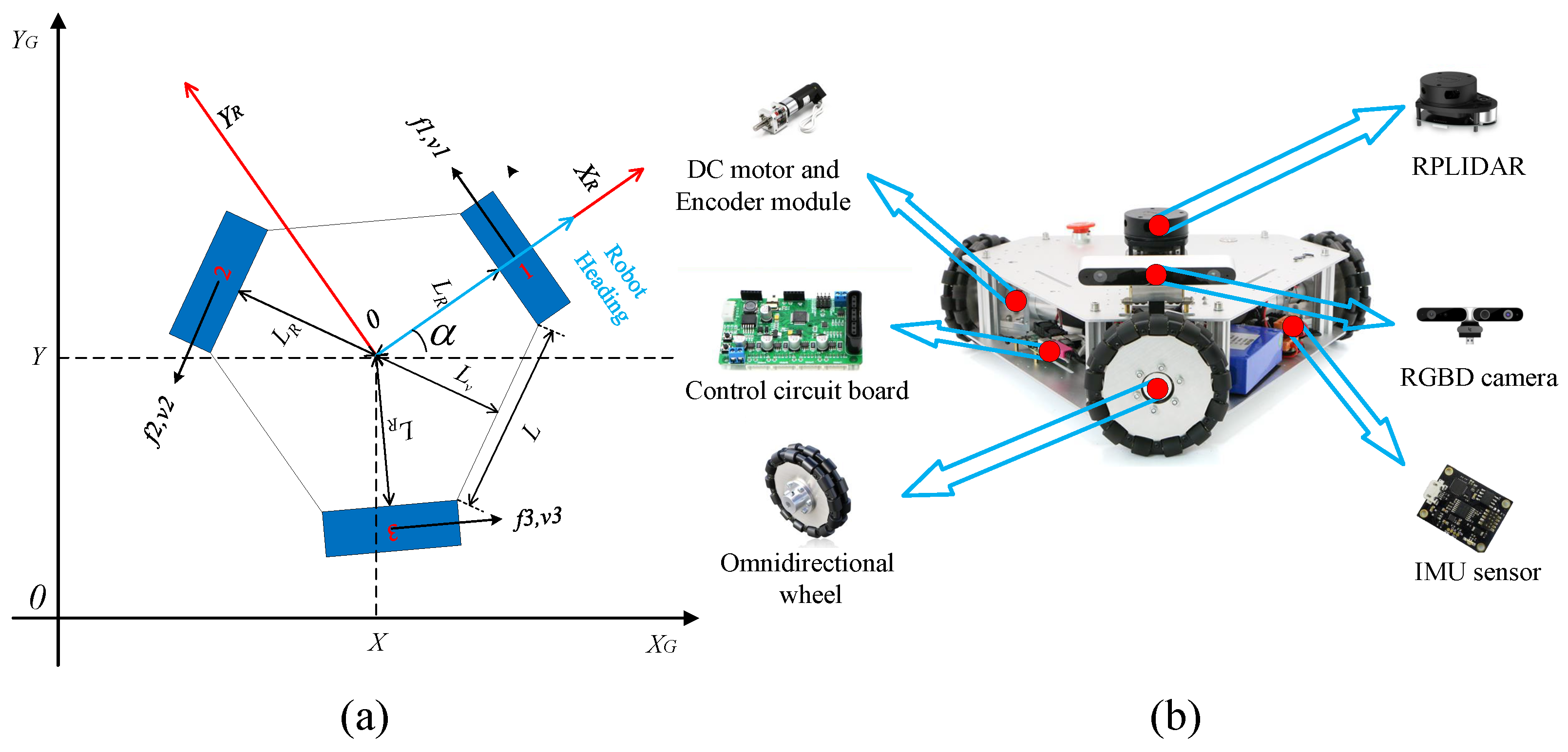
Figure 2.
Schematic diagram of the TOMR: (a) Schematic diagram of robot structure; (b) robot physical analysis diagram.
The second is the effect on the positive pressure on each of the drive wheels:
Equation (17) shows the effect of the displacement of the mass center on the positive pressure of each driving wheel of the robot, where represents the positive pressure on the corresponding drive wheel of the robot and represents the angle between the corresponding drive wheel and the center of gravity of the robot.
2.6. Results of Power Consumption Modeling and Speed Modeling
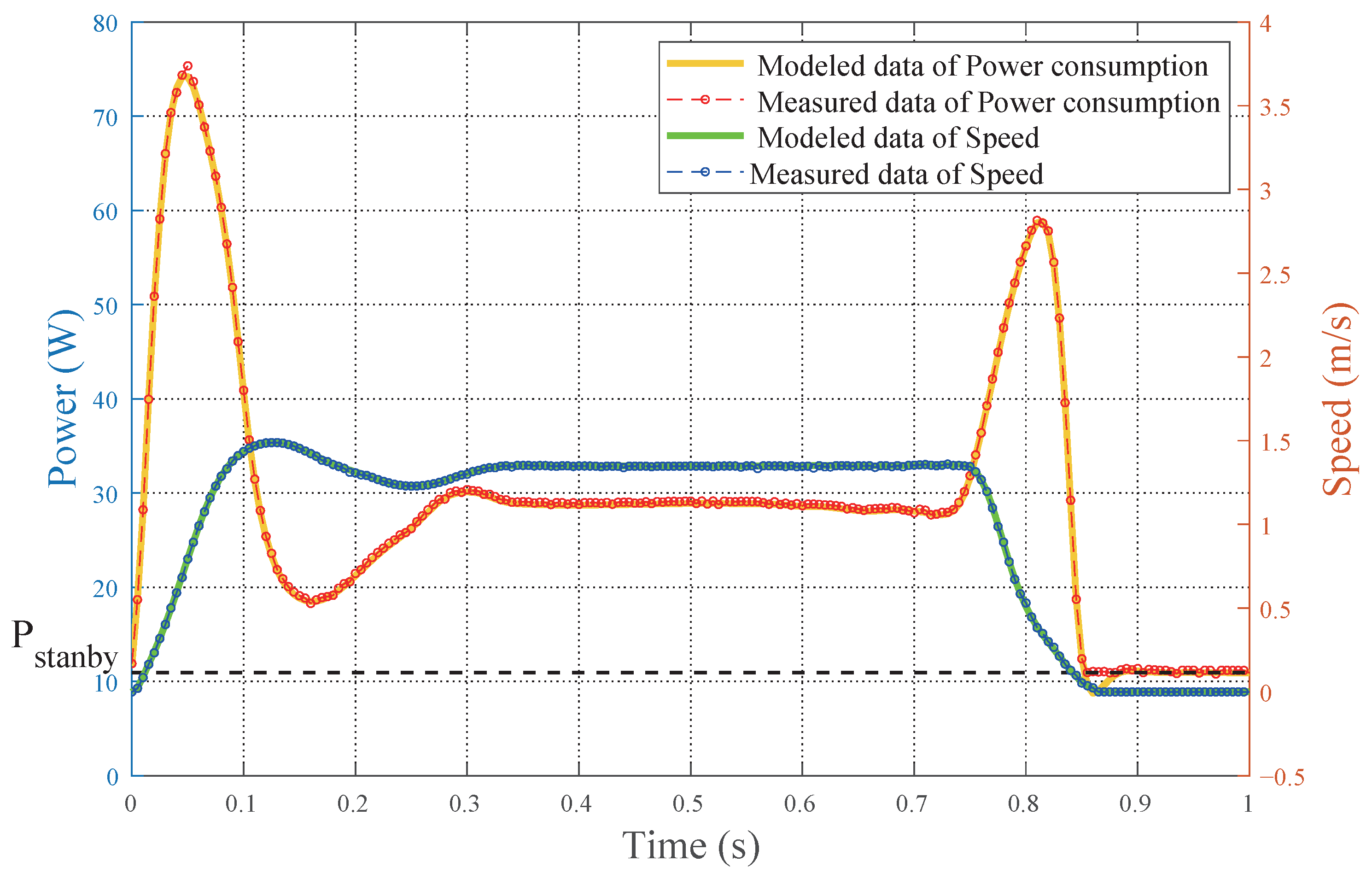
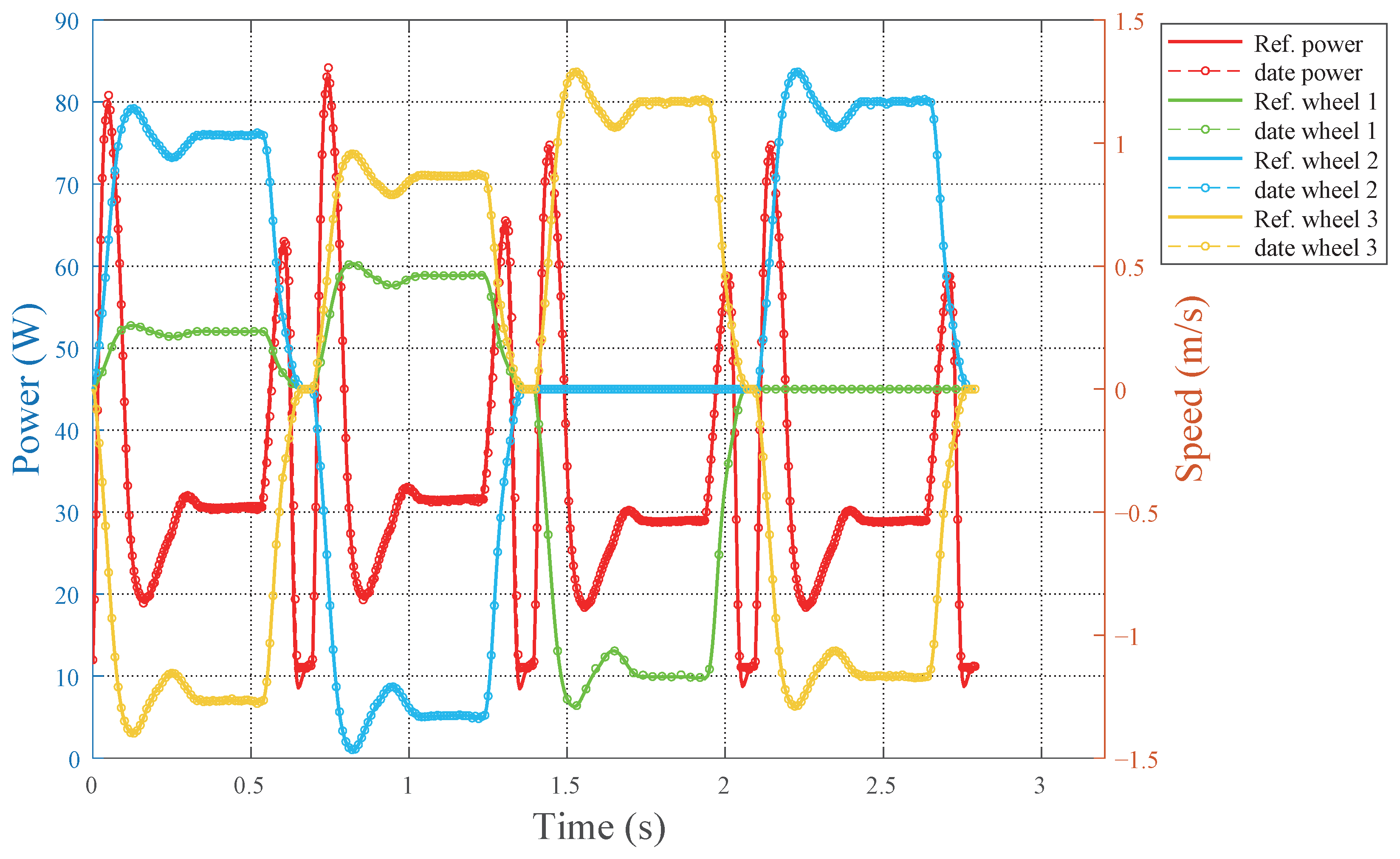
Figure 3 shows the results of the power consumption modeling and speed modeling. According to the previous theory, before power consumption modeling, we need to model the speed first, because speed is not only the basis of power consumption modeling, but also the bridge to link the power consumption relationship of each subsystem. The modeling results show the relationship between the overall robot speed and power consumption during the movement in the positive direction along the Y-axis.
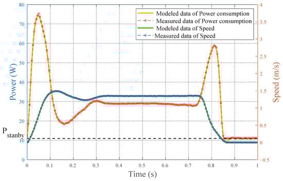
Figure 3.
Comparison of modeled/measured data for speed and power consumption.
It can be seen that the overall energy consumption and speed modeling is relatively successful. With the exception of the two phases where the energy consumption changes very drastically, the start phase and the braking phase, there is a slight difference between the modeled power consumption values and the actual measured values of the robot. The modeled values of power consumption and speed are in good agreement with the actual measured values at all other times.
In the beginning, the speed starts to increase because the acceleration is very high and the motor needs to establish the magnetic field, which consumes energy, so the power consumption of the robot changes very drastically at this time. With the proportional–integral–derivative (PID) control, the speed and power consumption fluctuate to a certain extent, and the fluctuation of power consumption disappears when the speed gradually stabilizes to the pre-set value. During the deceleration phase, the changes in power and speed are relatively slow. However, due to the PID control, when the speed decreases to zero, the PID controller may temporarily reduce the power output excessively in an effort to quickly reach the target speed (zero). This can cause the instantaneous power consumption to fall below the standby power level. This situation is usually temporary, and once the speed stabilizes, the power consumption returns to normal levels.
To verify the effect of the offset of the center of gravity on the power consumption, for the triangular structure of the omnidirectional-wheel robot, using a method similar to polar coordinates, the offset of the robot’s center of gravity with respect to the robot’s center is represented by two variables, which are the angle between the line connecting the center of gravity of the robot to the center and the positive direction of the robot, and the distance from the center of gravity to the center.
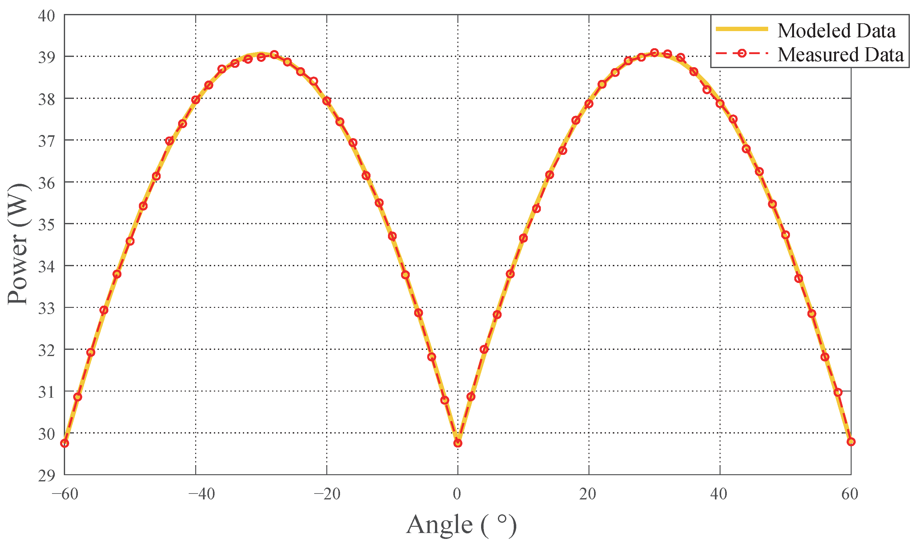
Figure 4 shows the effect of the final validation. Through theoretical analysis and experiment, we found that there is a symmetric relationship between the power consumption of the robot and the angle; we show the data within a segment for demonstrating this symmetric relationship. This is due to the unique symmetric structure of the omnidirectional-wheel robot, which ensures that the center of gravity remains balanced during movement at various angles. Consequently, the power consumption exhibits a symmetric pattern.
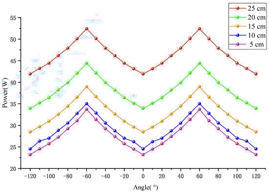
Figure 4.
Modeling and validation of the effect on the power consumption by the center of gravity position.
Concerning the distance axis, the power consumption of the robot does not increase symmetrically with distance but in an exponential manner. This is because the farther the robot’s center of gravity is from the geometric center, the more entire mass is pressed against one of the robot’s driving motors, which leads to a sharp increase in the power consumption of the robot’s motors at the corresponding location, and the power consumption of the robot increases exponentially. So we generally recommend a strategy of placing objects in the middle as much as possible.
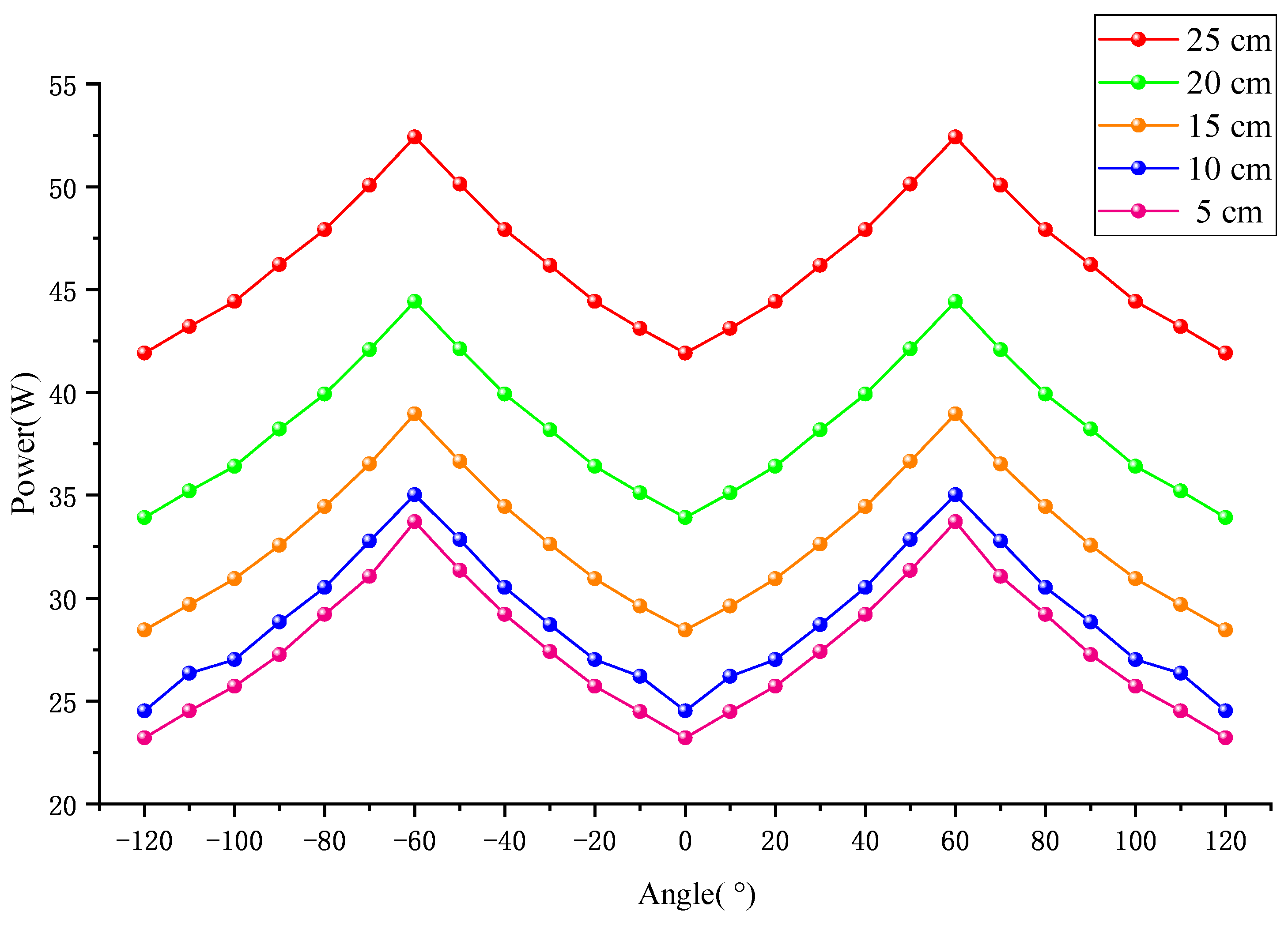
Figure 5 shows the comparison between the modeled data and measured data of power consumption when the robot is moving at different angles. In order to verify the symmetry of the energy consumption, we selected the region centered on the positive direction of the Y-axis of the robot coordinate system, 60 degrees to the left and right. To fully showcase the symmetrical characteristics of power consumption, we avoided adding additional counterweights during the experiment. This approach ensures that the center of gravity and the geometric center of the robot remain aligned. It can be observed that the pattern of the power consumption is fully consistent with our model, and the power consumption is symmetrically distributed according to 60 degrees. Due to the special structure of the TOMR, the three drive wheels are completely symmetrical, so the power consumption shows the symmetrical distribution of 120 degrees. Additionally, when the robot moves in two opposite directions, the power consumption is identical. Therefore, the overall power consumption demonstrates a symmetrical distribution at 60-degree intervals.
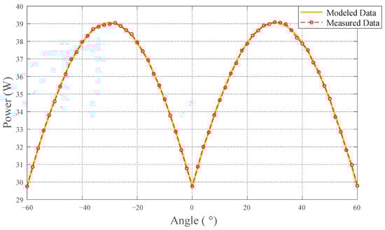
Figure 5.
The influence of the robot’s motion direction on power consumption.
3. Analysis of Typical Robot Faults
In a review paper, Muhamad et al. [43] analyzed hardware and software faults in robotic systems and concluded that hardware faults are the most common and require real-time identification and correction. Demetris et al. [44] employed a model-based on a Luenberger observer for actuator fault detection in differential-drive mobile robots, validating that their method effectively detects and identifies various faults. Therefore, according to their study and the previous literature, the main possible faults in the robot are control system faults, motor encoder faults, motor faults, and robot slippage. In the following, we analyze the energy consumption characteristics of these faults individually.
To fully illustrate the power consumption characteristics associated with faults and to enable as accurate a diagnosis of the machine’s faults as possible, we set the robot to move in three specific directions: 20 degrees from the negative direction of the Y-axis in the robot’s coordinate system, a direction parallel to the second drive wheel, and a direction parallel to the first drive wheel. These four directions are selected mainly because the robot motion along these four directions can well reflect the motion characteristics of the omnidirectional-wheel robot, and at the same time, the robot has different characteristics of power consumption when it performs the motion in these four directions, which can provide sufficient data for the robot fault diagnosis. The power consumption curve of the robot in the absence of faults is shown in Figure 6.
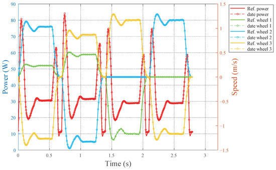
Figure 6.
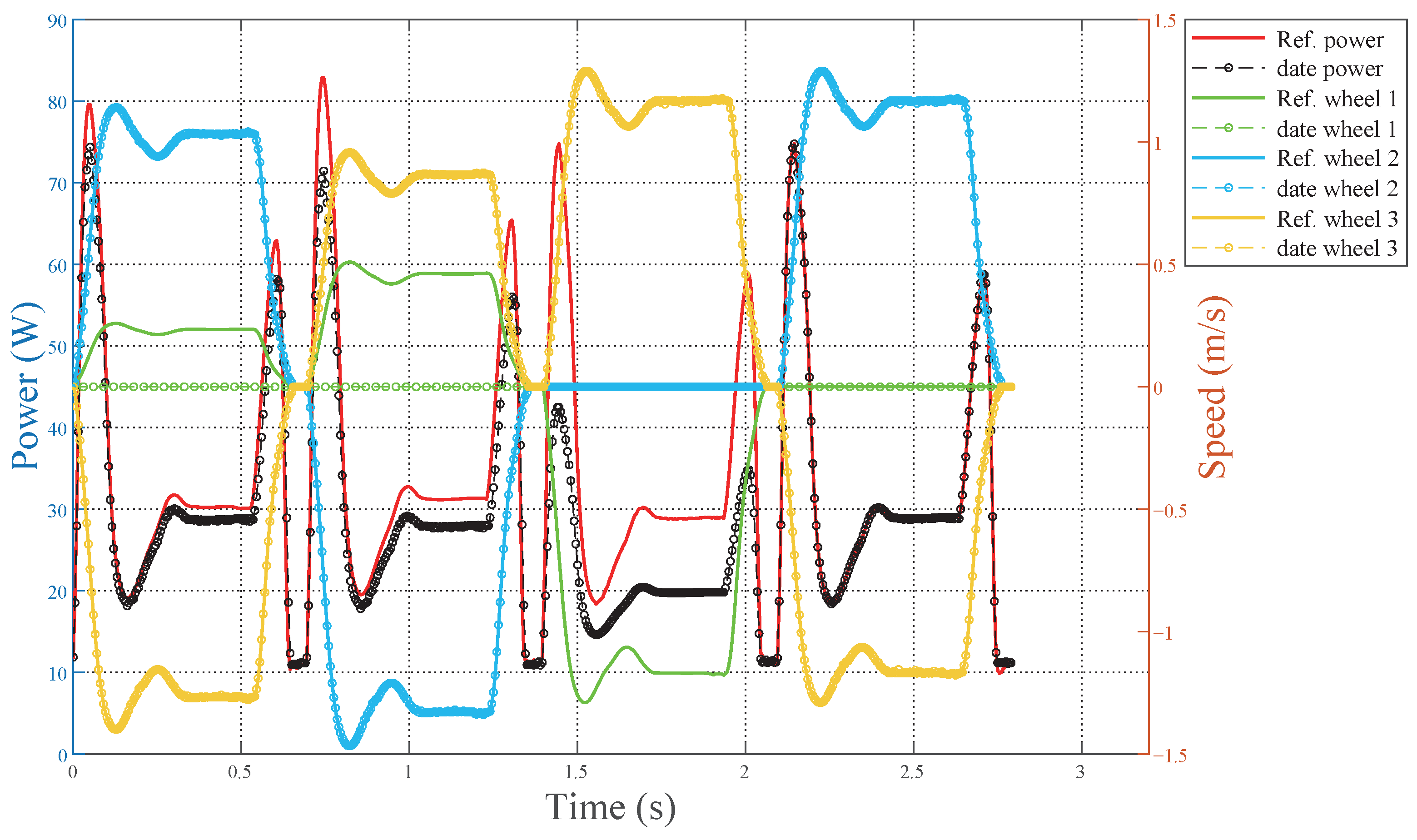
The modeled and measured data in healthy robot condition.
When the robot is healthy, the modeled values for the power consumption and speed match very well with the measured values during the actual operation. Only in the two phases of acceleration and braking, where the speed and power consumption change drastically, the modeled value has a minor error from the actual measured value. After measurement, the discrepancies between the modeled and observed data for power consumption and speed are minimal, fully satisfying the requirements for fault diagnosis.
3.1. Fault in the Control System
The first issue involves a fault in the control system. To address this, we employ a method where the control signal to motor no. 1 is disconnected, effectively removing any control signal input to its drive. This simulates a scenario where the robot’s control system experiences a sudden fault during operation, resulting in no control signal output. The motion process for the experiment is conducted in four stages, as previously described, and the characteristic curve of the power consumption is illustrated in Figure 7.
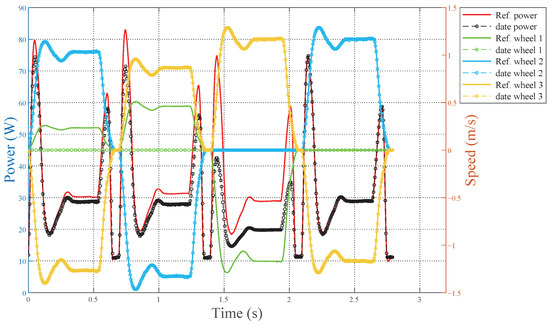
Figure 7.
The modeledand measured data in the case of control system faults.
It is evident that the speed of motor no. 1 is always 0 because of the fault of the control system. It is also apparent that the actual measured power consumption of the robot is always less than or equal to the theoretical modeled value because of the absence of the control signal of motor no. 1. Motor no. 1 has no drive signal, so there is only standby power consumption and no motion power consumption . During the stationary phase, as well as during the fourth motion, the measured values of the robot power consumption and the theoretical modeled values are the same because motor no. 1 does not need to move. During other movements, the error between the measured and theoretical modeled values of the power consumption increases as the speed of motor no. 1 increases. Through the above process, it can be found that simply looking at one process it is impossible to accurately learn whether the robot is faulty or not, which is why we use four directions of the movement.
3.2. Fault of Encoder
Another possible fault of the robot is a fault in the motor encoder, because the motor and encoder are often inlaid together; so, in this fault diagnosis we combine the encoder fault and the motor fault into one category, collectively called the motor system fault. When setting the encoder fault, we cut the encoder data line of motor no. 1, so the encoder data of motor no. 1 will not be input to the control system, and the error between the measured power consumption of the robot and the modeled theoretical value is shown in Figure 8.
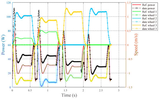
Figure 8.
The modeled and measured data in the case of encoder faults.
It can be observed that when the robot needs motor no. 1 to move, the encoder data of motor no. 1 cannot be uploaded to the control system due to the encoder fault, and the control system judges that motor no. 1 is always in the static state according to the encoder data. Due to the control of PID regulation, the control system will keep sending acceleration signals to the controller of motor no. 1, so motor no. 1 will always be in the acceleration state until the speed reaches the maximum. Afterward, motor no. 1 will continue operating at full speed until the braking stage. In the braking phase, the control system will judge the speed of each driving wheel, and then, send the braking signal to the controller of each motor, which is to send the signal of reverse acceleration to the motor controller. However, since the encoder of motor no. 1 is not sending data to the control system at this time, the control system always thinks that motor no. 1 is at a standstill and does not need braking, and the control system will stop sending control signals. At this time, motor no. 1 is in the state of loss of control, because motor no. 1 does not have the braking process. Instead, during the final stop, part of the kinetic energy of the robot is converted into electrical energy, so the measured value of the power consumption during the braking process is less than the theoretical value of the power consumption modeling.
However, in the braking phase, if we only look at the measured values and the modeled value of the robot’s energy consumption, as well as the measured values and the modeled value of the speed, it is the same phenomenon as the loss of the control signal. Therefore, we add a pair of comparison quantities: the actual measured value of the robot’s power consumption and the power consumption value solved from the encoder data. When the robot loses the control signal, the measured values of the power consumption and the power consumption solved by the encoder data are the standby power consumption values ; the power consumption values solved from the encoder data when the robot loses the signal from the encoder are shown in Figure 9.
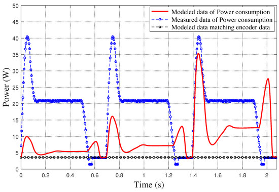
Figure 9.
Comparison between modeled data of power consumption, measured data of power consumption, and power consumption solved from encoder data.
It can be seen that with the loss of the encoder signal, the power consumption solved from the encoder data is always the standby power consumption of the motor . In most cases, the actual measured power consumption is significantly higher than the power consumption calculated from the encoder data and the theoretical modeled power consumption value.
3.3. Robot Slips
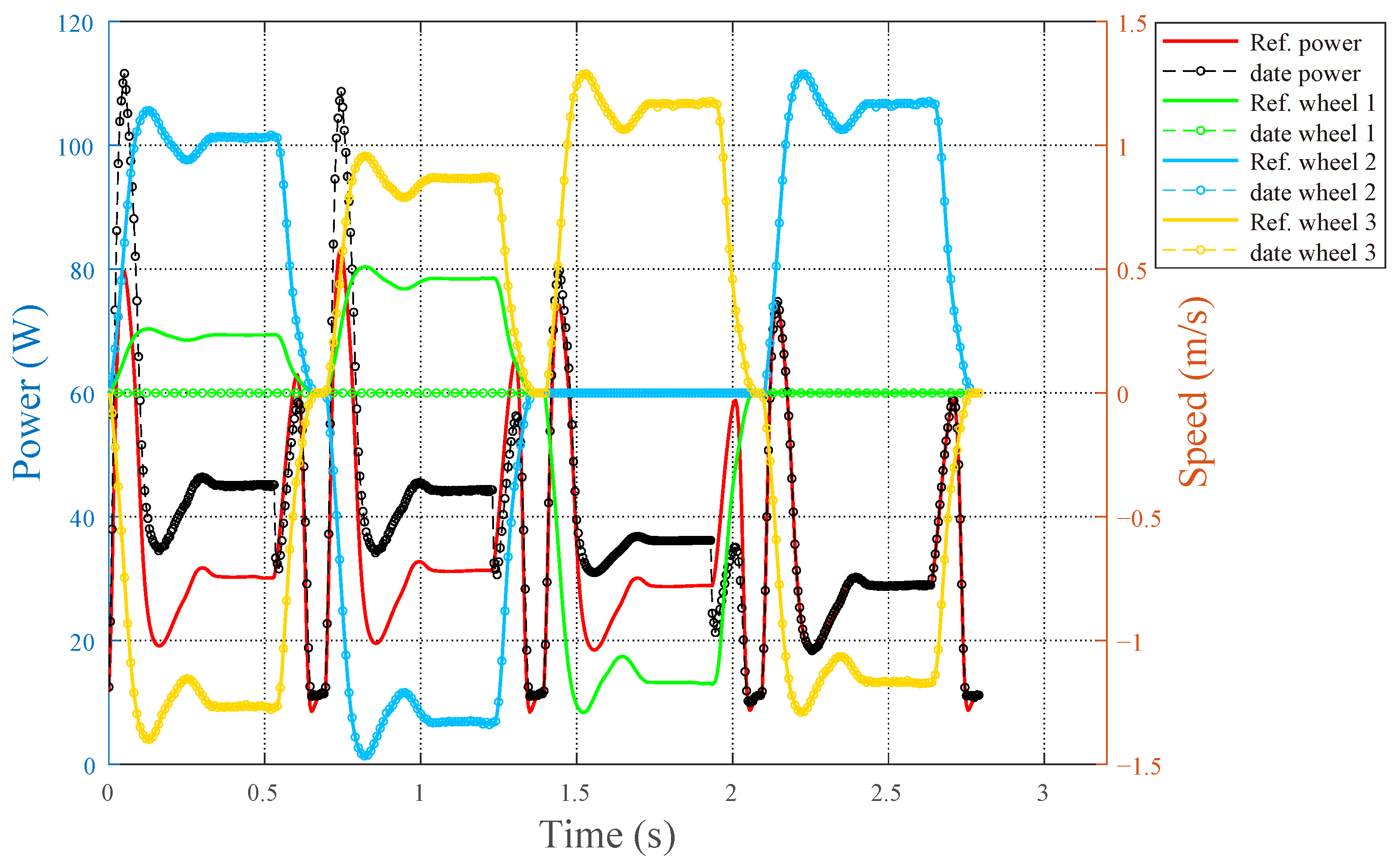
If the static friction between the omnidirectional wheel and the ground is too small to transmit the torque output by the motor fully, the slip fault will occur. For the experimental scenario setup of slipping, the method we used was to place the robot on smooth ground and add lubricators on it to reduce the static friction between the drive wheels and the ground, and ensure that the robot would slip when running on it. The robot will slip strongly when it moves on this kind of surface. A comparison between the measured and modeled theoretical values of the robot power consumption in the case of slip is shown in Figure 10.
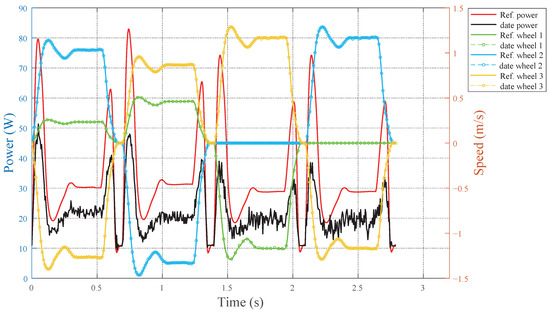
Figure 10.
The modeled and measured data in the case of slip.
The power consumption of the robot is drastically changed in the case of slip, because the slip state is one of the runaway states of the robot. At this point, the robot has lost the ability to adjust the speed, and can only control the motor to rotate according to the pre-set speed. Still, the output of the motor is not fully converted into kinetic energy of the robot, and most of it is lost with the slippage between the omnidirectional wheel and the surface.
During the robot slippage, the control system is completely unable to control the robot’s movement, and this is very dangerous for robots. However, problems such as control system faults may also cause similar phenomena to robot slippage, so the robot needs to determine the cause and take different actions.
4. Fault Diagnosis Based on ANN
If using models for fault diagnosis, it is necessary to construct separate energy consumption models for each fault. Subsequently, robot faults are determined based on these tailored fault–energy consumption models. However, because the severity of faults varies, distinguishing them using this method requires numerous power consumption models, which may not be practical. In essence, robot fault diagnosis is a classification problem, and an effective method to address this classification challenge is through the use of artificial neural networks (ANNs). For example, Shifat et al. [45] utilized an ANN for fault diagnosis in brushless DC motors (BLDCs) using multi-sensor data, achieving high-precision fault detection and classification.
Here, we use the most straightforward ANN, an ANN with a single hidden layer, to solve the fault diagnosis problem. As shown in Figure 11, the ANN network structure consists of an input layer with 10 neurons, a single hidden layer, and an output layer with six outputs representing six different types of states. The 10 inputs for the neurons are:
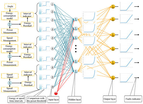
Figure 11.
Fault diagnosis by ANN.
- (1)
- Four inputs representing the residuals between the modeled and actual measured energy consumption values compared to the threshold values, with three of these inputs for each motor and one for the total energy consumption.
- (2)
- Three inputs representing the residuals between the energy consumption values derived from the encoder data and the actual measured values compared to the threshold values, with each input corresponding to one motor.
- (3)
- Three inputs representing the residuals between the modeled and actual measured motor speed values compared to the threshold values, with each input corresponding to one motor.
Due to the inevitable discrepancies between the modeled values and the actual measured values of speed and power consumption, we set thresholds for the residuals when inputting them into the ANN, as shown in the following Equations (18)–(20):
where r is the energy residual, calculated as the difference between the measured and modeled values of power consumption. The threshold range for the energy residuals is set at , meaning the measured value of energy consumption can deviate from the modeled value by more than 5% or less than 5%. This range is considered normal if the residual distribution falls within it. Our tests indicate that residuals within this range do not affect the robot’s normal operation.
The same operation is used for the speed, except that we set the speed threshold differently. This is because fluctuations in speed are generally less significant compared to power consumption, which can vary slightly due to factors like the loosening of the robot’s structure, its motor, or the drive wheels. Unlike these factors, speed fluctuations are typically not as affected by such issues.
For the inputs of the ANN network’s input layer, we simplify the inputs to ‘0’, ‘1’, or ‘−1’, as shown in Equation (21). When the energy residuals are within the threshold range of −5% to +5%, they are represented by ‘0’. When the energy residuals exceed the +5% threshold, they are represented by ‘1’. When the energy residuals fall below the −5% threshold, they are represented by ‘−1’.
Based on the experiments, the optimal results were achieved when the input layer of the ANN had 10 neurons and the single hidden layer was set to 30 neurons. Additionally, the output layer consisted of 6 neurons, representing six different states of the robot: normal (), slipping (), control system fault (), motor system fault in no. 1 (), motor system fault in no. 2 (), and motor system fault in no. 3 (). The hyperparameters were set as follows: a learning rate of 0.01, ReLU activation for the hidden layer, Softmax activation for the output layer, Adam optimizer, categorical cross-entropy loss, a batch size of 32, and 100 training epochs.
Table 1 and Table 2 show the input and output of the fault diagnosis neural network, respectively, and each column of Table 1 shows the input data of the neural network. The final target output of each column is the output expected by the neural network. Each row of Table 2 shows the output of the neural network, and the criterion for fault indication is the maximum value in each output vector. By comparing the data in Table 1 and the results in Table 2, we can conclude that the accuracy of the test model is as high as 98%.

Table 1.
The ANN’s input and target output.
Table 2.
Fault diagnosis ANN output results.
5. Conclusions
In this paper, we propose a data-driven fault diagnosis technique to determine the current state of the robot by monitoring its power consumption during operation. Initially, we construct the energy model of a TOMR, into which the basic state of the robot is input to obtain reference data from the model. These modeled data are then compared with the actual measured data to calculate the data residuals. Based on the distribution of these residuals, an ANN is employed to identify issues such as robot slippage or other faults. While the method can be extended to other wheeled robots, it is specifically tailored to TOMRs. Adapting it to different robot types may require significant adjustments. The main conclusions of this study can be summarized as follows:
- (1)
- The energy model of the TOMR was constructed, and its accuracy was significantly enhanced by incorporating factors affecting power consumption as parameters within the model. The accuracy of this energy model was measured to be approximately 97%.
- (2)
- The proposed method can quickly and accurately identify various faults in the robot and pinpoint the causes of robot slippage. However, this approach requires encoder data and real-time measured data of power consumption.
- (3)
- By feeding energy residuals and velocity residuals into a simple ANN, the type of fault occurring in the robot can be determined very accurately without the need for complex timing information and a long network training process.
- (4)
- The proposed energy model and fault diagnosis method can be extended to other wheeled robots by very simple transformations.
In the future, given that we can already identify the type of robot slippage that occurs, our next steps will involve adopting different strategies for various faults. Additionally, we aim to determine the degree of slippage and perform odometer correction based on the energy consumption model when slippage occurs.
Author Contributions
Conceptualization, B.W. and L.Z.; methodology, B.W.; software, B.W.; validation, B.W., L.Z. and J.K.; formal analysis, J.K.; investigation, L.Z.; resources, L.Z.; data curation, B.W.; writing—original draft preparation, B.W.; writing—review and editing, B.W.; visualization, J.K.; supervision, L.Z.; project administration, L.Z.; funding acquisition, L.Z. All authors have read and agreed to the published version of the manuscript.
Funding
This project was supported by the Natural Science Foundation of Shandong Province, China (No. ZR2020MF073).
Data Availability Statement
The data presented in this study are available on request from the corresponding author.The data are not publicly available due to restrictions imposed by the data provider.
Conflicts of Interest
The authors declare no conflicts of interest.
Abbreviations
The following abbreviations are used in this manuscript:
| ANN | Artificial neural network |
| EBM | Energy-based maintenance |
| EKF | Extended Kalman filter |
| IMU | Inertial measurement unit |
| PTESO | Prescribed-time extended state observer |
| PID | Proportional–integral–derivative |
| TOMR | Three-wheeled omnidirectional mobile robot |
| VO | Visual odometry |
References
- Kim, H.; Kim, B. Minimum-energy cornering trajectory planning with self-rotation for three-wheeled omni-directional mobile robots. Int. J. Control. Autom. Syst. 2017, 15, 1857–1866. [Google Scholar] [CrossRef]
- Li, Y.; Dai, S.; Zhao, L.; Yan, X.; Shi, Y. Topological design methods for mecanum wheel configurations of an omnidirectional mobile robot. Symmetry 2019, 11, 1268. [Google Scholar] [CrossRef]
- Kassawat, M.; Cervera, E.; del Pobil, A. An omnidirectional platform for education and research in cooperative robotics. Electronics 2022, 11, 499. [Google Scholar] [CrossRef]
- Wang, D.; Yi, J.; Zhao, D.; Yang, G. Teleoperation system of the internet-based omnidirectional mobile robot with a mounted manipulator. In Proceedings of the International Conference on Mechatronics and Automation, Harbin, China, 5–8 August 2007; pp. 1799–1804. [Google Scholar] [CrossRef]
- Kebritchi, A.; Hosseiniakram, P.; Havashinezhadian, S.; Rostami, M. Design and development of an omnidirectional mobile manipulator for indoor environment. In Proceedings of the International Conference on Robotics and Mechatronics, Tehran, Iran, 23–25 October 2018; pp. 152–158. [Google Scholar] [CrossRef]
- Vandewal, B.; Gillis, J.; Pipeleers, G.; Swevers, J. Simplified wheel slip modeling and estimation for omnidirectional vehicles. In Proceedings of the IEEE 17th International Conference on Advanced Motion Control (AMC), Padova, Italy, 18–20 February 2022; pp. 389–395. [Google Scholar] [CrossRef]
- Han, K.L.; Kim, H.; Lee, J.S. The sources of position errors of omnidirectional mobile robots with Mecanum wheels. In Proceedings of the IEEE International Conference on Systems, Man and Cybernetics, Istanbul, Turkey, 10–13 October 2010; pp. 581–586. [Google Scholar] [CrossRef]
- Ward, C.C.; Iagnemma, K. A dynamic-model-based wheel slip detector for mobile robots on outdoor terrain. IEEE Trans. Robot. 2008, 24, 821–831. [Google Scholar] [CrossRef]
- Zhang, S.; Chen, Y.; tao Chen, S.; Zheng, N. Hybrid A*-based curvature continuous path planning in complex dynamic environments. In Proceedings of the IEEE Intelligent Transportation Systems Conference (ITSC), Auckland, New Zealand, 27–30 October 2019; pp. 1468–1474. [Google Scholar] [CrossRef]
- Song, X.; Shao, Y.; Qu, Z. A vehicle trajectory tracking method with a time-varying model based on the model predictive control. IEEE Access 2020, 8, 16573–16583. [Google Scholar] [CrossRef]
- Liao, Y.; Hashemi, E.; Wang, T.; Yang, B. A learning-aided generic framework for fault detection and recovery of inertial sensors in automated driving systems. IEEE Syst. J. 2020, 15, 3001–3011. [Google Scholar] [CrossRef]
- Sekaran, J.F.; Kaluvan, H.; Irudhayaraj, L. Modeling and analysis of GPS-GLONASS navigation for car-like mobile robots. J. Electr. Eng. Technol. 2020, 15, 927–935. [Google Scholar] [CrossRef]
- Bao, J.; Yao, X.; Tang, H.; Song, A. Outdoor navigation of a mobile robot by following GPS waypoints and local pedestrian lane. In Proceedings of the IEEE 8th Annual International Conference on CYBER Technology in Automation, Control, and Intelligent Systems (CYBER), Tianjin, China, 19–23 July 2018; IEEE: Piscataway, NJ, USA, 2018; pp. 198–203. [Google Scholar] [CrossRef]
- Gharajeh, M.S.; Jond, H.B. Hybrid global positioning system-adaptive neuro-fuzzy inference system based autonomous mobile robot navigation. Robot. Auton. Syst. 2020, 134, 103669. [Google Scholar] [CrossRef]
- Wang, Y.; Liu, X.; Kang, Y.; Ge, S.S. Anomaly-resilient relative pose estimation for multiple nonholonomic mobile robot systems. IEEE Syst. J. 2020, 16, 659–670. [Google Scholar] [CrossRef]
- Chang, P.; Fan-Chiang, S.; Chen, C.; Lan, C. Real-time fault detection for Mecanum wheel omnidirectional robot platform. In Proceedings of the 21st International Conference on Control, Automation and Systems (ICCAS), Jeju, Korea, 12–15 October 2021; IEEE: Piscataway, NJ, USA, 2021; pp. 1969–1973. [Google Scholar] [CrossRef]
- Gustafsson, F. Slip-based tire-road friction estimation. Automatica 1997, 33, 1087–1099. [Google Scholar] [CrossRef]
- Ojeda, L.; Reina, G.; Borenstein, J. Experimental results from FLEXnav: An expert rule-based dead-reckoning system for Mars rovers. In Proceedings of the IEEE Aerospace Conference Proceedings (IEEE Cat. No. 04TH8720), Big Sky, MT, USA, 6–13 March 2004; IEEE: Piscataway, NJ, USA, 2004; Volume 2, pp. 816–825. [Google Scholar] [CrossRef]
- Krishnamoorthy, G.; Ashok, P.; Tesar, D. Simultaneous sensor and process fault detection and isolation in multiple-input–multiple-output systems. IEEE Syst. J. 2015, 9, 335–349. [Google Scholar] [CrossRef]
- Ojeda, L.; Cruz, D.; Reina, G.; Borenstein, J. Current-based slippage detection and odometry correction for mobile robots and planetary rovers. IEEE Trans. Robot. 2006, 22, 366–378. [Google Scholar] [CrossRef]
- Malinowski, M.T.; Richards, A.; Woods, M. Fusion of visual and wheel odometry with integrated slip estimation. In Proceedings of the AIAA Scitech 2021 Forum, Virtual Event, 19–21 January 2021; p. 1757. [Google Scholar] [CrossRef]
- Liu, Y.; Zhao, C.; Ren, M. An enhanced hybrid visual-inertial odometry system for indoor mobile robots. Sensors 2022, 22, 2930. [Google Scholar] [CrossRef] [PubMed]
- Birem, M.; Kleihorst, R.; El-Ghouti, N. Visual odometry based on the Fourier transform using a monocular ground-facing camera. J. -Real-Time Image Process. 2018, 14, 637–646. [Google Scholar] [CrossRef]
- Angelova, A.; Matthies, L.; Helmick, D.; Sibley, G.; Perona, P. Learning to predict slip for ground robots. In Proceedings of the Proceedings 2006 IEEE International Conference on Robotics and Automation, ICRA 2006, Orlando, FL, USA, 15–19 May 2006; IEEE: Piscataway, NJ, USA, 2006; pp. 3324–3331. [Google Scholar] [CrossRef]
- Sidek, N.; Sarkar, N. Integrating actuator fault and wheel slippage detections within FDI framework. WSEAS Trans. Syst. 2007, 6, 298. [Google Scholar]
- Sabry, A.H.; Nordin, F.H.; Sabry, A.H.; Ab Kadir, M.Z.A. Fault detection and diagnosis of industrial robot based on power consumption modeling. IEEE Trans. Ind. Electron. 2019, 67, 7929–7940. [Google Scholar] [CrossRef]
- Orošnjak, M.; Brkljač, N.; Šević, D.; Čavić, M.; Oros, D.; Penčić, M. From predictive to energy-based maintenance paradigm: Achieving cleaner production through functional-productiveness. J. Clean. Prod. 2023, 408, 137177. [Google Scholar] [CrossRef]
- Morales, J.; Martinez, J.L.; Mandow, A.; Garcia-Cerezo, A.J.; Pedraza, S. Power consumption modeling of skid-steer tracked mobile robots on rigid terrain. IEEE Trans. Robot. 2009, 25, 1098–1108. [Google Scholar] [CrossRef]
- Wang, Y.; Xiong, W.; Yang, J.; Jiang, Y.; Wang, S. A robust feedback path tracking control algorithm for an indoor carrier robot considering energy optimization. Energies 2019, 12, 2010. [Google Scholar] [CrossRef]
- Liu, S.; Sun, D. Minimizing energy consumption of wheeled mobile robots via optimal motion planning. IEEE/ASME Trans. Mechatronics 2013, 19, 401–411. [Google Scholar] [CrossRef]
- Xu, W.; Liu, H.; Liu, J.; Zhou, Z.; Pham, D.T. A practical energy modeling method for industrial robots in manufacturing. In Challenges and Opportunity with Big Data: 19th Monterey Workshop 2016, Beijing, China, 8–11 October 2016; Springer: Berlin/Heidelberg, Germany, 2016; pp. 25–36. [Google Scholar] [CrossRef]
- Burghi, T.B.; Iossaqui, J.G.; Camino, J.F. Kinematic control design for wheeled mobile robots with longitudinal and lateral slip. arXiv 2021. [Google Scholar] [CrossRef]
- Song, J.; Kumar, P.; Kim, Y.; Kim, H. A Fault Detection System for Wiring Harness Manufacturing Using Artificial Intelligence. Mathematics 2024, 12, 537. [Google Scholar] [CrossRef]
- Hendzel, Z.; Trojnacki, M. Adaptive fuzzy control of a four-wheeled mobile robot subject to wheel slip. Wseas Trans. Syst. 2023, 22, 602–612. [Google Scholar] [CrossRef]
- Li, Z.; Zhao, Y.; Yan, H.; Wang, M.; Zeng, L. Prescribed-time zero-error active disturbance rejection control for uncertain wheeled mobile robots subject to skidding and slipping. Int. J. Syst. Sci. 2023, 54, 1313–1329. [Google Scholar] [CrossRef]
- Jaramillo-Morales, M.F.; Dogru, S.; Marques, L.; Gomez-Mendoza, J.B. Predictive power estimation for a differential drive mobile robot based on motor and robot dynamic models. In Proceedings of the IEEE International Conference on Robotic Computing (IRC), Naples, Italy, 25–27 February 2019; IEEE: Piscataway, NJ, USA, 2019; pp. 301–307. [Google Scholar] [CrossRef]
- Jaramillo-Morales, M.F.; Dogru, S.; Gomez-Mendoza, J.B.; Marques, L. Energy estimation for differential drive mobile robots on straight and rotational trajectories. Int. J. Adv. Robot. Syst. 2020, 17, 1729881420909654. [Google Scholar] [CrossRef]
- Wang, J.; Chen, J.; Xiao, Q. A minimum-energy trajectory tracking controller for four-wheeled omni-directional mobile robots. In Proceedings of the 15th International Conference on Control, Automation, Robotics and Vision (ICARCV), Singapore, 18–21 November 2018; IEEE: Piscataway, NJ, USA, 2018; pp. 48–53. [Google Scholar] [CrossRef]
- Xie, L.; Henkel, C.; Stol, K.; Xu, W. Power-minimization and energy-reduction autonomous navigation of an omnidirectional Mecanum robot via the dynamic window approach local trajectory planning. Int. J. Adv. Robot. Syst. 2018, 15, 1729881418754563. [Google Scholar] [CrossRef]
- Xie, L.; Herberger, W.; Xu, W.; Stol, K.A. Experimental validation of energy consumption model for the four-wheeled omnidirectional mecanum robots for energy-optimal motion control. In Proceedings of the IEEE 14th International Workshop on Advanced Motion Control (AMC), Auckland, New Zealand, 22–24 April 2016; IEEE: Piscataway, NJ, USA, 2016; pp. 565–572. [Google Scholar] [CrossRef]
- Hou, L.; Zhang, L.; Kim, J. Energy modeling and power measurement for three-wheeled omnidirectional mobile robots for path planning. Electronics 2019, 8, 843. [Google Scholar] [CrossRef]
- Kim, H.; Kim, B.K. Online minimum-energy trajectory planning and control on a straight-line path for three-wheeled omnidirectional mobile robots. IEEE Trans. Ind. Electron. 2014, 61, 4771–4779. [Google Scholar] [CrossRef]
- Alobaidy, M.A.; Abdul-Jabbar, J.; Al-khayyt, S. Faults diagnosis in robot systems: A review. Al-Rafidain Eng. J. 2020, 25, 166–177. [Google Scholar] [CrossRef]
- Stavrou, D.; Eliades, D.G.; Panayiotou, C.; Polycarpou, M. Fault detection for service mobile robots using model-based method. Auton. Robot. 2015, 40, 383–394. [Google Scholar] [CrossRef]
- Shifat, T.A.; Hur, J.W. ANN Assisted Multi Sensor Information Fusion for BLDC Motor Fault Diagnosis. IEEE Access 2021, 9, 9429–9441. [Google Scholar] [CrossRef]


Disclaimer/Publisher’s Note: The statements, opinions and data contained in all publications are solely those of the individual author(s) and contributor(s) and not of MDPI and/or the editor(s). MDPI and/or the editor(s) disclaim responsibility for any injury to people or property resulting from any ideas, methods, instructions or products referred to in the content. |
© 2024 by the authors. Licensee MDPI, Basel, Switzerland. This article is an open access article distributed under the terms and conditions of the Creative Commons Attribution (CC BY) license (https://creativecommons.org/licenses/by/4.0/).