Bias-Correction Methods for the Unit Exponential Distribution and Applications

Abstract

The bias of the maximum likelihood estimator can cause a considerable estimation error if the sample size is small. To reduce the bias of the maximum likelihood estimator under the small sample situation, the maximum likelihood and parametric bootstrap bias-correction methods are proposed in this study to obtain more reliable maximum likelihood estimators of the unit exponential distribution parameters. The procedure to implement the bias-corrected maximum likelihood estimation method is derived analytically, and the steps to obtain the bias-corrected bootstrap estimators are presented. The simulation results show that the proposed maximum likelihood bootstrap bias-correction method can significantly reduce the bias and mean squared error of the maximum likelihood estimators for most of the parameter combinations in the simulation study. A soil moisture data set and a numerical example are used for illustration.

1. Introduction

In some instances, we must use proportional variables for modeling. In common cases, for example, we need to make inferences about the proportions of successes; party votes; the consumption of a cause; and specific public event attendance. The applications can be found in social studies, economics, healthcare, engineering, and more.

1.1. Literature Review

The popular modeling process of a proportional sample involves considering a random variable over a range between 0 and 1. Thus, the Beta distribution proposed by Bayes [1] has been widely used to make inferences in the applications of proportional sample modelings, for example, by Fleiss et al. [2], Gilchrist [3], and Seber [4]. However, the Beta distribution is not suitable for all applications. Besides Beta one, many other distributions have been suggested in the literature. Leipnik [5] proposed an approximate distribution of the serial correlation coefficient as a circular universe. Johnson [6] suggested the unit Johnson distribution. Topp and Leone [7] studied a family of the J-shaped cumulative frequency function. Consul and Jain [8] proposed the unit gamma distribution. Kumaraswamy [9] considered a generalized distribution for double-bounded variables. Jørgensen [10] studied a subclass of dispersion models, which are the proper four-parameter dispersion models.

In recent decades, many works have studied the unit interval distribution functions. Smithson and Shou [11] worked on the cumulative distribution function (CDF) and quantile distribution over the unit interval. Altun and Hamedani [12] studied the log-xgamma distribution. Nakamura et al. [13] proposed a new unit interval distribution. Ghitany et al. [14] suggested the unit-inverse Gaussian distribution. Moreover, the unit Gompertz, unit Lindley, and unit Weibull distributions have been studied by Mazucheli et al. [15,16,17]. Altun [18] probed the log-weighted exponential distribution. Gündüz et al. [19] investigated the unit Johnson $S_U$ distribution. Biswas and Chakraborty [20] constructed absolutely continuous distributions over the unit interval. They used two absolutely continuous random variables with non-negative support to generate the conditional distribution for one of them, given their sum as one through the convolution concept. Afify et al. [21] proposed another new unit distribution. Krishna et al. [22] studied the unit Teissier distribution. Korkmaz and Korkmaz [23] worked on the unit log–log distribution. Fayomi et al. [24] suggested the unit–power Burr X distribution. Bakouch et al. [25] proposed a new unit exponential distribution and concluded that the aforementioned approaches are mainly based on conventional strategies, including (1) log transformation approaches, (2) the CDF and quantile methodology, (3) reciprocal transformation, (4) exponential transformation, (5) the conditional distribution methodology, and (6) the T-X family approach. Bakouch et al. [25] used the epsilon function,

$$\begin{array}{c}\hfill {ϵ}_{\lambda ,a}={\left(\frac{a+x}{a-x}\right)}^{\frac{\lambda a}{2}},x\in (-a,a);\mathrm{otherwise},{ϵ}_{\lambda ,a}=0,\end{array}$$

(1)

where $\lambda \in {\mathbb{R}}^{+}$ and $a>0$. Dombi et al. [26] provided a detailed procedure for establishing the unit exponential distribution.

The unit exponential distribution proposed by Bakouch et al. [25] is more flexible for modeling than the aforementioned ones and can exhibit either negative or positive skewness. They also showed that the proposed unit exponential distribution has an increasing failure rate or belongs to the decreasing mean residual life class if $\lambda >0$. They also proposed the maximum likelihood estimation process to obtain the estimators of model parameters.

1.2. The Motivation and Organization

In some situations, we could use the unit exponential distribution proposed by Bakouch et al. [25] with a small-sized sample for statistical inference. It is important to know how to reduce the estimation bias with a small-sized sample. In this study, we propose an analytic bias-corrected maximum likelihood estimation method to reduce the estimation bias. Then, random samples will be generated from the unit exponential distribution to verify the performance of the proposed bias-corrected maximum likelihood estimation method. Moreover, a bias-corrected parametric bootstrap estimation procedure is also proposed to compete with the proposed bias-corrected maximum likelihood estimation method. The second bias-correction procedure relies on heavy computer computation but not on the deviation process of mathematical approximation. This study aims to provide feasible and simple methods to reduce the bias and mean square error of the maximum likelihood estimators of the unit exponential distribution when the sample size is small. The proposed method will be illustrated with one numerical example and one soil moisture example to demonstrate the applications.

In summary, three contributions are included in this study to reduce the bias of the maximum likelihood estimator of the unit exponential distribution parameters:

• An analytical procedure of the maximum likelihood bias-correction method is proposed.
• The implementation of the parametric bootstrap bias-correction method is proposed.
• The performance of the two proposed bias-correction methods is studied using Monte Carlo simulations. We find that the proposed maximum likelihood bias-correction method is more competitive than the other two competitors.

There are five sections in this article. The unit exponential distribution and maximum likelihood estimation procedure will be briefly reviewed in Section 2. Section 3 addresses the detailed derivation of the proposed bias-corrected maximum likelihood estimation method and bias-corrected parametric bootstrap procedure. In Section 4, Monte Carlo simulations are conducted to evaluate the performance of both bias-corrected estimation methods. One example is presented in Section 5 to demonstrate the application of both estimation methods. Some concluding remarks are made in Section 6.

2. The Unit Exponential Distribution and Maximum Likelihood Estimation

Let X be a bounded random variable having support over 0 to 1 and ${\Theta }^T=({\theta }_1,{\theta }_2)=(\alpha ,\beta )$. The cumulative density function (CDF) of the unit exponential distribution can be defined by

$$\begin{array}{c}\hfill F\left(x\right|\Theta )=1-exp\left\{\alpha \left(1-{\left(\frac{1+x}{1-x}\right)}^{\beta }\right)\right\},\end{array}$$

(2)

if $0\le x<1$, and 1, if $x=1$, where $\alpha$ and $\beta$ are positive unknown parameters. Denote the distribution of (2) by $X\sim \mathrm{UED}(\alpha ,\beta )$. $F\left(x\right|\alpha ,\beta )$ in (2) can be represented by

$$\begin{array}{c}\hfill F\left(x\right|\Theta )=1-exp\left\{\alpha \left(1-{ϵ}_{2\beta ,1}\left(x\right)\right)\right\}.\end{array}$$

(3)

Let $f\left(x\right|\Theta )=\frac{dF\left(x\right|\Theta )}{dx}$; the probability density function (PDF) of $\mathrm{UED}(\alpha ,\beta )$ can be obtained by

$$\begin{array}{c}\hfill f\left(x\right|\Theta )=\frac{2\alpha \beta }{1-x^2}{\left(\frac{1+x}{1-x}\right)}^{\beta }exp\left\{\alpha \left(1-{\left(\frac{1+x}{1-x}\right)}^{\beta }\right)\right\},0<x<1.\end{array}$$

(4)

Let $x_p$ be the pth quantile of $\mathrm{UED}(\alpha ,\beta )$, $0<p<1$. Utilizing the CDF of Equation (2), one can set $p=F\left(x_p\right|\Theta )$. Then, $x_p$ can be presented by

$$\begin{array}{c}\hfill x_p=\frac{{\left(1-\frac{1}{\alpha }log(1-p)\right)}^{\frac{1}{\beta }}-1}{{\left(1-\frac{1}{\alpha }log(1-p)\right)}^{\frac{1}{\beta }}+1},0<p<1,\end{array}$$

(5)

because the support of X is a subset of positive reals. Using the formula $m_r=E\left(x^r\right)=r{\int }_0^1{x}^{r-1}\{1-F\left(x\right)\}dx$, the rth moment of $\mathrm{UED}(\alpha ,\beta )$ can be presented by

$$\begin{array}{c}\hfill m_r=r{e}^{\alpha }{\int }_0^1{x}^{r-1}exp\left\{-\alpha {\left(\frac{1+x}{1-x}\right)}^{\beta }\right\}dx,r=1,2,\cdots .\end{array}$$

(6)

Let $\mathit{X}=(X_1,X_2,\cdots ,X_n)$ denote a random sample of size n that is taken from the $\mathrm{UED}(\alpha ,\beta )$. The maximum likelihood estimation procedure proposed by Bakouch et al. [25] is briefly addressed as follows. The likelihood function is given by

$$\begin{array}{c}\hfill L(\Theta |\mathit{x})=\frac{2^n{\alpha }^n{\beta }^n}{{\prod }_{i=1}^n(1-x_i^2)}\prod _{i=1}^n{\left(\frac{1+x_i}{1-x_i}\right)}^{\beta }exp\left\{\sum _{i=1}^n\alpha \left(1-{\left(\frac{1+x_i}{1-x_i}\right)}^{\beta }\right)\right\}.\end{array}$$

(7)

The log-likelihood function can be expressed by

$$\begin{array}{cc}\hfill \ell & \equiv ln\left(L(\Theta |\mathit{x})\right)\hfill \\ \hfill & =nln\left(2\alpha \beta \right)+(\beta -1)\sum _{i=1}^{n}ln(1+x_i)-(\beta +1)\sum _{i=1}^{n}ln(1-x_i)\hfill \\ \hfill & +\alpha \sum _{i=1}^n\left(1-{\left(\frac{1+x_i}{1-x_i}\right)}^{\beta }\right).\hfill \end{array}$$

(8)

Denote the first, second, and third derivatives of ℓ with respect to ${\theta }_1$ and ${\theta }_2$ by

$$\begin{array}{cc}\hfill {\ell }_i& =\frac{\partial \ell }{\partial {\theta }_i},i=1,2,\hfill \\ \hfill {\ell }_{ij}& =\frac{{\partial }^2\ell }{\partial {\theta }_i\partial {\theta }_j},i,j=1,2,\hfill \\ \hfill {\ell }_{ijk}& =\frac{{\partial }^3\ell }{\partial {\theta }_i\partial {\theta }_j\partial {\theta }_k},i,j,k=1,2,\hfill \end{array}$$

and denote their mathematical expectations by

$$\begin{array}{cc}\hfill {\eta }_i& =E\left({\ell }_i\right),i=1,2,\hfill \\ \hfill {\eta }_{ij}& =E\left({\ell }_{ij}\right),i,j=1,2,\hfill \\ \hfill {\eta }_{ijk}& =E\left({\ell }_{ijk}\right),i,j,k=1,2.\hfill \end{array}$$

We can obtain the first derivatives of ℓ by

$$\begin{array}{c}\hfill {\ell }_1\equiv \frac{\partial \ell }{\partial \alpha }=\frac{n}{\alpha }+\sum _{i=1}^n\left(1-{\left(\frac{1+x_i}{1-x_i}\right)}^{\beta }\right),\end{array}$$

(9)

and

$$\begin{array}{cc}\hfill {\ell }_2& \equiv \frac{\partial \ell }{\partial \beta }\hfill \\ \hfill & =\frac{n}{\beta }+\sum _{i=1}^{n}ln\left(\frac{1+x_i}{1-x_i}\right)-\alpha \sum _{i=1}^n{\left(\frac{1+x_i}{1-x_i}\right)}^{\beta }ln\left(\frac{1+x_i}{1-x_i}\right).\hfill \end{array}$$

(10)

Let ${\ell }_1=0$; we can represent $\alpha$ by

$$\begin{array}{c}\hfill \alpha ={\left(\frac{1}{n}\sum _{i=1}^n{\left(\frac{1+x_i}{1-x_i}\right)}^{\beta }-1\right)}^{-1}.\end{array}$$

(11)

Plug $\alpha$ of (11) into ${\ell }_2=0$; we can solve the nonlinear equation to obtain the maximum likelihood estimate (MLE) of $\beta$, denoted by $\widehat{\beta }$, using the Newton–Raphson algorithm. Therefore, the MLE of $\alpha$, denoted by $\widehat{\alpha }$, can be obtained by replacing $\beta$ with $\widehat{\beta }$ in Equation (11).

The second derivatives of ℓ can be obtained by

$$\begin{array}{c}\hfill {\ell }_{11}=\frac{\partial \ell }{\partial {\alpha }^2}=-\frac{n}{{\alpha }^2},\end{array}$$

(12)

$$\begin{array}{cc}\hfill {\ell }_{22}& =\frac{\partial \ell }{\partial {\beta }^2}\hfill \\ \hfill & =-\frac{n}{{\beta }^2}-\alpha \sum _{i=1}^n{\left(\frac{1+x_i}{1-x_i}\right)}^{\beta }{\left[ln\left(\frac{1+x_i}{1-x_i}\right)\right]}^2,\hfill \end{array}$$

(13)

and

$$\begin{array}{c}\hfill {\ell }_{12}=\frac{\partial \ell }{\partial \alpha \partial \beta }=-\sum _{i=1}^n{\left(\frac{1+x_i}{1-x_i}\right)}^{\beta }ln\left(\frac{1+x_i}{1-x_i}\right).\end{array}$$

(14)

3. Bias-Correction Methods

Two bias-correction procedures to reduce the bias of MLEs will be derived in this section.

3.1. The Bias-Corrected Maximum Likelihood Estimation Method

Using algebraic computation, we can simplify the third-order partial derivatives, ${\ell }_{ijk}$ for $i,j,k=1,2,3$, and the results are given as follows:

$$\begin{array}{cc}\hfill {\ell }_{111}& \equiv \frac{{\partial }^3\ell }{\partial {\alpha }^3}=\frac{2n}{{\alpha }^3},\hfill \end{array}$$

(15)

$$\begin{array}{cc}\hfill {\ell }_{112}={\ell }_{121}={\ell }_{211}& \equiv \frac{{\partial }^3\ell }{\partial {\alpha }^2\partial \beta }=0,\hfill \end{array}$$

(16)

$$\begin{array}{cc}\hfill {\ell }_{222}& \equiv \frac{{\partial }^3\ell }{\partial {\beta }^3}=\frac{2n}{{\beta }^3}-\alpha \sum _{i=1}^n{\left(\frac{1+x_i}{1-x_i}\right)}^{\beta }{\left[ln\left(\frac{1+x_i}{1-x_i}\right)\right]}^3,\hfill \end{array}$$

(17)

and

$$\begin{array}{cc}\hfill {\ell }_{122}={\ell }_{212}={\ell }_{221}& \equiv \frac{{\partial }^3\ell }{\partial {\beta }^2\partial \alpha }=-\sum _{i=1}^n{\left(\frac{1+x_i}{1-x_i}\right)}^{\beta }{\left[ln\left(\frac{1+x_i}{1-x_i}\right)\right]}^2.\hfill \end{array}$$

(18)

Using the obtained results from Section 2, it is trivial to show that

$$\begin{array}{c}\hfill {\eta }_{11}=-\frac{n}{{\alpha }^2},\end{array}$$

(19)

$$\begin{array}{cc}\hfill {\eta }_{12}& =E\left({\ell }_{12}\right)\hfill \\ \hfill & =-nE\left[{\left(\frac{1+X}{1-X}\right)}^{\beta }ln\left(\frac{1+X}{1-X}\right)\right],\hfill \end{array}$$

(20)

and

$$\begin{array}{cc}\hfill {\eta }_{22}& =E\left({\ell }_{22}\right)\hfill \\ \hfill & =-\frac{n}{{\beta }^2}-n\alpha E\left[{\left(\frac{1+X}{1-X}\right)}^{\beta }{\left(ln\left(\frac{1+X}{1-X}\right)\right)}^2\right].\hfill \end{array}$$

(21)

It is trivial to show that

$$\begin{array}{c}\hfill {\eta }_{111}=E\left({\ell }_{111}\right)=\frac{2n}{{\alpha }^3},\end{array}$$

(22)

and

$$\begin{array}{c}\hfill {\eta }_{112}={\eta }_{121}={\eta }_{211}=0.\end{array}$$

(23)

Moreover, we can show that

$$\begin{array}{cc}\hfill {\eta }_{122}& =E\left({\ell }_{122}\right)\hfill \\ \hfill & =-nE\left[{\left(\frac{1+X}{1-X}\right)}^{\beta }\left[ln\left(\frac{1+X}{1-X}\right)\right]\right]\hfill \end{array}$$

(24)

and

$$\begin{array}{cc}\hfill {\eta }_{222}& =E\left({\ell }_{222}\right)\hfill \\ \hfill & =\frac{2n}{{\beta }^3}-n\alpha E\left[{\left(\frac{1+X}{1-X}\right)}^{\beta }{\left[ln\left(\frac{1+X}{1-X}\right)\right]}^3\right]\hfill \end{array}$$

(25)

It is difficult to derive the exact formula of the bias-correction solution in this study. A good idea is to obtain a simple approximation for the bias correction solution if the error is small and negligible. In this study, we use Taylor’s expansion method for three reasons: (1) Taylor’s expansion is easy to implement in this study; (2) the error can be easily controlled up to the fourth derivative term; and (3) the approximation is as close to the true value as the sample size n is large. The approximation procedure is analytically derived as follows. Using Taylor’s expansion, we can obtain the following approximations:

$$\begin{array}{cc}\hfill ln(1+x)& \cong x-\frac{x^2}{2}+\frac{x^3}{3},\hfill \\ \hfill ln(1-x)& \cong -x-\frac{x^2}{2}-\frac{x^3}{3},\hfill \end{array}$$

and

$$\begin{array}{c}\hfill y=ln\left(\frac{1+x}{1-x}\right)=ln(1+x)-log(1-x)\cong 2x+\frac{2x^3}{3}=2x\left(1+\frac{x^2}{3}\right).\end{array}$$

Using Taylor’s expansion to the exponential function again, we can show that

$$\begin{array}{cc}\hfill {\left(\frac{1+x}{1-x}\right)}^{\beta }& =exp\left(\beta ln\left(\frac{1+x}{1-x}\right)\right)\hfill \\ \hfill & \cong exp\left(2\beta x(1+\frac{x^2}{3})\right)\hfill \\ \hfill & \cong 1+2\beta x+2{\beta }^2{x}^2.\hfill \end{array}$$

The rth moment can be approximated by

$$\begin{array}{c}\hfill m_r\cong r{e}^{\alpha }{\int }_0^1{x}^{r-1}exp\{-\alpha (1+2\beta x+2{\beta }^2{x}^2)\}dx,r=1,2,...\end{array}$$

(26)

Hence, we can obtain

$$\begin{array}{cc}\hfill {\eta }_{12}& ={\eta }_{21}\hfill \\ \hfill & =-nE\left[{\left(\frac{1+X}{1-X}\right)}^{\beta }ln\left(\frac{1+X}{1-X}\right)\right].\hfill \\ \hfill & \cong -2nE\left\{X\left(1+\frac{X^2}{3}\right)+2\beta X^2\left(1+\frac{X^2}{3}\right)+2{\beta }^2{X}^3\left(1+\frac{X^2}{3}\right)\right\}\hfill \\ \hfill & =-2n\left(m_1+2\beta m_2+(2{\beta }^2+\frac{1}{3})m_3+\frac{2}{3}\beta m_4+\frac{2}{3}{\beta }^2{m}_5\right),\hfill \end{array}$$

and

$$\begin{array}{cc}\hfill {\eta }_{22}& =-\frac{n}{{\beta }^2}-n\alpha E\left[{\left(\frac{1+X}{1-X}\right)}^{\beta }{\left(ln\left(\frac{1+X}{1-X}\right)\right)}^2\right]\hfill \\ \hfill & =-\frac{n}{{\beta }^2}-4n\alpha E\left\{X^2{\left(1+\frac{X^2}{3}\right)}^2+2\beta X^3{\left(1+\frac{X^2}{3}\right)}^2+2{\beta }^2{X}^4{\left(1+\frac{X^2}{3}\right)}^2\right\}\hfill \\ \hfill & =-\frac{n}{{\beta }^2}-4n\alpha \left(m_2+2\beta m_3+2({\beta }^2+\frac{1}{3})m_4+\frac{4}{3}\beta m_5+\frac{1}{3}(\frac{1}{3}+4{\beta }^2)m_6+\frac{2}{9}\beta m_7+\frac{2}{9}{\beta }^2{m}_8\right).\hfill \end{array}$$

The Fisher information matrix is a $2\times 2$ matrix, denoted by $\mathbf{I}\equiv \mathbf{I}(\Theta )=[-{\eta }_{ij}]$. Let

$$\begin{array}{c}\hfill {\eta }_{ij}^{\left(k\right)}=\frac{\partial {\eta }_{ij}}{\partial {\theta }_k},i,j,k=1,2.\end{array}$$

(27)

After algebraic computation, we can obtain the following results about ${\ell }_{ijk}$:

$$\begin{array}{cc}\hfill {\ell }_{111}& \equiv \frac{{\partial }^3\ell }{\partial {\alpha }^3}=\frac{2n}{{\alpha }^3},\hfill \end{array}$$

(28)

$$\begin{array}{cc}\hfill {\ell }_{112}={\ell }_{121}={\ell }_{211}& \equiv \frac{{\partial }^3\ell }{\partial {\alpha }^2\partial \beta }=0,\hfill \end{array}$$

(29)

$$\begin{array}{cc}\hfill {\ell }_{222}& \equiv \frac{{\partial }^3\ell }{\partial {\beta }^3}=\frac{2n}{{\beta }^3}-\alpha \sum _{i=1}^n{\left(\frac{1+x_i}{1-x_i}\right)}^{\beta }{\left[ln\left(\frac{1+x_i}{1-x_i}\right)\right]}^3,\hfill \end{array}$$

(30)

and

$$\begin{array}{cc}\hfill {\ell }_{122}={\ell }_{212}={\ell }_{221}& \equiv \frac{{\partial }^3\ell }{\partial {\beta }^2\partial \alpha }=-\sum _{i=1}^n{\left(\frac{1+x_i}{1-x_i}\right)}^{\beta }{\left[ln\left(\frac{1+x_i}{1-x_i}\right)\right]}^2.\hfill \end{array}$$

(31)

It is trivial to show that

$$\begin{array}{c}\hfill {\eta }_{111}=E\left({\ell }_{111}\right)=\frac{2n}{{\alpha }^3},\end{array}$$

(32)

and

$$\begin{array}{c}\hfill {\eta }_{112}={\eta }_{121}={\eta }_{211}=0.\end{array}$$

(33)

Moreover, we can show that

$$\begin{array}{cc}\hfill {\eta }_{122}& =E\left({\ell }_{122}\right)\hfill \\ \hfill & =-E\left[\sum _{i=1}^n{\left(\frac{1+X_i}{1-X_i}\right)}^{\beta }{\left(ln\left(\frac{1+X_i}{1-X_i}\right)\right)}^2\right]\hfill \\ \hfill & =-nE\left[{\left(\frac{1+X}{1-X}\right)}^{\beta }{\left(ln\left(\frac{1+X}{1-X}\right)\right)}^2\right]\hfill \\ \hfill & \cong -\frac{1}{\alpha }\left(\frac{n}{{\beta }^2}+{\eta }_{22}\right).\hfill \end{array}$$

and

$$\begin{array}{cc}\hfill {\eta }_{222}& =E\left({\ell }_{222}\right)\hfill \\ \hfill & =\frac{2n}{{\beta }^3}-n\alpha E\left[{\left(\frac{1+X}{1-X}\right)}^{\beta }{\left(ln\left(\frac{1+X}{1-X}\right)\right)}^3\right]\hfill \\ \hfill & \cong \frac{2n}{{\beta }^3}-8n\alpha E\left[X^3{\left(1+\frac{X^2}{3}\right)}^3+2\beta X^4{\left(1+\frac{X^2}{3}\right)}^3+2{\beta }^2{X}^5{\left(1+\frac{X^2}{3}\right)}^3\right]\hfill \\ \hfill & =\frac{2n}{{\beta }^3}-8n\alpha \left(m_3+2\beta m_4+(1+2{\beta }^2)m_5+2\beta m_6+(\frac{1}{3}+2{\beta }^2)m_7+\frac{2}{3}\beta m_8\right.\hfill \\ \hfill & \left.+\frac{1}{3}(\frac{1}{9}+2{\beta }^2)m_9+\frac{2}{27}\beta m_{10}+\frac{2}{27}{\beta }^2{m}_{11}\right).\hfill \end{array}$$

(34)

The entries $\{{\eta }_{ij}^{\left(k\right)},i,j,k=1,2\}$ can be presented as follows:

$$\begin{array}{cc}\hfill {\eta }_{11}^{\left(1\right)}& =\frac{\partial {\eta }_{11}}{\partial \alpha }=\frac{2n}{{\alpha }^3},\hfill \end{array}$$

(35)

$$\begin{array}{cc}\hfill {\eta }_{21}^{\left(1\right)}& ={\eta }_{12}^{\left(1\right)}=\frac{\partial {\eta }_{12}}{\partial \alpha }\cong -2n\left(m_{1,a}^{\prime }+2\beta m_{2,a}^{\prime }+(2{\beta }^2+\frac{1}{3})m_{3,a}^{\prime }+\frac{2}{3}\beta m_{4,a}^{\prime }+\frac{2}{3}{\beta }^2{m}_{5,a}^{\prime }\right),\hfill \end{array}$$

(36)

$$\begin{array}{cc}\hfill {\eta }_{22}^{\left(1\right)}& =\frac{\partial {\eta }_{22}}{\partial \alpha }\hfill \\ \hfill & \cong -4n\left((m_2+\alpha m_{2,a}^{\prime })+2\beta (m_3+\alpha m_{3,a}^{\prime })+2({\beta }^2+\frac{1}{3})(m_4+\alpha m_{4,a}^{\prime })\right.\hfill \\ \hfill & +\frac{4}{3}\beta (m_5+\alpha m_{5,a}^{\prime })+\frac{1}{3}(\frac{1}{3}+4{\beta }^2)(m_6+\alpha m_{6,a}^{\prime })\hfill \\ \hfill & \left.+\frac{2}{9}\beta (m_7+\alpha m_{7,a}^{\prime })+\frac{2}{9}{\beta }^2(m_8+\alpha m_{8,a}^{\prime })\right),\hfill \end{array}$$

(37)

where

$$\begin{array}{cc}\hfill m_{r,a}^{\prime }& \cong -2\beta (m_{r+1}+\beta m_{r+2}).\hfill \end{array}$$

(38)

We can also obtain

$$\begin{array}{cc}\hfill m_{r,b}^{\prime }& \cong -2\alpha (m_{r+1}+2\beta m_{r+2}).\hfill \end{array}$$

(39)

$$\begin{array}{cc}\hfill {\eta }_{11}^{\left(2\right)}& =\frac{\partial {\eta }_{11}}{\partial \beta }=0.\hfill \end{array}$$

(40)

$$\begin{array}{cc}\hfill {\eta }_{21}^{\left(2\right)}={\eta }_{12}^{\left(2\right)}& =\frac{\partial {\eta }_{12}}{\partial \beta },\hfill \\ \hfill & =-2n\left(m_{1,b}^{\prime }+2(m_2+\beta m_{2,b}^{\prime })+4{\beta }_3+(2{\beta }^2+\frac{1}{3})m_{3,b}^{\prime }\right.\hfill \\ \hfill & \left.+\frac{2}{3}(m_4+\beta m_{4,b}^{\prime })+\frac{2}{3}\beta (2m_5+\beta m_{5,b}^{\prime })\right),\hfill \end{array}$$

(41)

$$\begin{array}{}& {\eta }_{22}^{\left(2\right)}=\frac{\partial {\eta }_{22}}{\partial \beta }\hfill \mathrm{(42)}& \hspace{1em} \cong \frac{2n}{{\beta }^3}-4n\alpha \left(m_{2,b}^{\prime }+2(m_3+\beta m_{3,b}^{\prime })+4\beta m_4+2({\beta }^2+\frac{1}{3})m_{4,b}^{\prime }\right.\hfill & \hspace{1em} +\frac{4}{3}(m_5+m_{5,b}^{\prime })+\frac{8}{3}{m}_6+\frac{1}{3}(\frac{1}{3}+4{\beta }^2)m_{6,b}^{\prime }+\frac{2}{9}(m_7+\beta m_{7,b}^{\prime })\hfill \mathrm{(43)}& \hspace{1em} +\left.\frac{2}{9}\beta (2m_8+\beta m_{8,b}^{\prime })\right).\hfill \end{array}$$

In summary, ${\eta }_{ij}^{\left(k\right)}$ and ${\eta }_{ijk}$, $i,j,k=1,2$ can be represented by

$$\begin{array}{cc}\hfill {\eta }_{11}& =-\frac{n}{{\alpha }^2},\hfill \end{array}$$

(44)

$$\begin{array}{cc}\hfill {\eta }_{12}& ={\eta }_{21}\cong -2n\left(m_1+2\beta m_2+(2{\beta }^2+\frac{1}{3})m_3+\frac{2}{3}\beta m_4+\frac{2}{3}{\beta }^2{m}_5\right),\hfill \end{array}$$

(45)

$$\begin{array}{cc}\hfill {\eta }_{22}& \cong -\frac{n}{{\beta }^2}-4n\alpha \left(m_2+2\beta m_3+2({\beta }^2+\frac{1}{3})m_4\right.\hfill \\ \hfill & \left.+\frac{4}{3}\beta m_5+\frac{1}{3}(\frac{1}{3}+4{\beta }^2)m_6+\frac{2}{9}\beta m_7+\frac{2}{9}{\beta }^2{m}_8\right),\hfill \end{array}$$

(46)

$$\begin{array}{cc}\hfill {\eta }_{111}& =\frac{2n}{{\alpha }^3},\hfill \end{array}$$

(47)

$$\begin{array}{cc}\hfill {\eta }_{112}& ={\eta }_{121}={\eta }_{211}=0,\hfill \end{array}$$

(48)

$$\begin{array}{cc}\hfill {\eta }_{122}& ={\eta }_{212}={\eta }_{221}\cong -\frac{1}{\alpha }\left(\frac{n}{{\beta }^2}+{\eta }_{22}\right),\hfill \end{array}$$

(49)

$$\begin{array}{cc}\hfill {\eta }_{222}& \cong \frac{2n}{{\beta }^3}-8n\alpha \left(m_3+2\beta m_4+(1+2{\beta }^2)m_5+2\beta m_6+(\frac{1}{3}+2{\beta }^2)m_7+\frac{2}{3}\beta m_8\right.\hfill \\ \hfill & \left.+\frac{1}{3}(\frac{1}{9}+2{\beta }^2)m_9+\frac{2}{27}\beta m_{10}+\frac{2}{27}{\beta }^2{m}_{11}\right),\hfill \end{array}$$

(50)

$$\begin{array}{cc}\hfill {\eta }_{11}^{\left(1\right)}& =\frac{2n}{{\alpha }^3},\hfill \end{array}$$

(51)

$$\begin{array}{cc}\hfill {\eta }_{21}^{\left(1\right)}& ={\eta }_{21}^{\left(1\right)}={\eta }_{12}^{\left(1\right)}\cong -2n\left(m_{1,a}^{\prime }+2\beta m_{2,a}^{\prime }+(2{\beta }^2+\frac{1}{3})m_{3,a}^{\prime }+\frac{2}{3}\beta m_{4,a}^{\prime }+\frac{2}{3}{\beta }^2{m}_{5,a}^{\prime }\right),\hfill \end{array}$$

(52)

$$\begin{array}{cc}\hfill {\eta }_{22}^{\left(1\right)}& =\cong -4n\left((m_2+\alpha m_{2,a}^{\prime })+2\beta (m_3+\alpha m_{3,a}^{\prime })+2({\beta }^2+\frac{1}{3})(m_4+\alpha m_{4,a}^{\prime })\right.\hfill \\ \hfill & +\frac{4}{3}\beta (m_5+\alpha m_{5,a}^{\prime })+\frac{1}{3}(\frac{1}{3}+4{\beta }^2)(m_6+\alpha m_{6,a}^{\prime })\hfill \\ \hfill & \left.+\frac{2}{9}\beta (m_7+\alpha m_{7,a}^{\prime })+\frac{2}{9}{\beta }^2(m_8+\alpha m_{8,a}^{\prime })\right),\hfill \end{array}$$

(53)

$$\begin{array}{cc}\hfill {\eta }_{11}^{\left(2\right)}& =0,\hfill \end{array}$$

(54)

$$\begin{array}{cc}\hfill {\eta }_{12}^{\left(2\right)}& ={\eta }_{21}^{\left(2\right)}=-2n\left(m_{1,b}^{\prime }+2(m_2+\beta m_{2,b}^{\prime })+4\beta m_3+(2{\beta }^2+\frac{1}{3})m_{3,b}^{\prime }\right.\hfill \\ \hfill & \left.+\frac{2}{3}(m_4+\beta m_{4,b}^{\prime })+\frac{2}{3}\beta (2m_5+\beta m_{5,b}^{\prime })\right),\hfill \end{array}$$

(55)

$$\begin{array}{}\mathrm{(56)}& {\eta }_{22}^{\left(2\right)}\cong \frac{2n}{{\beta }^3}-4n\alpha \left(m_{2,b}^{\prime }+2(m_3+\beta m_{3,b}^{\prime })+4\beta m_4+2({\beta }^2+\frac{1}{3})m_{4,b}^{\prime }\right.\hfill \hfill & \hspace{1em} +\frac{4}{3}(m_5+\beta m_{5,b}^{\prime })+\frac{8}{3}\beta m_6+\frac{1}{3}(\frac{1}{3}+4{\beta }^2)m_{6,b}^{\prime }+\frac{2}{9}(m_7+\beta m_{7,b}^{\prime })\hfill \mathrm{(57)}& \hspace{1em} +\left.\frac{2}{9}\beta (2m_8+\beta m_{8,b}^{\prime })\right).\hfill \end{array}$$

where $m_r$ can be approximated using Equation (26).

Denote the entries of the inverse of $\mathbf{I}$ by ${\eta }^{ij}$, $i,j=1,2$; that is, ${\mathbf{I}}^{-1}=\left[{\eta }^{ij}\right]$. Assume that the log-likelihood function is well-behaved. Moreover, the log-likelihood follows regular conditions with respect to the derivatives ${\eta }_{ij}$, ${\eta }_{ijk}$, ${\eta }_{ij,k}$, and ${\eta }_{ij}^{\left(k\right)}$ with the order $O\left(n\right)$. Let ${\mathbf{B}}^{\left(\mathit{k}\right)}\equiv {\mathbf{B}}^{\left(\mathit{k}\right)}(\Theta )$ be a $2\times 2$ matrix with the entries $b_{ij}^{\left(k\right)}$, where

$$\begin{array}{c}\hfill b_{ij}^{\left(k\right)}={\eta }_{ij}^{\left(k\right)}-\frac{1}{2}{\eta }_{ijk},i,j,k=1,2.\end{array}$$

(58)

Let $\mathrm{vec}\left({\mathbf{B}}^{\left(k\right)}\right)$ be a vectorization operation, which creates a column vector by stacking the column vectors of ${\mathbf{B}}^{\left(k\right)}$ below one another. Using the proposed process of Cordeiro and Klein [27], an order $O\left(n^{-2}\right)$ bias of the MLE $\widehat{\Theta }$ can be presented by

$$\begin{array}{c}\hfill b\left(\widehat{\Theta }\right)={\mathbf{I}}^{-1}(\Theta )\mathbf{B}·\mathrm{vec}\left({\mathbf{I}}^{-1}(\Theta )\right)+O\left(n^{-2}\right).\end{array}$$

(59)

where

$$\begin{array}{c}\hfill \mathbf{B}=\left[{\mathbf{B}}^{\left(1\right)}\right|{\mathbf{B}}^{\left(2\right)}]\end{array}$$

(60)

and

$$\begin{array}{c}\hfill {\left[\mathrm{vec}\left({\mathbf{I}}^{-1}\right)\right]}^T=[{\eta }^{11},{\eta }^{21},{\eta }^{12},{\eta }^{22}].\end{array}$$

(61)

Denote the bias-corrected MLE of $\Theta$ by ${\tilde{\Theta }}^T=(\tilde{\alpha },\tilde{\beta })$; it can be shown that

$$\begin{array}{c}\hfill \tilde{\Theta }=\widehat{\Theta }-{\widehat{\mathbf{I}}}^{-1}\widehat{\mathbf{B}}·\mathrm{vec}\left({\widehat{\mathbf{I}}}^{-1}\right),\end{array}$$

(62)

where ${\widehat{\mathbf{I}}}^{-1}\equiv {\mathbf{I}}^{-1}\left(\widehat{\Theta }\right)$ and $\widehat{\mathbf{B}}\equiv \mathbf{B}\left(\widehat{\Theta }\right)$. If $\tilde{\alpha }<0$ or $\tilde{\beta }<0$, keep the original MLEs $\widehat{\alpha }$ and $\widehat{\beta }$ and do not update them by their bias-corrected MLEs.

Based on the aforementioned results, we can obtain

$$\begin{array}{cc}\hfill b_{11}^{\left(1\right)}& =\frac{n}{{\alpha }^3},\hfill \end{array}$$

(63)

$$\begin{array}{cc}\hfill b_{12}^{\left(1\right)}& =b_{21}^{\left(1\right)}={\eta }_{12}^{\left(1\right)}-\frac{1}{2}{\eta }_{121}={\eta }_{12}^{\left(1\right)},\hfill \end{array}$$

(64)

$$\begin{array}{cc}\hfill b_{22}^{\left(1\right)}& ={\eta }_{22}^{\left(1\right)}-\frac{1}{2}{\eta }_{221},\hfill \end{array}$$

(65)

and

$$\begin{array}{cc}\hfill b_{11}^{\left(2\right)}& =0\hfill \end{array}$$

(66)

$$\begin{array}{cc}\hfill b_{12}^{\left(2\right)}& =b_{21}^{\left(2\right)}={\eta }_{12}^{\left(2\right)}-\frac{1}{2}{\eta }_{122},\hfill \end{array}$$

(67)

$$\begin{array}{c}\hfill b_{22}^{\left(2\right)}={\eta }_{22}^{\left(2\right)}-\frac{1}{2}{\eta }_{222}\end{array}$$

(68)

3.2. The Bootstrap Bias-Correction Method

In this section, we introduce another popular bias-correction method using the parametric bootstrap approach. For a comprehensive discussion about parametric bootstrap approaches, see the reference of Efron and Tibshirani [28]. This study uses the same term to implement the bootstrap bias-correction steps [29]. Assume that the MLE of $\Theta$ is $\widehat{\Theta }={(\widehat{\alpha },\widehat{\beta })}^T$, which can be obtained based on the random sample $\mathit{x}=(x_1,x_2,\cdots ,x_n)$. Implementing the following steps:

Step 1:

Generate a random sample, $\mathit{z}=(z_1,z_2,\cdots ,z_n)$ from the $\mathrm{UED}(\widehat{\alpha },\widehat{\beta })$. Use the new generated random sample, $\mathit{z}$, to obtain the MLE of $\Theta$ and denote it by ${\widehat{\Theta }}^{*}$.

Step 2:

Repeat Step 1 M times. Denote the obtained MLEs by $({\widehat{\Theta }}_1^{*},{\widehat{\Theta }}_2^{*},\cdots ,{\widehat{\Theta }}_M^{*}$). Evaluate the bias of $\widehat{\Theta }$ by

$${\widehat{\Theta }}_{Bias}=\frac{1}{M}\sum _{i=1}^M{\widehat{\Theta }}_j^{*}-\widehat{\Theta }.$$

(69)

Then, the B-BCML estimate is evaluated by

$${\tilde{\Theta }}_{B-BC}=({\tilde{\alpha }}_{BBC},{\tilde{\beta }}_{BBC})=\widehat{\Theta }-{\widehat{\Theta }}_{Bias}=2\widehat{\Theta }-\frac{1}{M}\sum _{i=1}^M{\widehat{\Theta }}_j^{*}.$$

(70)

If ${\tilde{\alpha }}_{BBC}<0$ or ${\tilde{\beta }}_{BBC}<0$, keep the original MLEs $\widehat{\alpha }$ and $\widehat{\beta }$ and do not update them by their bias-corrected MLEs.

4. Monte Carlo Simulations

This section uses Monte Carlo simulations to verify the quality of the proposed two bias-correction methods. The parameter combinations, which were used in Bakouch et al. [25] for simulations, are used for the simulation study in this section. Random samples with sizes $n=10,15,20,25,$ and 30 are generated from the $\mathrm{UED}(\alpha ,\beta )$, where

Set I:

$(\alpha ,\beta )=(0.4390,1.5145)\cong (0.44,1.51)$.

Set II:

$(\alpha ,\beta )=(0.9856,0.2178)\cong (0.99,0.22)$.

Set III:

$(\alpha ,\beta )=(1.8986,0.3218)\cong (1.90,0.32)$.

Set IV:

$(\alpha ,\beta )=(2.4390,2.5145)\cong (2.44,2.51)$.

Assume that N iterative runs are used for the simulation study, where N is a large positive number, and the obtained estimates are denoted by ${\widehat{\theta }}^{\left(j\right)}$, $i=1,2,...,N$. For parameter $\theta$, the bias and MSE can be defined, respectively, by

$$\begin{array}{c}\hfill \mathrm{bias}=\frac{1}{N}\sum _{j=1}^N{\widehat{\theta }}^{\left(j\right)}-\theta \end{array}$$

(71)

and

$$\begin{array}{c}\hfill \mathrm{MSE}=\frac{1}{N}\sum _{j=1}^N{\left({\widehat{\theta }}^{\left(j\right)}-\theta \right)}^2.\end{array}$$

(72)

The relative bias, denoted by

$$\mathrm{RB}=\frac{\mathrm{bias}}{\theta },$$

and the relative squared-root MSE, denoted by

$$\mathrm{RSM}=\frac{\sqrt{\mathrm{MSE}}}{\theta },$$

are used as the performance metrics of the simulation study in this work. Moreover, N = 10,000 is used to check the quality of the proposed methods. For the purpose of removing extreme sample cases with huge MLEs from the simulation study, we generate 10% more samples for the Monte Carlo simulation. Then, the combinations of the biggest values of 10% $\widehat{\alpha }$ are truncated. Denote the maximum likelihood estimation, bias-corrected maximum likelihood estimation method, and bootstrap bias-correction methods by MLE, BC, and Boot-BC methods, respectively.

Before the intensive simulations, we test the impact of M on the quality of the Boot-BC method. Figure 1 shows the bootstrap bias-correction method update rate for $M=200$, 300, 400, 500, 600, and 700. From Figure 1, we can see that the bootstrap bias-correction method update rate with $M=400$ is high for Sets I, II, and IV. Hence, we use $M=400$ to implement the bootstrap bias-correction method. All of the simulation results are reported in

Table 1. The relative bias and relative squared-root MSE for sample size 15.

Methods	n	$\mathit{\alpha }$	$\mathit{\beta }$	RB ($\mathit{\alpha }$)	RSM ($\mathit{\alpha }$)	RB ($\mathit{\beta }$)	RSM ($\mathit{\beta }$)	Updated Rate
MLE	15	0.44	1.51	−0.0676	0.7533	0.2746	0.5620	1
BC	15	0.44	1.51	0.1258	1.2614	0.1510	0.5474	0.887
Boot-BC	15	0.44	1.51	0.0330	1.0603	0.1443	0.6652	0.614
MLE	15	0.99	0.22	−0.0201	0.9730	0.4363	0.8581	1
BC	15	0.99	0.22	0.1026	1.2209	0.2488	0.7746	0.901
Boot-BC	15	0.99	0.22	−0.0274	1.0825	0.3053	0.9211	0.461
MLE	15	1.9	0.32	−0.1249	0.9468	0.7639	1.3320	1
BC	15	1.9	0.32	0.0971	0.9999	0.4216	1.1163	0.675
Boot-BC	15	1.9	0.32	−0.1626	1.0010	0.6201	1.3651	0.364
MLE	15	2.44	2.51	0.0414	1.2697	0.4551	0.7416	1
BC	15	2.44	2.51	0.0403	1.3476	0.3602	0.6710	0.978
Boot-BC	15	2.44	2.51	−0.0314	1.3319	0.4308	0.8683	0.399

,

Table 2. The relative bias and relative squared-root MSE for sample size 20.

Methods	n	$\mathit{\alpha }$	$\mathit{\beta }$	RB ($\mathit{\alpha }$)	RSM ($\mathit{\alpha }$)	RB ($\mathit{\beta }$)	RSM ($\mathit{\beta }$)	Updated Rate
MLE	20	0.44	1.51	−0.0719	0.6375	0.2110	0.4549	1
BC	20	0.44	1.51	0.0910	1.0245	0.1069	0.4625	0.906
Boot-BC	20	0.44	1.51	0.0455	1.0274	0.0972	0.5808	0.715
MLE	20	0.99	0.22	−0.0488	0.7719	0.3335	0.6828	1
BC	20	0.99	0.22	0.0549	0.9577	0.1812	0.6318	0.93
Boot-BC	20	0.99	0.22	−0.0357	0.9505	0.2143	0.7738	0.579
MLE	20	1.9	0.32	−0.1081	0.8218	0.5766	1.0468	1
BC	20	1.9	0.32	0.1093	0.8498	0.2696	0.8783	0.72
Boot-BC	20	1.9	0.32	−0.1368	0.9076	0.4437	1.1027	0.464
MLE	20	2.44	2.51	0.0038	1.0083	0.4056	0.6994	1
BC	20	2.44	2.51	0.0174	1.1412	0.3347	0.6516	0.98
Boot-BC	20	2.44	2.51	−0.0568	1.0974	0.3699	0.8383	0.471

,

Table 3. The relative bias and relative squared-root MSE for sample size 30.

Methods	n	$\mathit{\alpha }$	$\mathit{\beta }$	RB ($\mathit{\alpha }$)	RSM ($\mathit{\alpha }$)	RB ($\mathit{\beta }$)	RSM ($\mathit{\beta }$)	Updated Rate
MLE	30	0.44	1.51	−0.0583	0.5239	0.1422	0.3411	1
BC	30	0.44	1.51	0.0786	0.8206	0.0603	0.3664	0.936
Boot-BC	30	0.44	1.51	0.0440	0.9250	0.0606	0.4837	0.815
MLE	30	0.99	0.22	−0.0441	0.6210	0.2241	0.5064	1
BC	30	0.99	0.22	0.0385	0.7694	0.1161	0.4852	0.968
Boot-BC	30	0.99	0.22	−0.0004	0.8937	0.1268	0.6391	0.713
MLE	30	1.9	0.32	−0.1094	0.6452	0.4033	0.7705	1
BC	30	1.9	0.32	0.0853	0.6386	0.1474	0.6408	0.793
Boot-BC	30	1.9	0.32	−0.1175	0.7918	0.2932	0.8654	0.592
MLE	30	2.44	2.51	−0.0515	0.7310	0.3438	0.6310	1
BC	30	2.44	2.51	−0.0349	0.8658	0.2961	0.6046	0.981
Boot-BC	30	2.44	2.51	−0.0953	0.8694	0.3015	0.7907	0.572

,

Table 4. The relative bias and relative squared-root MSE for sample size 40.

Methods	n	$\mathit{\alpha }$	$\mathit{\beta }$	RB ($\mathit{\alpha }$)	RSM ($\mathit{\alpha }$)	RB ($\mathit{\beta }$)	RSM ($\mathit{\beta }$)	Updated Rate
MLE	40	0.44	1.51	−0.0545	0.4607	0.1120	0.2896	1
BC	40	0.44	1.51	0.0630	0.7153	0.0446	0.3181	0.956
Boot-BC	40	0.44	1.51	0.0204	0.8298	0.0543	0.4333	0.862
MLE	40	0.99	0.22	−0.0445	0.5338	0.1749	0.4267	1
BC	40	0.99	0.22	0.0160	0.6398	0.0941	0.4156	0.986
Boot-BC	40	0.99	0.22	0.0125	0.8710	0.0941	0.5846	0.796
MLE	40	1.9	0.32	−0.1004	0.5536	0.3090	0.6252	1
BC	40	1.9	0.32	0.0777	0.5231	0.0807	0.5078	0.865
Boot-BC	40	1.9	0.32	−0.0893	0.7729	0.2125	0.7612	0.704
MLE	40	2.44	2.51	−0.0662	0.6151	0.2954	0.5739	1
BC	40	2.44	2.51	−0.0637	0.6814	0.2606	0.5562	0.99
Boot-BC	40	2.44	2.51	−0.0903	0.8032	0.2447	0.7495	0.654

and

Table 5. The relative bias and relative squared-root MSE for sample size 50.

Methods	n	$\mathit{\alpha }$	$\mathit{\beta }$	RB ($\mathit{\alpha }$)	RSM ($\mathit{\alpha }$)	RB ($\mathit{\beta }$)	RSM ($\mathit{\beta }$)	Updated Rate
MLE	50	0.44	1.51	−0.0409	0.4102	0.0859	0.246	1
BC	50	0.44	1.51	0.0641	0.6434	0.0279	0.2771	0.977
Boot-BC	50	0.44	1.51	0.0198	0.7505	0.0409	0.3892	0.898
MLE	50	0.99	0.22	−0.0351	0.472	0.1359	0.3608	1
BC	50	0.99	0.22	0.0097	0.5463	0.0723	0.3545	0.994
Boot-BC	50	0.99	0.22	0.0301	0.833	0.0643	0.5352	0.857
MLE	50	1.9	0.32	−0.0833	0.5045	0.2496	0.5418	1
BC	50	1.9	0.32	0.0688	0.4656	0.0588	0.4243	0.91
Boot-BC	50	1.9	0.32	−0.0557	0.7629	0.161	0.7056	0.773
MLE	50	2.44	2.51	−0.0576	0.5621	0.2529	0.5301	1
BC	50	2.44	2.51	−0.0606	0.5975	0.226	0.5171	0.995
Boot-BC	50	2.44	2.51	−0.0654	0.7776	0.1953	0.7176	0.715

.

Given Table 1, Table 2, Table 3, Table 4 and Table 5, we find that the update rates of the BC and Boot-BC methods are low if the sample size is less than 30 and the values of $\alpha$ and $\beta$ are large; this is because the BC and Boot-BC methods are based on the MLE method. These findings indicate that the performance of the MLE method is unstable if the sample size is smaller than 30 and $\alpha$ and $\beta$ are large for the $\mathrm{UED}(\alpha ,\beta )$. When the sample size grows to over 30, the update rates of the BC and Boot-BC methods significantly grow.

Implementing the Boot-BC method is time-consuming because the bias correction depends on bootstrap sampling and the maximum likelihood estimation using bootstrap samples. The BC method can work faster than the Boot-BC method. The Boot-BC and BC methods are competitive when the sample size is over 20. In particular, if the sample size is 30 to 50, the BC and Boot-BC methods can reduce the bias of $\widehat{\alpha }$ and $\widehat{\beta }$. When the sample size exceeds 30, the BC method outperforms the typical maximum likelihood estimation and Boot-BC methods for most cases in Table 3, Table 4 and Table 5. The BC method performs better than the Boot-BC method for most cases in Table 3, Table 4 and Table 5 regarding the relative squared-root MSE because the BC method is simple for computation and less time-consuming than the Boot-BC method. We recommend using the BC method for bias reduction for the $\mathrm{UED}(\alpha ,\beta )$ if the sample size is 30 to 50.

5. An Example

Two examples are used in this section to illustrate the applications of the proposed bias-correction methods. The first numerical example shows the bias correction effect under a small sample. The second example is used to demonstrate the use of the proposed bias-correction methods for the soil moisture data set.

5.1. The Numerical Example

Thirty measurements were generated from $UED(\alpha =1,\beta =1)$. All the generated measurements are listed in

Table 6. The numerical example with 30 measurements.

0.1450	0.5176	0.2730	0.2337	0.3614	0.5350	0.1658	0.3711	0.3477	0.3108
0.4370	0.5852	0.5271	0.6111	0.2983	0.1238	0.6071	0.3384	0.3813	0.1458
0.2082	0.0228	0.2861	0.2319	0.0515	0.0210	0.5242	0.7207	0.2820	0.0737

. The MLEs of $\alpha$ and $\beta$ are $\widehat{\alpha }=0.5639$ and $\widehat{\beta }=1.214$. Both MLEs are used to implement the Kolmogorov–Smirnov (K-S) test for model fitting. The K-S statistics were obtained by $D=0.0966$ with the p-value = 0.9483. The K-S testing results show that the UED can be a good candidate model for fitting the data set in Table 6.

Using the proposed maximum likelihood and bootstrap bias-correction methods for this data set, we obtain the BC estimates $\tilde{\alpha }=0.5967$ and $\tilde{\beta }=1.1658$. The Boot-BC estimates are ${\tilde{\alpha }}_{B-BC}=0.5272$ and ${\tilde{\beta }}_{B-BC}=1.0329$. We can see that the proposed maximum likelihood bias-correction method can reduce the bias of the maximum likelihood estimation method, and the BC estimates are closer to their true values of $\alpha =1$ and $\beta =1$ than the MLEs. The bootstrap bias-correction method reduces the bias of the MLE of $\beta$, but the bias of the Boot-BC estimate of $\alpha$ is slightly increased.

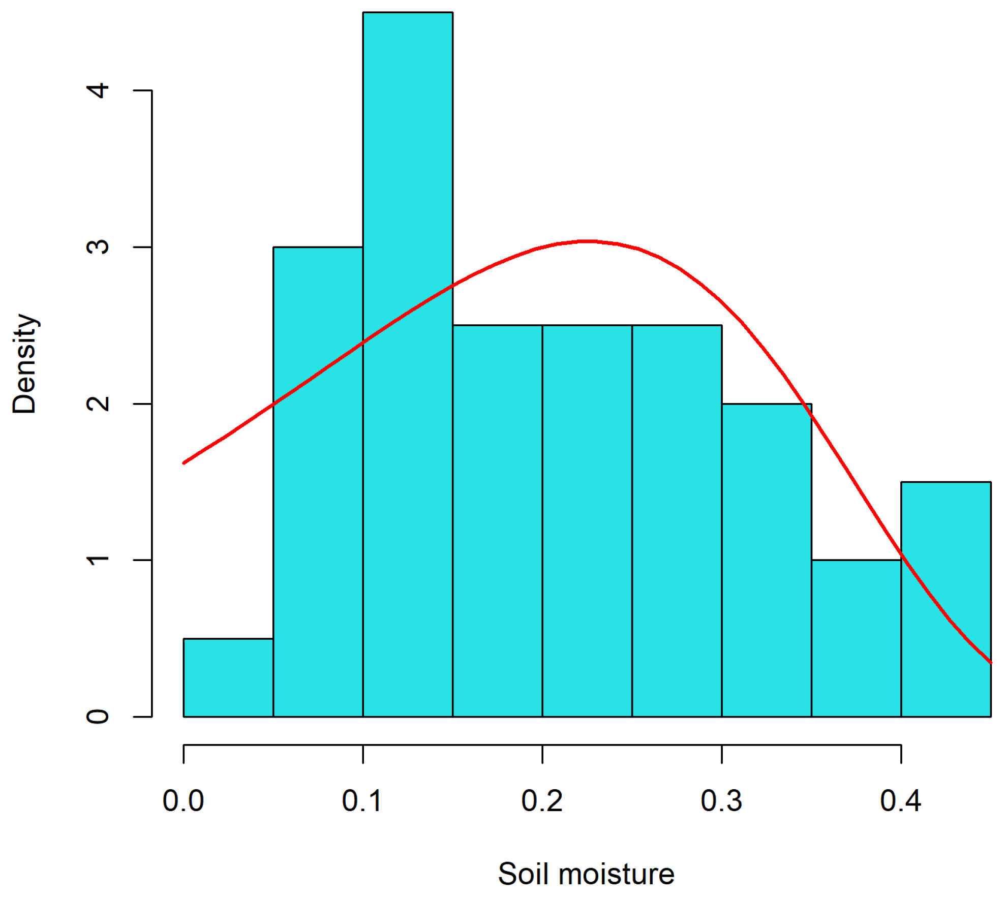
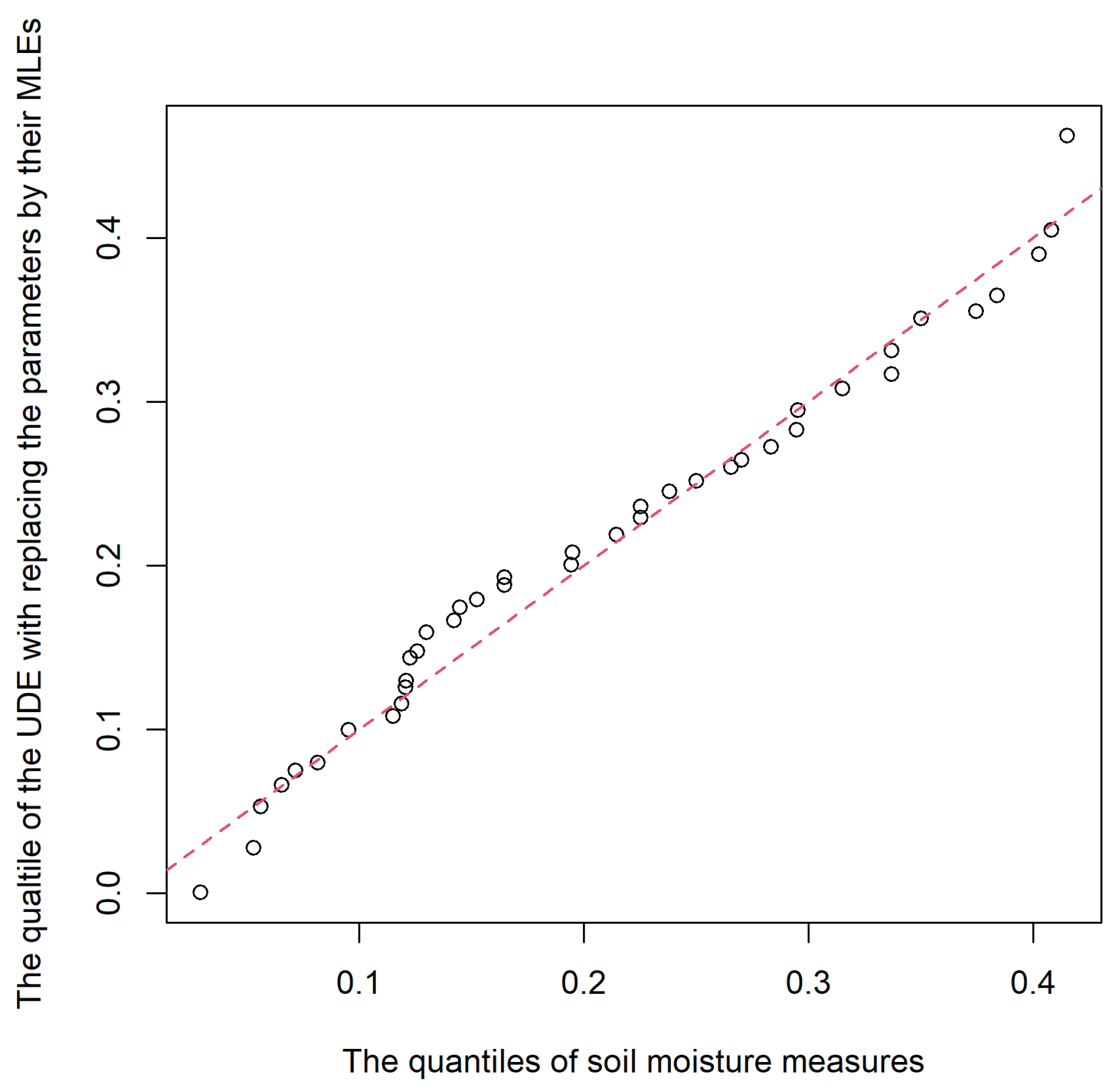
5.2. The Soil Moisture Example

The permanent wilting point indicates the threshold for plants to extract water from the soil. Plants cannot extract water from the soil when the soil moisture is below the permanent wilting point. Maity [30], page 189, reports 40 soil moisture measurements that use 0.12 as the threshold of the permanent wilting point to evaluate reliability, resilience, and vulnerability. This data set is also displaced in

Table 7. The soil moisture measurements.

0.0816	0.2253	0.1944	0.3370	0.1208	0.0954	0.0562	0.2382	0.1949	0.3500
0.4080	0.3745	0.1647	0.2654	0.1300	0.2703	0.3837	0.3152	0.1448	0.1152
0.0717	0.2253	0.4149	0.3370	0.2500	0.1423	0.1258	0.1228	0.2948	0.4024
0.2834	0.2953	0.1647	0.1190	0.0655	0.0532	0.0296	0.2145	0.1526	0.1210

for easy reference.

Using the data set shown in Table 7, the original MLEs of the UED$(\alpha ,\beta )$ parameters, $\alpha$ and $\beta$, were obtained and given in

Table 8. The MLEs and bias-corrected MLEs based on the sample of soil moisture measurements.

MLE	$\widehat{\alpha }$ = 0.2706	$\widehat{\beta }$ = 2.9962
BC	$\tilde{\alpha }$ = 0.2697	$\tilde{\beta }$ = 2.9847
Boot-BC	${\tilde{\alpha }}_{B-BC}$ = 0.2613	${\tilde{\beta }}_{B-BC}$ = 2.7608

, which provides $\widehat{\alpha }=0.2707$ and $\widehat{\beta }=2.9962$. The histogram of the soil moisture data set and the density curve of UED$(0.2707,2.9962)$ are exhibited in Figure 2. The summary statistics of the soil moisture data set are obtained by minimum = 0.0296, first quartile = 0.1210, median = 0.1946, third quartile = 0.2949, maximum = 0.4149, and mean = 0.2088, replacing $\alpha$ and $\beta$ in the UED$(\alpha ,\beta )$ by $\widehat{\alpha }$ and $\widehat{\beta }$, respectively. The quantile versus quantile plot is given in Figure 3. Using UED to model this data set, the K-S test statistics can be obtained by $D=0.125$ with the p-value = 0.6457. The K-S testing results support that the UED is the right model for the soil moisture data set.

Using the proposed bias-correction method described in Section 3.1, we can obtain the bias-corrected MLEs as $\tilde{\alpha }=0.2697$ and $\tilde{\beta }=2.9847$. Moreover, using the bootstrap bias-correction method addressed in Section 3.2 with M = 400, we obtain the B-BCML estimates as ${\tilde{\alpha }}_{B-BC}=0.2613$ and ${\tilde{\beta }}_{B-BC}=2.7608$. Both bias-corrected MLEs are smaller than the original MLEs, and the reduction magnitude of the B-BCML estimates is larger than that of the bias-corrected MLEs.

6. Conclusions

In this paper, we proposed two bias-correction procedures to reduce the bias of the MLEs of UED parameters when the sample size is small. The first bias-correction procedure is based on the bias-correction one proposed by Cordeiro and Klein [27], which has the order $O\left(n^{-2}\right)$. The second bias-correction procedure is based on the parametric bootstrap one. We analytically derived the procedure to implement the Cordeiro and Klein bias-corrected maximum likelihood estimation method. Moreover, the steps taken to obtain the bias-corrected bootstrap estimators were explored in Section 3.2.

Intensive Monte Carlo simulations were conducted to verify the performance of two bias-correction techniques. We find that the performances of the two proposed bias-correction methods are good. The computation of the Cordeiro and Klein bias-corrected maximum likelihood estimation method is simple, and the bias-corrected bootstrap estimation method is time-consuming. To demonstrate the applications of using two proposed bias-correction methods, a soil moisture data set was used for illustration.

References

1. Bayes, T. An Essay Towards Solving a Problem in the Doctrine of Chances. By the late Rev. Mr. Bayes, F.R.S. communicated by Mr. Price, in a letter to John Canton, A. M. F. R. S. Philos. Trans. R. Soc. 1763, 53, 370–418. [Google Scholar]
2. Fleiss, J.L.; Levin, B.; Paik, M.C. Statistical Methods for Rates and Proportions, 3rd ed.; John Wiley & Sons Inc.: Hoboken, NJ, USA, 1993. [Google Scholar]
3. Gilchrist, W. Statistical Modelling with Quantile Functions; CRC Press: Abingdon, UK, 2000. [Google Scholar]
4. Seber, G.A.F. Statistical Models for Proportions and Probabilities; Springer: Berlin/Heidelberg, Germany, 2013. [Google Scholar]
5. Leipnik, R.B. Distribution of the Serial Correlation Coefficient in a Circularly Correlated Universe. Ann. Math. Stat. 1947, 18, 80–87. [Google Scholar] [CrossRef]
6. Johnson, N. Systems of Frequency Curves Derived From the First Law of Laplace. Trab. Estad. 1955, 5, 283–291. [Google Scholar] [CrossRef]
7. Topp, C.W.; Leone, F.C. A Family of J-Shaped Frequency Functions. J. Am. Stat. Assoc. 1955, 50, 209–219. [Google Scholar] [CrossRef]
8. Consul, P.C.; Jain, G.C. On the Log-Gamma Distribution and Its Properties. Stat. Hefte 1971, 12, 100–106. [Google Scholar] [CrossRef]
9. Kumaraswamy, P. A Generalized Probability Density Function for Double-Bounded Random Processes. J. Hydrol. 1980, 46, 79–88. [Google Scholar] [CrossRef]
10. Jøørgensen, B. Proper Dispersion Models. Braz. J. Probab. Stat. 1997, 11, 89–128. [Google Scholar]
11. Smithson, M.; Shou, Y. CDF-Quantile. Distributions for Modelling RVs on the Unit Interval. Br. J. Math. Stat. Psychol. 2017, 70, 412–438. [Google Scholar] [CrossRef] [PubMed]
12. Altun, E.; Hamedani, G. The Log-X gamma Distribution with Inference and Application. J. Soc. Fr. Stat. 2018, 159, 40–55. [Google Scholar]
13. Nakamura, L.R.; Cerqueira, P.H.R.; Ramires, T.G.; Pescim, R.R.; Rigby, R.A.; Stasinopoulos, D.M. A New Continuous Distribution the Unit Interval Applied to Modelling the Points Ratio of Football Teams. J. Appl. Stat. 2019, 46, 416–431. [Google Scholar] [CrossRef]
14. Ghitany, M.E.; Mazucheli, J.; Menezes, A.F.B.; Alqallaf, F. The Unit-Inverse Gaussian Distribution: A New Alternative to Two-Parameter Distributions on the Unit Interval. Commun. Stat. Theory Methods. 2019, 48, 3423–3438. [Google Scholar] [CrossRef]
15. Mazucheli, J.; Menezes, A.F.; Dey, S. Unit-Gompertz Distribution with Applications. Statistica 2019, 79, 25–43. [Google Scholar]
16. Mazucheli, J.; Menezes, A.F.B.; Chakraborty, S. On the One Parameter Unit-Lindley Distribution and Its Associated Regression Model for Proportion Data. J. Appl. Stat. 2019, 46, 700–714. [Google Scholar] [CrossRef]
17. Mazucheli, J.; Menezes, A.F.B.; Fernandes, L.B.; de Oliveira, R.P.; Ghitany, M.E. The Unit-Weibull Distribution as an Alternative to the Kumaraswamy Distribution for the Modeling of Quantiles Conditional on Covariates. J. Appl. Stat. 2019, 47, 954–974. [Google Scholar] [CrossRef]
18. Altun, E. The Log-Weighted Exponential Regression Model: Alternative to the Beta Regression Model. Commun. Stat. Theory Methods 2020, 50, 2306–2321. [Google Scholar] [CrossRef]
19. Gündüz, S.; Mustafa, Ç.; Korkmaz, M.C. A New Unit Distribution Based on the Unbounded Johnson Distribution Rule: The Unit Johnson SU Distribution. Pak. J. Stat. Oper. Res. 2020, 16, 471–490. [Google Scholar] [CrossRef]
20. Biswas, A.; Chakraborty, S. A New Method for Constructing Continuous Distributions on the Unit Interval. arXiv 2021, arXiv:2101.04661. [Google Scholar]
21. Afify, A.Z.; Nassar, M.; Kumar, D.; Cordeiro, G.M. A New Unit Distribution: Properties and Applications. Electron. J. Appl. Stat. 2022, 15, 460–484. [Google Scholar]
22. Krishna, A.; Maya, R.; Chesneau, C.; Irshad, M.R. The Unit Teissier Distribution and Its Applications. Math. Comput. Appl. 2022, 27, 12. [Google Scholar] [CrossRef]
23. Korkmaz, M.Ç.; Korkmaz, Z.S. The Unit Log–log Distribution: A New Unit Distribution with Alternative Quantile Regression Modeling and Educational Measurements Applications. J. Appl. Stat. 2023, 50, 889–908. [Google Scholar] [CrossRef] [PubMed]
24. Fayomi, A.; Hassan, A.S.; Baaqeel, H.; Almetwally, E.M. Bayesian Inference and Data Analysis of the Unit–Power Burr X Distribution. Axioms 2023, 12, 297. [Google Scholar] [CrossRef]
25. Bakouch, H.S.; Hussain, T.; Tošić, M.; Stojanović, V.S.; Qarmalah, N. Unit Exponential Probability Distribution: Characterization and Applications in Environmental and Engineering Data Modeling. Mathematics 2023, 11, 4207. [Google Scholar] [CrossRef]
26. Dombi, J.; Jónás, T.; Tóth, Z.E. The Epsilon Probability Distribution and its Application in Reliability Theory. Acta Polytech. Hung. 2018, 15, 197–216. [Google Scholar]
27. Cordeiro, G.M.; Klein, R. Bias correction in ARMA models. Stat. Probab. Lett. 1994, 19, 169–176. [Google Scholar] [CrossRef]
28. Efron, B.; Tibshirani, R.J. An introduction to the bootstrap. In Monographs on Statistics and Applied Probability; Chapman & Hall: New York, NY, USA, 1993. [Google Scholar]
29. Tsai, T.-R.; Xin, H.; Fan, Y.-Y.; Lio, Y.L. Bias-Corrected Maximum Likelihood Estimation and Bayesian Inference for the Process Performance Index Using Inverse Gaussian Distribution. Stats 2022, 5, 1079–1096. [Google Scholar] [CrossRef]
30. Maity, R. Statistical Methods in Hydrology and Hydroclimatology; Springer Nature Singapore Pte Ltd.: Singapore, 2018. [Google Scholar]
Figure 1. The updated rate of the bootstrap bias-correction method for M = 200 , 300 , 400 , 500 , 600 , 700 .
Mathematics 12 01828 g001
Figure 2. The histogram of soil moisture data set and the density curve of UED ( α = 0.2707 , β = 2.9962 ) .
Mathematics 12 01828 g002
Figure 3. The quantile vs. quantile plot of the soil moisture data set versus the UED ( α = 0.2707, β = 2.9962).
Mathematics 12 01828 g003