Article

Exploring the Therapeutic Potential of Defective Interfering Particles in Reducing the Replication of SARS-CoV-2

by
Macauley Locke
1,2,†,
Dmitry Grebennikov
3,4,†,
Igor Sazonov
5,
Martín López-García
1,
Marina Loguinova
6,
Andreas Meyerhans
7,8,
Gennady Bocharov
3,9,* and
Carmen Molina-París
1,2,*
1
Department of Applied Mathematics, School of Mathematics, University of Leeds, Leeds LS2 9JT, UK
2
Theoretical Biology and Biophysics Group, Theoretical Division, Los Alamos National Laboratory, Los Alamos, NM 87545, USA
3
Marchuk Institute of Numerical Mathematics, Russian Academy of Sciences, 119333 Moscow, Russia
4
World-Class Research Center “Digital Biodesign and Personalized Healthcare”, Sechenov First Moscow State Medical University, 119991 Moscow, Russia
5
Faculty of Science and Engineering, Swansea University, Swansea SA1 8EN, UK
6
The National Medical Research Centre for Endocrinology, 117292 Moscow, Russia
7
Infection Biology Laboratory, Department of Medicine and Life Sciences (MELIS), Universitat Pompeu Fabra, 08003 Barcelona, Spain
8
Institució Catalana de Recerca i Estudis Avançats (ICREA), 08010 Barcelona, Spain
9
Institute for Computer Science and Mathematical Modelling, Sechenov First Moscow State Medical University, 119991 Moscow, Russia
*
Authors to whom correspondence should be addressed.
These authors contributed equally to this work.
Mathematics 2024, 12(12), 1904; https://doi.org/10.3390/math12121904
Submission received: 8 May 2024 / Revised: 7 June 2024 / Accepted: 13 June 2024 / Published: 19 June 2024
(This article belongs to the Special Issue Nonlinear Dynamics Research in Biomedicine)

Abstract

:
SARS-CoV-2 still presents a global threat to human health due to the continued emergence of new strains and waning immunity among vaccinated populations. Therefore, it is still relevant to investigate potential therapeutics, such as therapeutic interfering particles (TIPs). Mathematical and computational modeling are valuable tools to study viral infection dynamics for predictive analysis. Here, we expand on the previous work on SARS-CoV-2 intra-cellular replication dynamics to include defective interfering particles (DIPs) as potential therapeutic agents. We formulate a deterministic model that describes the replication of wild-type (WT) SARS-CoV-2 virus in the presence of DIPs. Sensitivity analysis of parameters to several model outputs is employed to inform us on those parameters to be carefully calibrated from experimental data. We then study the effects of co-infection on WT replication and how DIP dose perturbs the release of WT viral particles. Furthermore, we provide a stochastic formulation of the model that is compared to the deterministic one. These models could be further developed into population-level models or used to guide the development and dose of TIPs.

1. Introduction

In December 2019, a new infectious disease was reported to the World Health Organization (WHO) that would later be identified as a novel coronavirus (SARS-CoV-2) [1]. By 30 January 2020, the WHO declared SARS-CoV-2 a “public health emergency of international concern” [2], as it rapidly spread to 113 countries. By the 11th of March 2020, it had caused 118,319 infections and 4292 deaths. Consequently, the WHO declared SARS-CoV-2 a pandemic [3,4], and as of the 29 July 2022, about 572 million infections and over 6 million deaths have been recorded worldwide. During the early stages of the pandemic, treatment options were limited to chloroquine and remdesivir [5,6]. However, since then, several effective vaccines have been developed that provide protection and reduce transmission, with many countries rolling out mass vaccination programs [7]. Although vaccines for SARS-CoV-2 now exist, the emergence of new strains due to mutations has led to further concerns about vaccine effectiveness [8,9]. This fact, together with that of waning immunity and the existence of individuals who are unable to be vaccinated or out-right refuse to do so, highlight the need for additional therapeutics and prophylactics [10,11].
One such potential therapy is viral interfering particles. During viral replication, mutants lacking essential parts of the viral genome arise [12,13], which are unable to replicate in the absence of wild-type (WT) virus. These are known as defective interfering particles (DIPs). DIPs can be exploited to make therapeutic interfering particles (TIPs), which inhibit the replication of WT virus by outcompeting WT gene segments for resources required during viral replication and assembly [14,15]. TIPs/DIPs have been investigated for several viruses, including HIV, Ebola, influenza, and SARS-CoV-2, and have been found to cause a two-fold reduction in viral titres [14,15,16]. However, caveats exist in their production; for instance, which sections of the viral genome are to be removed to allow for replication at a faster rate than WT, they are virus-specific, and little is known about how mutations change replication dynamics [13,17].
From a mathematical modeling perspective, a long-standing effort exists to describe transmission dynamics at the population and within-host levels (see Ref. [18] and references therein). At the within-host level, DIPs, as therapeutics, have been studied in Refs. [19,20]. However, little effort has been devoted to investigating the intra-cellular replication kinetics of DIPs in the presence of WT virus. Grebennikov et al. [21] have recently proposed a SARS-CoV-2 intra-cellular replication dynamics model. This model allowed for the quantification of viral genomes and proteins during the replication cycle. We wish to exploit this model to explore co-infection with DIPs and the effect of DIPs on the replication dynamics of the WT virus. In particular, in this study, we formulate a mathematical model of SARS-CoV-2 replication in a cell co-infected with DIPs. As in Ref. [21], we will follow a deterministic approach to calibrate model parameters. We shall use sensitivity analysis to study the impact parameters have on the release of both WT and DIP viral particles. We also introduce a stochastic description of this model to compare to the deterministic one. We shall also investigate how initial doses of each virus affect viral particle production (WT and DIPs) to quantify DIP-related inhibition of WT replication and the reliance of DIPs on the WT replication machinery.
Overall, our study is the first one in which a detailed mathematical model (both in a deterministic and stochastic settings) of the reaction kinetics of SARS-CoV-2 life cycle in the presence of DIPs is formulated, calibrated and examined. The currently available mathematical models of SARS-CoV-2 infection dynamics considering the wild-type virus competition with the DIPs describe the within-host organism infection in upper and lower respiratory tract cells with only a single parameter characterizing the intracellular biochemical reaction cascade [15]. The high-resolution model presented below allows us to explore in detail the determinants and limits of the efficacy of DIP-based treatment of COVID-19.

2. Materials and Methods

The kinetics of the corresponding biochemical reactions are described in the deterministic mathematical model introduced in Section 3 of this paper. The system of ordinary differential equations (ODEs) is formulated under the assumption of mass action kinetics, Michaelis–Menten approximations, and on the biological scheme presented in Figure 1. The model can, in principle, be defined as a stochastic process.

2.1. Sensitivity Analysis

The mathematical model included parameters which encode the biological mechanisms under investigation. Since many parameters required calibration, it is important to identify which have the greatest effect on model outputs. Global sensitivity analysis allowed us to evaluate the results of simultaneous changes in parameter values [22,23]. For implementing this approach, consider the vector of parameters θ = ( θ 1 , θ 2 , , θ n ) such that the model output is described as Y = g ( θ ) . We use the Sobol approach to determine global sensitivities [24]. Each parameter θ i can be considered a random variable distributed uniformly on an associated range θ i [ θ i L , θ i U ] , where θ i L and θ i U are the upper and lower bounds that the parameter can take. Since Y is a function of these variables, it is also a random variable that takes values in Euclidean space with variance V ( Y ) . This total output variance can be decomposed on the sum of variances associated with the contributions of the individual parameter variations to the model output and the sum of variances associated with the interactions caused by simultaneous variations of multiple model parameters. Let E [ V ( Y | θ i ) ] be the expectation of the conditional variances V ( Y | θ i = θ i * ) (variances of Y taken over parameters θ j , j i , for a fixed θ i = θ i * ), averaged over all possible values θ i * . We were interested in how the conditional variance V ( Y | θ i = θ i * ) of the model output will change if the value of the parameter is known θ i * . The law of total variance gives [24,25]:
V ( Y ) = E [ V ( Y | θ i ) ] + V ( E [ Y | θ i ] ) ,
where the first-order Sobol sensitivity index for parameter θ i is defined as:
S i = V ( E [ Y | θ i ] ) V ( Y ) ,
where V ( E [ Y | θ i ] ) , the variance of the conditional expectation, is the main effect contribution of parameter θ i to the output variance.
We also investigated the result of multiple fixed parameter values. If we let V ( E [ Y | θ θ j ] ) be the expected reduction in the variance by fixing all parameters except θ j , then the total effect of parameter θ i can be defined as:
S T i = E [ V ( Y | θ θ i ) ] V ( Y ) = 1 V ( E [ Y | θ θ i ] ) V ( Y ) ,
where a larger sensitivity index indicates greater importance of the associated parameter to the given model output [22].

2.2. Model Development and Calibration

In formulating the new mathematical model, we introduced several additional parameters that relate to the kinetics of DIPs and the loss of non-structural proteins due to DIPs using trans-elements from the WT virus for their replication. These variables are summarized in Table 1. Grebennikov et al. provided parameter estimates for the WT virus [21]. These values are summarized in Table 2.
The remaining parameters were estimated using approximate Bayesian computation (ABC) [53]. The ABC algorithm allows a user to define a set of prior beliefs about parameter distributions, π ( θ ) , and combines this with model simulations and data to arrive at a posterior distribution π ( θ | D ) . Given a sample parameter set, θ * π ( θ ) , a user can simulate data D * π ( D | θ * ) and compare them to the experimental data, D . If the simulated data are within a given threshold distance, ε (with distance measure d ( · , · ) ), from the experimental data, D , then the sample parameter set ( θ * , D * ) is accepted. Otherwise, the parameter set is rejected and this process is continued until N parameter sets are accepted [53]. We made use of an Euclidean distance measure, defined as:
d ( M ( θ * ) , D ) = t T ( M ( θ * , t ) D ( t ) ) 2 ,
where T = { 24 , 48 } (hours) is the set of time points within the experimental dataset, D ( t ) is the observed progeny fold reduction under the treatment with DIPs at time t specified in Table 3, and M ( θ * , t ) is the respective progeny fold reduction predicted by the mathematical model. The dimensions of D and M depend on how many experimental outputs can be compared to the model outputs (both reduce to one in our case).
Datasets for defective interfering particles are limited, with little investigation of the intra-cellular replication kinetics of WT virus in the presence of DIPs. Chaturvedi et al. [15] investigated two SARS-CoV-2 DIPs as TIPs. Both DIPs had shorter genomes, around 6–10% shorter than the WT virus. Chaturvedi et al. [15] performed a virus yield-reduction assay by transfecting Vero cells with TIP or control RNAs (one μg/million cells) 24 h before infection with SARS-CoV-2 at an MOI = 0.05, and harvesting culture supernatants for titration at various time-points (24, 48, or 72 h post-infection). They discovered that these particles lead to a 1.5–1.2 log fold reduction in virus produced compared to control samples. We compared the fold reduction generated by therapeutic interfering particle two (TIP2) [15], at 24 and 48 h, to the fold reduction from our mathematical model of [ V r e l e a s e d w t ] against the original model proposed by Grebennikov et al. [21]. These fold reductions are summarized in Table 3. For the ABC rejection method, given that the choice of a suitable ε is difficult, we sampled 10 6 parameter sets and kept the top 0.1 % that minimize the distance measure d ( · , · ). We assumed uniform prior distributions for the parameters within the search ranges summarized in Table 4.

2.3. Stochastic Simulation Algorithm

To perform stochastic simulations of the model formulated as a Markov chain, the most popular exact approach is Gillespie’s direct method [54]. The Markov chain specifies the propensity a m for the m-th jump process (i.e., the respective elementary reaction rate), which changes the variables by a discrete amount when that process takes place. The propensity a m defines the probability p m = a m d t that the m-th process is triggered in the infinitesimal time interval [ t , t + d t ) . At each step of the simulation, two random numbers r 1 , r 2 U ( 0 , 1 ) are generated to sample the time of the next jump process, τ , and the index r m of the process to perform:
τ = 1 a 0 log ( 1 / r 1 ) , r m = arg min μ m = 1 μ a m r 2 a 0 ,
where a 0 = m = 1 M a m is the total sum of propensities.
In this work, we used the rejection stochastic simulation algorithm (RSSA) [55]. This method estimates the upper and lower bounds on the propensities a m ̲ ,   a m ¯ , instead of calculating the exact values, a m , and uses the third random number, r 3 U ( 0 , 1 ) , for a rejection test to check if the exact value is needed to be computed (see details in Ref. [55]). The propensity values are updated only when necessary; therefore, the algorithm is practical when the propensity computation is time-consuming, e.g., for non-linear process rates parameterized with Michaelis–Menten functions. Additionally, two dependency graph structures are defined to reduce the number of propensity updates and accelerate computations: the first one specifies for each process which variables are affected when the corresponding jumps occur, and the second one specifies for each variable the process indices with propensities dependent on the value of the variable. Note that certain search strategies for the candidate process can also be implemented (e.g., RSSA with composition–rejection search (RSSA-CR) groups the jump processes by their propensity bounds). Alternatively, one can use approximate methods to significantly speed up computations, such as the tau-leaping method [54], or the other hybrid methods that make use of SDE or ODE approximations [55,56]. In this work, however, we used the exact RSSA method, as the performance of the parallelized code to compute the ensemble of stochastic trajectories was acceptable.

2.4. Software

The following packages in Python language (version 3.8.8) were used to simulate and analyze the model: Scipy (version 1.8.1) to numerically solve the system of ordinary differential equations, SALib (version 1.4.5) for identification of Sobol sensitivity indices, Matplotlib (version 3.5.1) for visualizations, and Joblib (version 1.0.1) for parallelization of the ABC rejection algorithm, which allows to infer posterior distributions of model parameters. To perform stochastic simulations, we used the package DifferentialEquations.jl (version 7.4.0) in Julia language (version 1.8.1). Codes used to simulate and analyze these models are available in the GitHub repository https://github.com/MacauleyLockeml/SARS-CoV-2-DIP-Model (accessed on 12 June 2024).

3. Mathematical Model of WT and DIP Infection

The variables of the mathematical model characterizing the life cycle of SARS-CoV-2 according to Figure 1 are listed in Table 1. The unknown functions [ · ] characterizing the abundance of the constituents of the SARS-CoV-2 replication system are the time-dependent variables with their rates of change in time described by the system of the ordinary differential equations introduced below. The parameters (coefficients) appearing on the right-hand side of the equations are the rate constants of the processes specified in Table 2 and Table 4.

3.1. Cell Entry and RNA Release

The binding of infectious WT virion to the cellular trans-membrane protein ACE2 allows entry and release of the viral RNA into the host cell. We describe this process by equations specifying the rates of change of free-, receptor-bound, and fused virions, as well as the viral RNA genome in the cytoplasm:
d [ V f r e e w t ] d t = k b i n d [ V f r e e w t ] d V w t [ V f r e e w t ] + k d i s s [ V b o u n d w t ] ,
d [ V b o u n d w t ] d t = k b i n d [ V f r e e w t ] ( k f u s e + k d i s s + d V w t ) [ V b o u n d w t ] ,
d [ V e n d o s o m e w t ] d t = k f u s e [ V b o u n d w t ] ( k u n c o a t + d e n d o s o m e w t ) [ V e n d o s o m e w t ] ,
d [ g R N A ( + ) w t ] d t = k u n c o a t [ V e n d o s o m e w t ] d g R N A w t [ g R N A ( + ) w t ] .
where [ V f r e e w t ] is the number of extra-cellular free infectious virions, [ V b o u n d w t ] is the number of virions bound to ACE2 and activated by TMPRSS2, [ V e n d o s o m e w t ] is the number of virions in endosomes, and [ g R N A ( + ) w t ] is the number of ss-positive sense genomic RNA. A similar set of equations is used to describe the cell entry and RNA release of non-infectious viral defective interfering particles:
d [ V f r e e d i p ] d t = k b i n d [ V f r e e d i p ] d V d i p [ V f r e e d i p ] + k d i s s [ V b o u n d d i p ] ,
d [ V b o u n d d i p ] d t = k b i n d [ V f r e e d i p ] ( k f u s e + k d i s s + d V d i p ) [ V b o u n d d i p ] ,
d [ V e n d o s o m e d i p ] d t = k f u s e [ V b o u n d d i p ] ( k u n c o a t + d e n d o s o m e d i p ) [ V e n d o s o m e d i p ] ,
d [ g R N A ( + ) d i p ] d t = k u n c o a t [ V e n d o s o m e d i p ] d g R N A d i p [ g R N A ( + ) d i p ] .
where [ V f r e e d i p ] is the number of extra-cellular free DIPs, [ V b o u n d d i p ] is the number of DIPs bound to ACE2 and activated by TMPRSS2, [ V e n d o s o m e d i p ] is the number of DIPs in endosomes, and [ g R N A ( + ) d i p ] is the number of ss-positive sense genomic RNA. DIPs for SARS-CoV-2 would require a functional spike (S) protein to successfully bind to ACE2 receptors and mediate cell entry. Consequently, we assume that the rates for k b i n d , k d i s s , k f u s e , and k u n c o a t are the same for both WT virus and DIPs. However, degradation rates related to cell entry will differ between WT and DIPs, since the shorter genome of DIPs might imply a different degradation rate.

3.2. RNA Transcription and DIP Parasitism

The released WT viral genomic RNA undergoes translation into non-structural viral polyproteins, [ N S P ] , which operate to form the viral replication and transcription complex, i.e., the RNA-dependent RNA polymerase (RdRp). The main function of the RdRp replication complex is to generate a negative sense full-length genomic and subgenomic RNAs. As DIPs lack the ability of self-replication, the conditional transcription of DIP RNAs results in competition with WT SARS-CoV-2 for replication proteins [15]. The use of WT virus t r a n s elements by DIPs reduces [ N S P ] availability for the transcription of WT viral RNA. The respective sets of equations have different structures, as detailed below. The abundance of non-structural proteins, [ N S P ] , the negative sense genomic and subgenomic RNAs, [ g R N A ( ) w t ] , and positive sense genomic and subgenomic RNAs, [ g R N A w t ] , associated with the replication of the infectious virions are described by the following equations:
d [ N S P ] d t = k t r a n s l f O R F 1 [ g R N A ( + ) w t ] d N S P [ N S P ] ( k t r a n s ( ) w t [ g R N A ( + ) w t ] + k t r a n s ( + ) w t [ g R N A ( ) w t ] + k t r a n s ( ) d i p [ g R N A ( + ) d i p ] + k t r a n s ( + ) d i p [ g R N A ( ) d i p ] ) [ N S P ] ,
d [ g R N A ( ) w t ] d t = k t r ( ) w t [ g R N A ( + ) w t ] θ R d R p d g R N A ( ) w t [ g R N A ( ) w t ] ,
d [ g R N A w t ] d t = k t r ( + ) w t [ g R N A ( ) w t ] θ R d R p ( k c o m p l e x w t θ c o m p l e x + d g R N A w t ) [ g R N A w t ] ,
where
θ R d R p = [ N S P ] [ N S P ] + K N S P , θ c o m p l e x = [ N ] [ N ] + K N .
Equation (12) reflects the fact that non-structural proteins are translated only from the viral genomic RNA of infectious WT virions. Transcription of negative sense viral genomic and subgenomic RNAs described by Equations (13) and (14) is regulated by the positive sense viral genomic RNA. The set of equations for transcription of negative sense and positive sense DIP subgenomic RNAs, i.e., [ g R N A ( ) d i p ] , [ g R N A d i p ] are as follows:
d [ g R N A ( ) d i p ] d t = k t r ( ) d i p [ g R N A ( + ) d i p ] θ R d R p d g R N A ( ) d i p [ g R N A ( ) d i p ] ,
d [ g R N A d i p ] d t = k t r ( + ) d i p [ g R N A ( ) d i p ] θ R d R p ( k c o m p l e x d i p θ c o m p l e x + d g R N A d i p ) [ g R N A d i p ] .

3.3. Translation and Competition for Nucleocapsid Protein and Other Structural Proteins

DIPs compete with WT virions for packaging proteins, e.g., nucleocapsid N proteins ( [ N ] ) [15]. Structural S, envelope E, and membrane M proteins are translated from positive sense subgenomic RNAs in the endoplasmic reticulum (ER) and are considered in the mathematical model as a single population, [ S P ] . Nucleocapsid proteins, on the other hand, are translated in cytosolic ribosomes from positive sense RNAs. Both S P and N proteins are required for the formation of virus like-particles, WT or DIPs. It can be assumed that n S P d i p n S P w t and n N d i p n N w t , since the shorter DIP genome will require fewer N proteins for the formation of the ribonucleocapsid and construction of a viral particle. Translation of N and S P proteins are described by the following two equations:
d [ N ] d t = k t r a n s l f N [ g R N A w t ] k c o m p l e x w t n N w t θ c o m p l e x [ g R N A w t ] k c o m p l e x d i p n N d i p θ c o m p l e x [ g R N A d i p ] d N [ N ] ,
d [ S P ] d t = k t r a n s l f S P [ g R N A w t ] k a s s e m b w t n S P w t θ a s s e m b w t [ N - g R N A w t ] k a s s e m b d i p n S P d i p θ a s s e m b d i p [ N - g R N A d i p ] d S P [ S P ] ,
where
θ a s s e m b w t = [ S P ] [ S P ] + K V rel w t n S P w t ,
and
θ a s s e m b d i p = [ S P ] [ S P ] + K V rel d i p n S P d i p ,

3.4. Assembly and Release of WT SARS-CoV-2 and DIPs

New virions are assembled at the endoplasmic reticulum–Golgi compartment, where N-RNA complexes become encapsulated. These assembled virions can then exit an infected cell by exocytosis via the lysosomal pathway, budding, or cell death [57,58]. There is no competition associated with the release of new infectious and DIP virions, but the viral assembly rates, θ a s s e m b w t and θ a s s e m b d i p , depend on the availability of structural proteins, since DIPs will likely require fewer of them than WT virions. The rates of change of the ribonucleocapsid and assembled and released infectious SARS-CoV-2 and DIPs are described below:
d [ N - g R N A w t ] d t = k c o m p l e x w t θ c o m p l e x [ g R N A w t ] ( k a s s e m b w t θ a s s e m b w t + d N - g R N A w t ) [ N - g R N A w t ] ,
d [ V a s s e m b l e d w t ] d t = k a s s e m b w t θ a s s e m b w t [ N - g R N A w t ] ( k r e l e a s e w t + d a s s e m b l e d w t ) [ V a s s e m b l e d w t ] ,
d [ V r e l e a s e d w t ] d t = k r e l e a s e w t [ V a s s e m b l e d w t ] d V w t [ V r e l e a s e d w t ] ,
and
d [ N - g R N A d i p ] d t = k c o m p l e x d i p θ c o m p l e x [ g R N A d i p ] ( k a s s e m b d i p θ a s s e m b d i p + d N - g R N A d i p ) [ N - g R N A d i p ] ,
d [ V a s s e m b l e d d i p ] d t = k a s s e m b d i p θ a s s e m b d i p [ N - g R N A d i p ] ( k r e l e a s e d i p + d a s s e m b l e d d i p ) [ V a s s e m b l e d d i p ] ,
d [ V r e l e a s e d d i p ] d t = k r e l e a s e d i p [ V a s s e m b l e d d i p ] d V d i p [ V r e l e a s e d d i p ] .
In this study, we wish to explore model behaviour for different initial conditions, [ V f r e e w t ] ( 0 ) and [ V f r e e d i p ] ( 0 ) , and thus, understand the replication dynamics of WT viral particles in the presence of DIPs, and how the initial dose of WT or DIP particles regulates infection and production kinetics of WT virions. We are also interested in investigating the sensitivities to model parameters of different outputs.
The deterministic model specified by the set of equations Equations (4)–(27) represents a bounded rate system. Modeling of SARS-CoV-2 replication dynamics amounts to solving an initial value problem, which describes the system evolution with time for the given initial conditions of the system.

3.5. Stochastic Markov Chain Model

The deterministic model defined by Equations (4)–(27) can be generalized to a stochastic one formulated as a discrete-state continuous-time Markov chain (DSCT MC). The stochastic model allows one to account for integer-valued variables, to obtain probability distributions rather than mean field estimates for the variables of interest, and to compute the probabilities of productive cell infection at low MOI [59]. It is convenient to estimate model parameters for the system of ODEs and then, with a calibrated deterministic system and a defined Markov chain model, perform stochastic simulations making use of Monte Carlo methods. We follow our previous effort on the stochastic modeling of SARS-CoV-2 [59] and HIV-1 [56] life cycles to formulate and simulate the Markov chain. The Markov chain corresponding to Equations (4)–(27) is presented in Table 5. It includes the state transition events and the propensities, a m , for the m-th jump process. The propensity a m defines the probability p m = a m d t that the m-th process takes place in the infinitesimal time interval [ t , t + d t ) . This definition yields exponential distributions for the time between jumps and various Monte Carlo methods can be used to simulate the stochastic trajectories from these distributions [54,55]. We note that the processes of ribonucleocapsid formation ( m = 33 , 34 ) and virion assembly ( m = 37 , 38 ) are formulated as single events, yet involve the simultaneous change of three different variables. In these processes, protein copy numbers are decreased by the corresponding number of protein molecules, n p , needed to form a complex or assemble a pre-virion particle (i.e., by n N w t , n N d i p , n S P w t , or n S P d i p , respectively). Alternatively, one can formulate the Markov chain (MC) with three separate processes for each assembly event, in which the protein molecules are decreased by only one molecule with the propensity multiplied by n p (see Ref. [59] for an example of the extended MC formulation). We have verified that the extended and reduced MCs produce similar statistics. This reduction can be viewed as a weighted sampling strategy used in probability-weighted dynamic Monte Carlo method (PW-DMC) to accelerate computations [55].

4. Results

4.1. Sensitivity Analysis

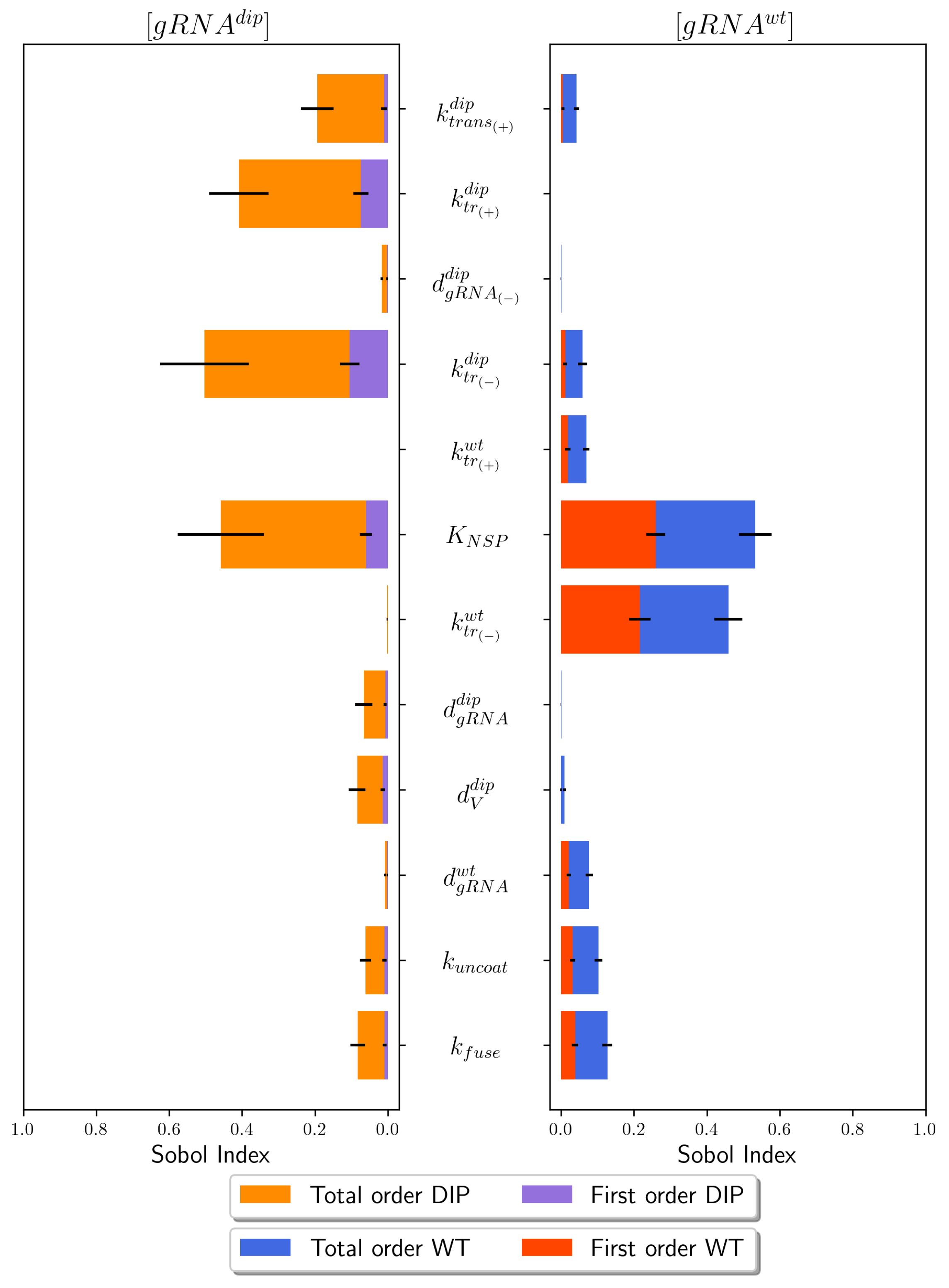
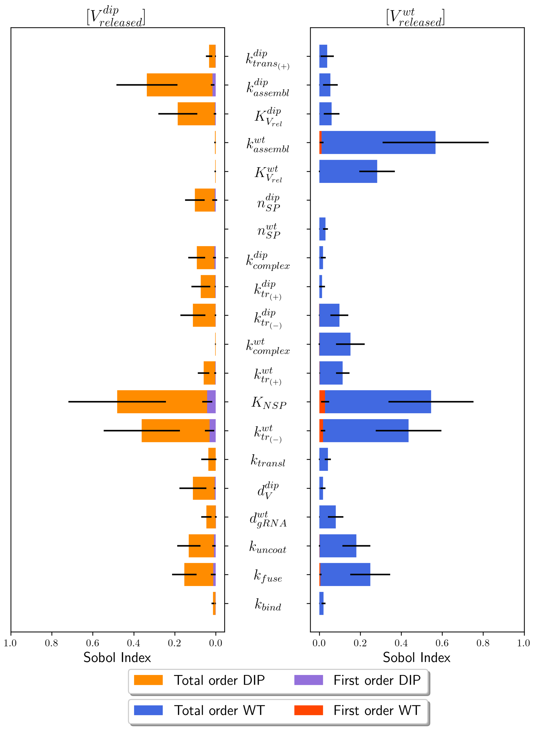
We now evaluate how model outputs change with parameter values. To that end, a Sobol global sensitivity analysis was performed on four different model outputs. We first considered the variability of WT genomic RNA, [ g R N A w t ] , and DIP genomic RNA, [ g R N A d i p ] , as a result of modifying parameter values within a set range summarized in Table 2 and Table 4. Secondly, we investigated how parameter variability affects the release kinetics of both WT [ V r e l e a s e d w t ] and DIP [ V r e l e a s e d d i p ] particles 48 h post-infection. These are illustrated in Figure 2 and Figure 3. Understanding which parameters cause the most variability in our model will allow us to calibrate it with careful consideration to minimize output perturbations.
Figure 2 illustrates the first- and total-order sensitivities for WT genomic RNA, [ g R N A w t ] , and DIP genomic RNA, [ g R N A d i p ] , as outputs of the proposed model. For [ g R N A d i p ] , the parameter k t r ( ) d i p was identified as generating the largest variation. k t r ( ) d i p is associated with the transcription of negative sense RNAs for DIPs, and thus, it is essential in the formation of new positive sense genomic and subgenomic RNAs. The rate k t r ( + ) d i p was also identified as a high sensitivity parameter, since it is associated with the transcription of positive sense RNAs. Consequently, k t r ( ) w t was the second most important parameter in minimizing variation in model output for [ g R N A w t ] , following the same reasoning as for DIP positive sense genomic RNA.
A parameter that was of great importance, and not only caused large variation in model outputs of [ g R N A   ] for WT or DIPs, but also [ V r e l e a s e d   ] (Figure 3) was the threshold parameter of non-structural proteins, K N S P . K N S P causes the most variation for [ V r e l e a s e d d i p ] and [ g R N A w t ] compared to any other parameter, and for [ V r e l e a s e d w t ] and [ g R N A d i p ] , it is the second most important parameter. K N S P is associated with the transcription of both negative and positive sense genomic RNAs, and changes in the value of this parameter will modify the number of WT virions and DIPs released. k t r ( ) w t was identified as an important parameter to minimize variation in the release of both WT [ V r e l e a s e d w t ] and DIPs [ V r e l e a s e d d i p ] . Consequently, transcription of negative sense WT genomic RNAs is an essential first step in producing positive stranded gRNA, which is then translated to form structural proteins S, M, and E ( [ S P ] ), as well as nucleocapsid proteins ( [ N ] ), which are required to form new viral particles. Parameters associated with WT virion or DIP assembly are also important to monitor to reduce variation in model outputs. Several of the parameters identified by the Sobol sensitivity analysis have been previously estimated in Ref. [21] and are summarized in Table 2. Other parameters required estimation and these are listed in Table 4.

4.2. Parameter Calibration

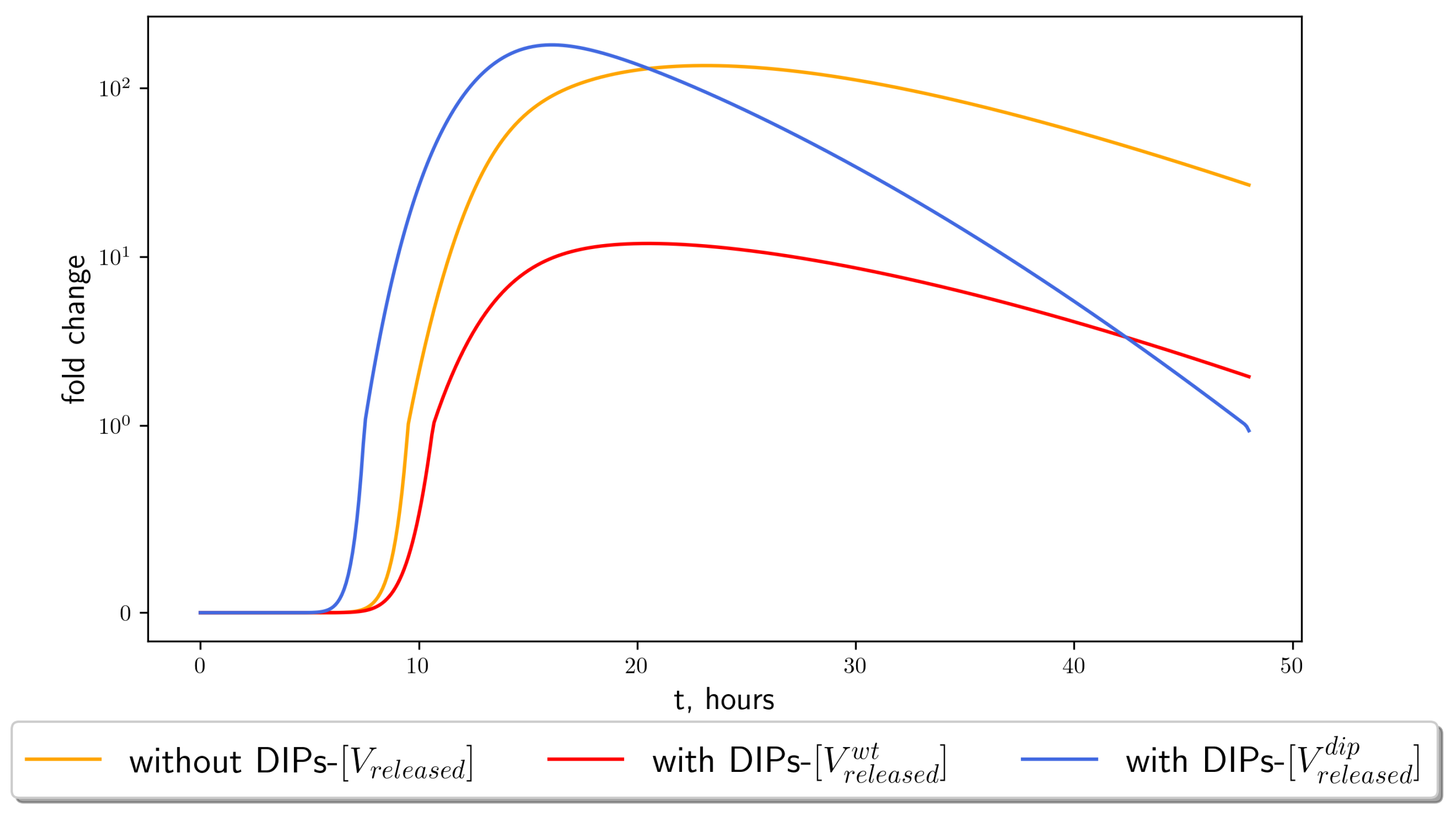
In our extension of the model proposed by Grebennikov et al. in Ref. [21], we introduced several parameters which have not been previously quantified. To estimate their values, we performed Bayesian parameter calibration. Since experimental datasets on co-infection with DIPs is limited, we aimed to achieve the fold reduction experimentally quantified by Chaturvedi et al. in Ref. [15]. We made use of an ABC rejection algorithm with 10 6 sample sets. As previously mentioned, since a choice of ε is hard to determine, we instead took the 0.1 % of parameter sets which minimize the Euclidean distance. We sampled the exponent of the search ranges shown in Table 4. As a result, our sample size provided a large coverage of parameter space. We compared the fold log reduction between the reference solution of a model without DIPs and the one with DIPS to the data in Table 3, and Figure 4 illustrates the model output where we used the median values from the accepted 0.1 % sample sets. From these median values, we obtained a fold change of 1.08 (two d.p.) at 24 h post-infection and 1.14 (two d.p.) at 48 h post-infection, compared to the reference solution [21]. Posterior histograms in Figure A1 showed that with the dataset and the mathematical model, Bayesian inference has led to poor learning for all but one of the newly introduced parameters. Posterior distributions are still extremely wide, with k t r a n s ( + ) w t being the only parameter with a narrow posterior distribution. This was due to lack of longitudinal data to compare modeled DIP replication dynamics with.
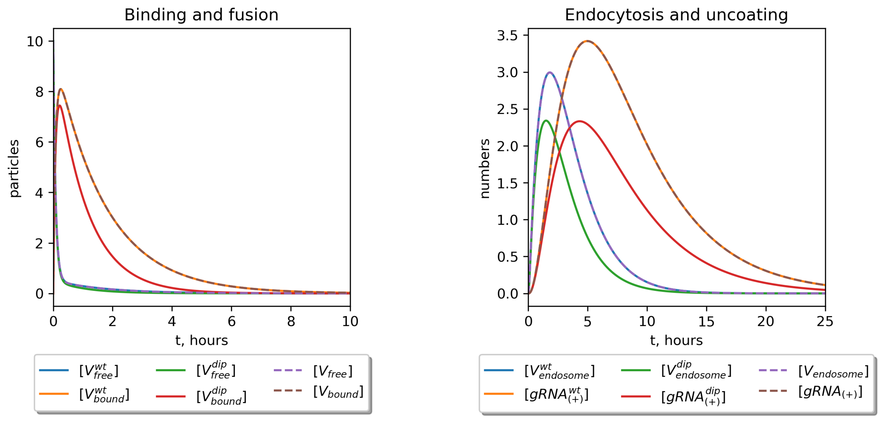
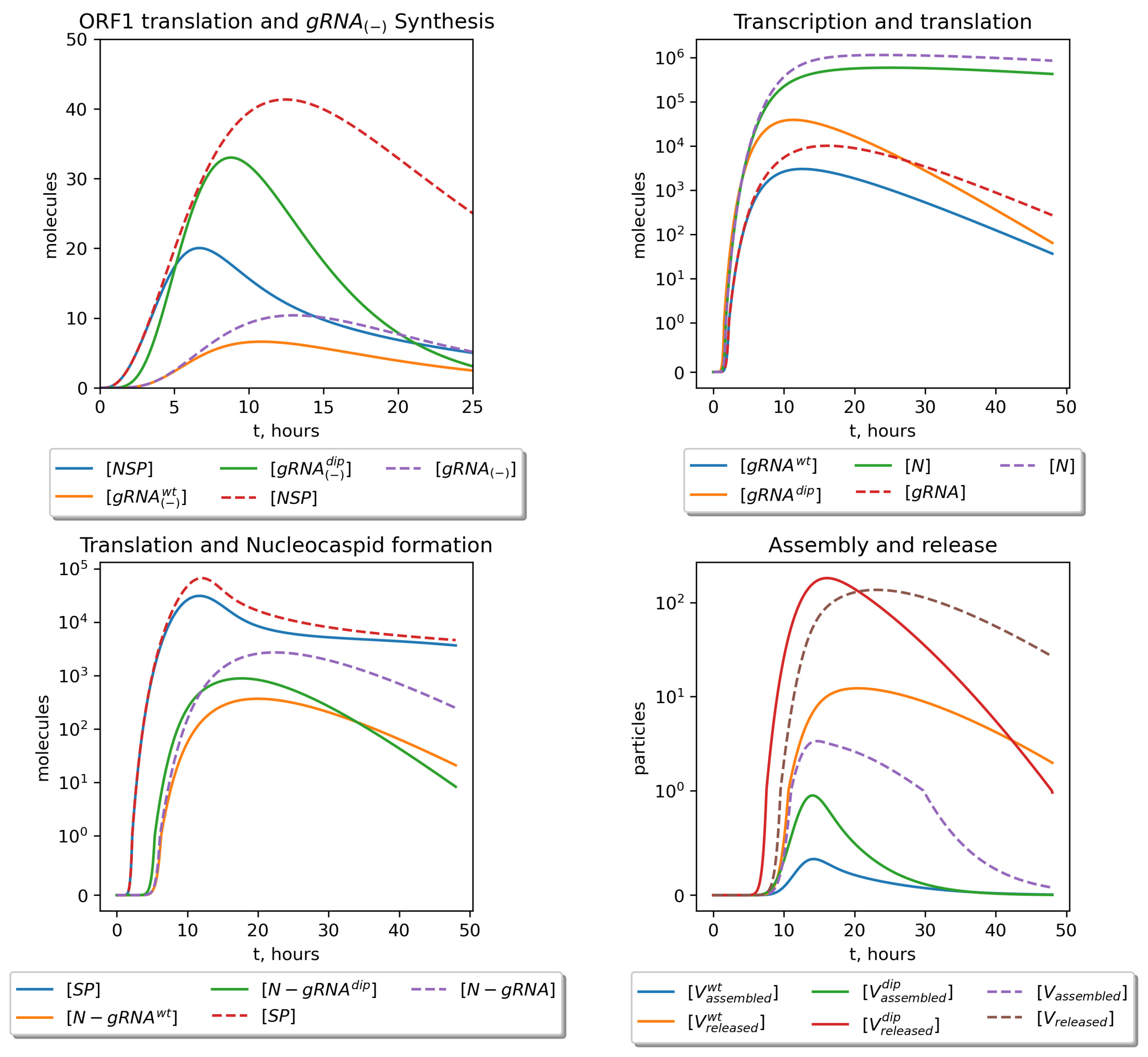
Figure 5 illustrates the time evolution for each variable in Table 1 given the median values found via ABC rejection. From the upper panels of Figure 5, we examined that the entry kinetics of WT virus into the cell are similar to those of the reference solution. DIPs, however, enter the cell at a faster rate than WT virions. It is important to remember that we assumed there are sufficient ACE2 receptors mediating viral entry; thus, there is no competition between WT and DIP for receptor binding. The number of non-structural proteins is greatly reduced (Figure 5 middle left panel), peaking at 7 h with ≈20 molecules as opposed to the reference solution, which peaks at roughly 13 h with ≈40 molecules. The production of [ g R N A ( ) w t ] halves and peaks earlier in the time course, with a greater number of DIP negative sense genomic RNA than WT. Consequently, we then saw an approximate fold reduction of positive sense genomic RNA, ribonucleocapsid proteins, and assembled and released WT viral particles.

4.3. Stochastic Model Results

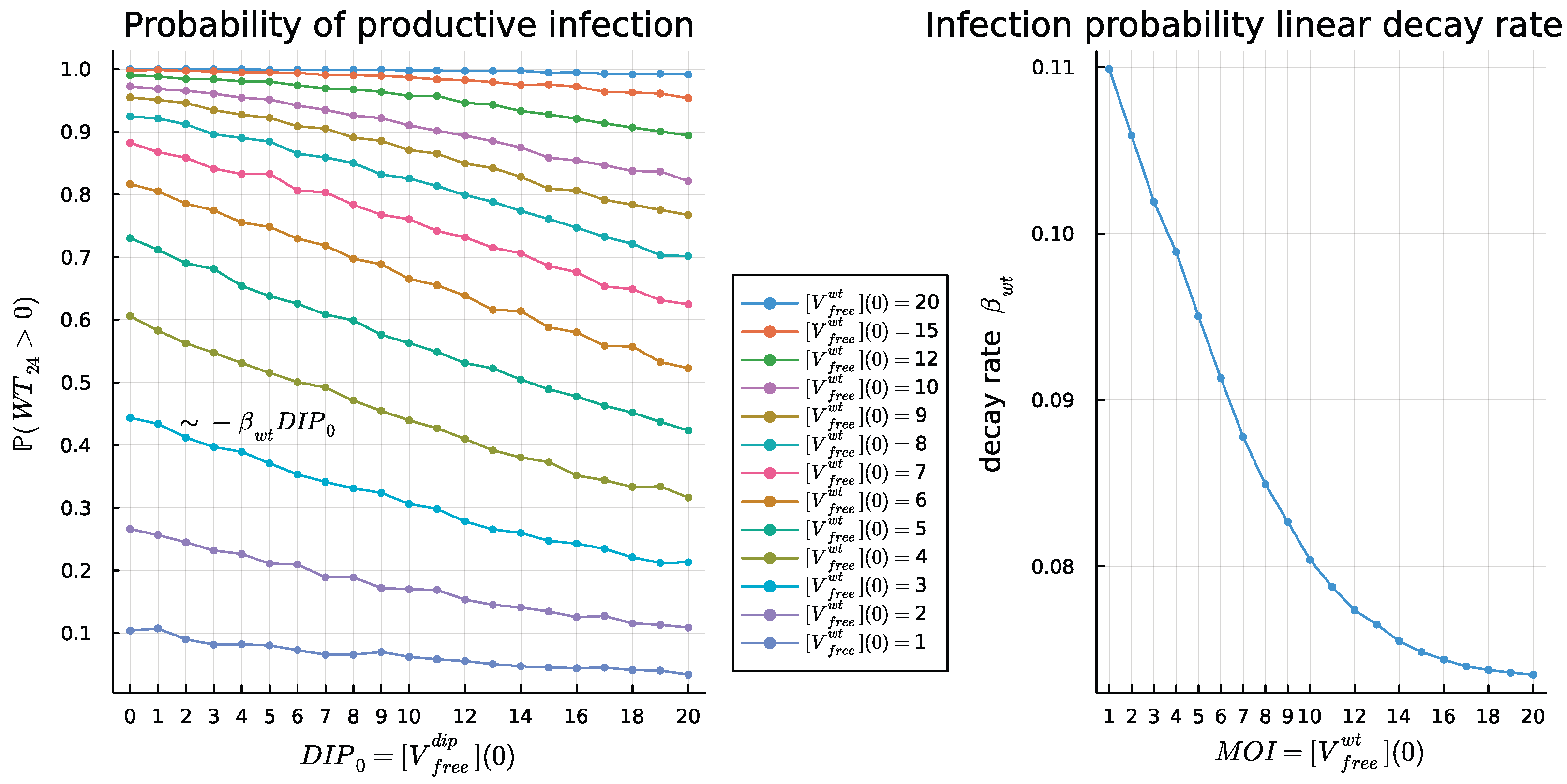
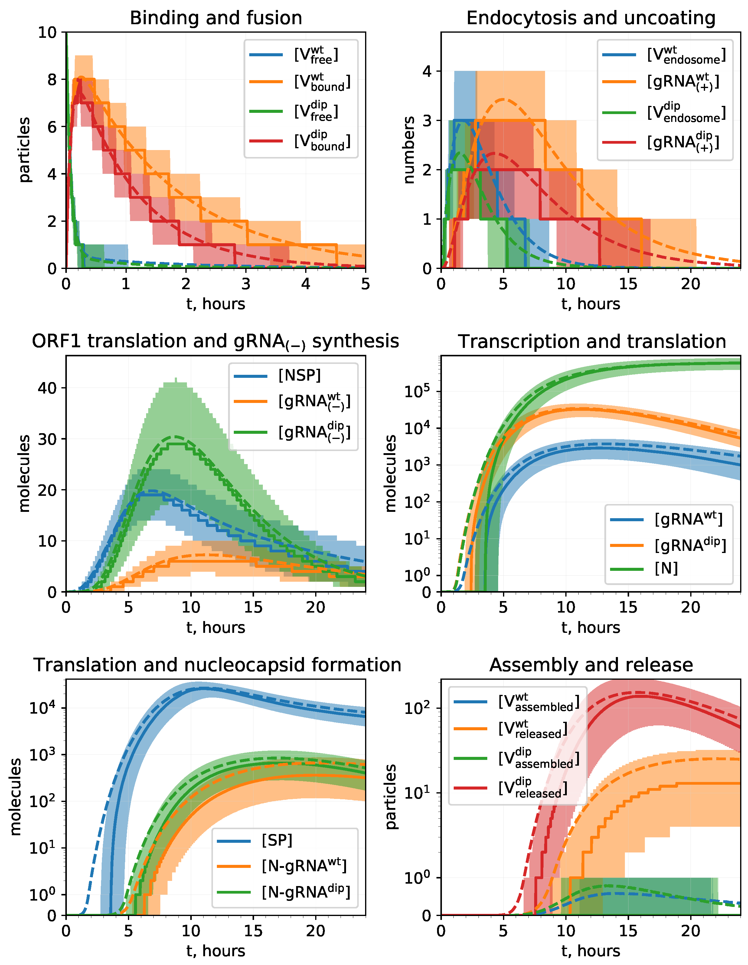
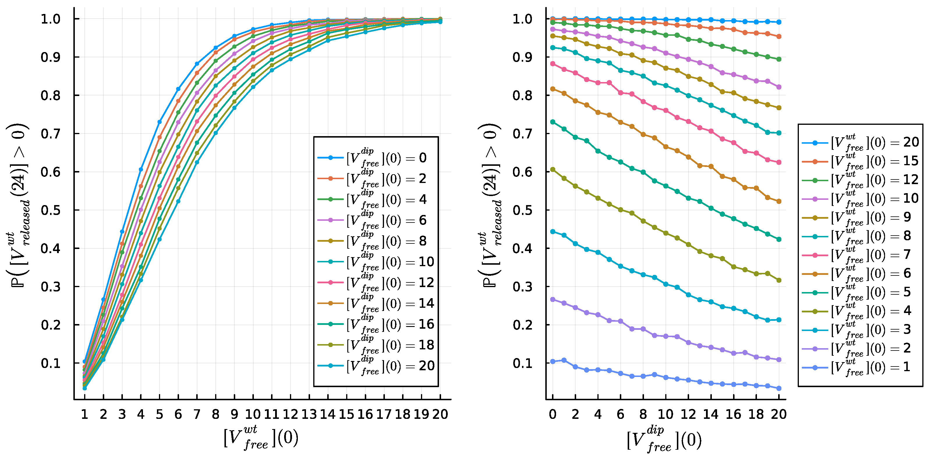
Figure 6 shows the kinetics of the stochastic model variables for initial doses of wild-type virus [ V f r e e w t ] ( 0 ) = 10 and DIPs [ V f r e e d i p ] ( 0 ) = 10 . The figure illustrates parametric (mean values) and non-parametric (medians, inter-quartile ranges) statistics computed on an ensemble of 10 6 trajectories. Additionally, the histograms of the simulated variable values at particular time points can be produced from the ensemble for analysis (Figure A2). The means and medians follow approximately the deterministic model outputs, while the inter-quartile ranges estimate the uncertainty of the simulations due to stochastic effects caused by the discrete nature of the model variables. These stochastic effects are more prominent for variables which are present in a cell in small numbers, and the assumption that their mean values can be approximated by the deterministic model may not be satisfied. In particular, the deterministic model predicts that an infection is productive for every positive initial dose of [ V f r e e w t ] ( 0 ) = 10 , while the stochastic trajectories can become extinct due to stochasticity. Figure 7 illustrates the probability of productive infection as a function of the initial WT virion (MOI) and DIP doses. As can be seen in Figure 7 (left panel), the probability of a productive infection tends to one as the initial dose of the WT virus hits 20 viral particles. However, the probability is affected by the initial dose of DIP particles (Figure 7, right panel), with this probability being reduced linearly as the dose increases.
The mean values of WT virion and DIP production 24 h post-infection closely follow the outputs predicted by the deterministic model. However, a part of the trajectories simulated with the stochastic model become extinct. The probability of productive infection as a function of WT M O I and D I P 0 is shown in Figure 7. When this probability is close to one, a change in D I P 0 does not significantly modify it. For every WT M O I , an increase in DIP dose reduces this probability linearly. Figure A5 shows the dependence of this linear decay in probability, β w t , on WT M O I .

4.4. Dose Response Analysis

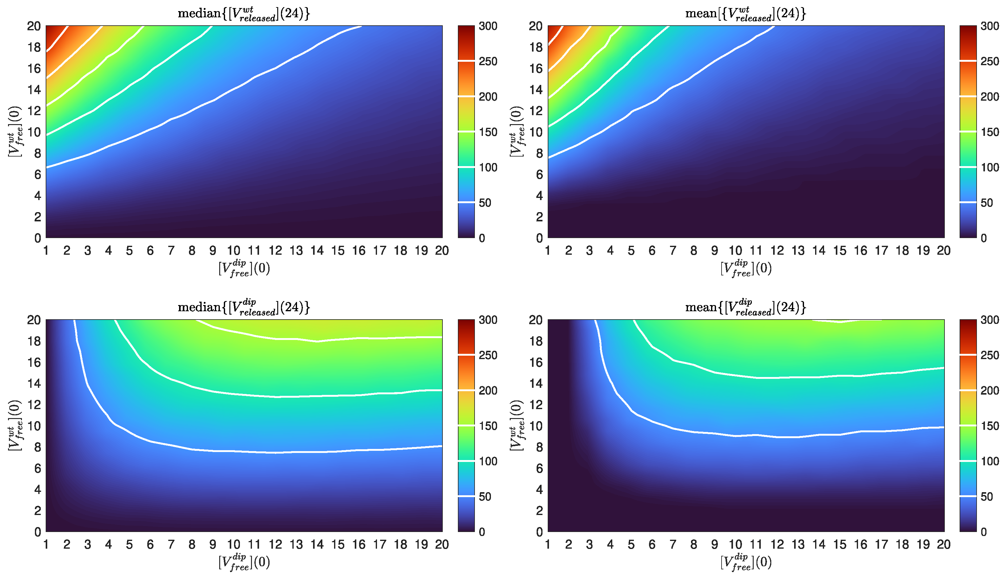
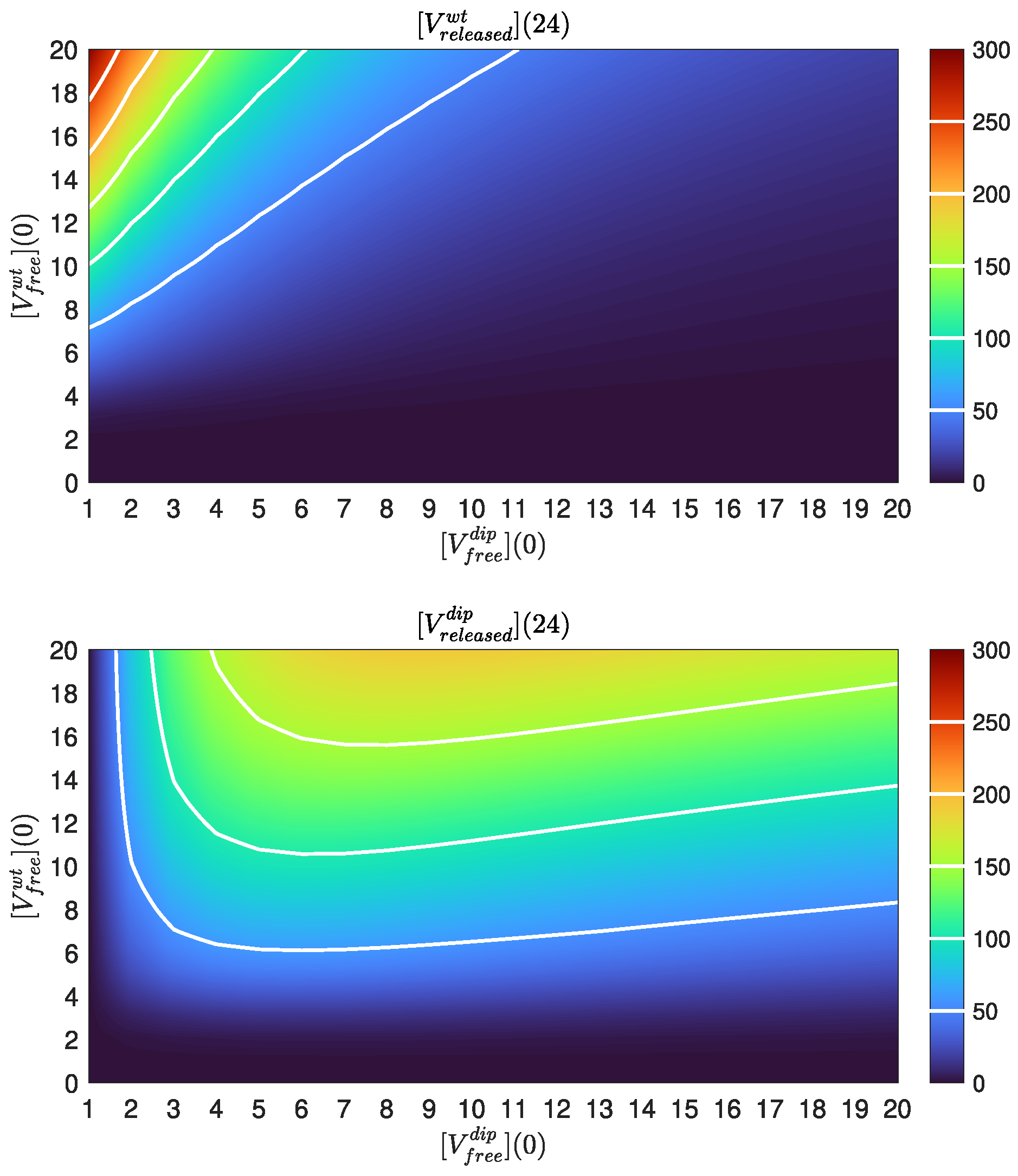
We examined the release kinetics, i.e., the abundance of WT virions compared to DIPs, as a function of the initial doses [ V f r e e w t ] ( 0 ) = [ V f r e e d i p ] ( 0 ) = 10 . However, one can expect that initial infection doses might vary from cell to cell. Therefore, we now examined the release kinetics of WT virions under different initial conditions. Figure 8 illustrates the total number of WT virions (left) and DIPs (right) released with initial conditions [ V f r e e w t ] ( 0 ) = 1 –20 and [ V f r e e d i p ] ( 0 ) = 1 –20 over a 24 h time period. As can be seen from Figure 8, a low dose of DIPs (MOI = 1 ) with a high dose of WT virus (MOI = 20 ) results in an approximately 21% reduction of the WT particles released during DIP co-infection. Furthermore, as we decreased the initial number of WT virions while DIPs remained at an MOI = 1 , we observed a continued decrease in WT virus released during co-infection compared to the single infection case (no DIPs). As the dose of DIPs was increased, the total number of WT virions released rapidly decreased, and at MOI = 10 for WT and DIP MOI = 4 WT particles only account for approximately 30 % of particles released. These deterministic results were consistent with median estimates from the stochastic model presented in Figure A3 (upper panel), while the mean estimates (Figure A3, lower panel) showed marginally higher release in WT virus and lower release of DIPs. Additionally, for high doses of WT virus, a productive infection is almost guaranteed (Figure 7), but as shown in Figure A3, even if an infection is guaranteed the overall number of WT, and hence infectious particles, is reduced.
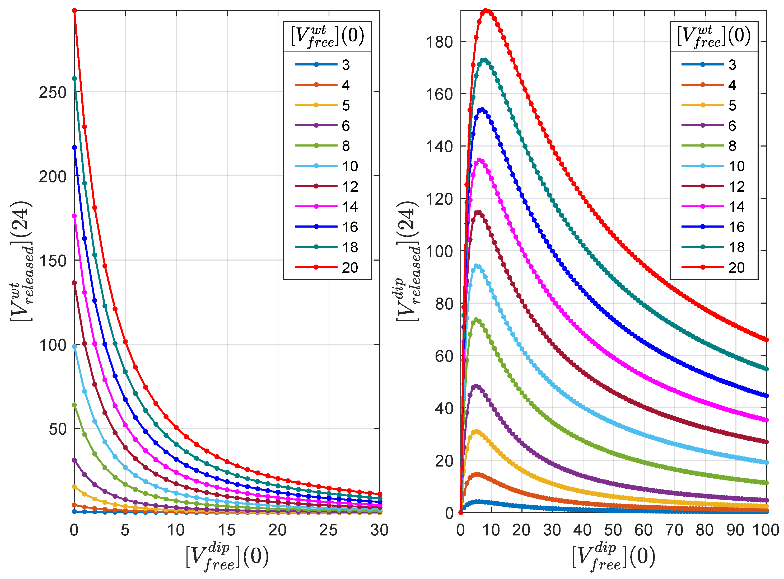
Figure 9 shows viral particle release kinetics predicted by the deterministic model with fixed initial conditions for [ V f r e e w t ] ( 0 ) ranging from 3 to 20 virions and varying initial conditions for DIPs [ V f r e e d i p ] ( 0 ) = 1–100. DIP release peaks at a MOI = 6 and then begins to decrease as the dose increases. An increase in dose continues to have an effect on the release of WT virions, so that for a MOI = 40 , total WT virion production is <30 virions released over the 24 h time period considered. This highlights the ability of DIPs to compete (with an advantage) for replication resources with WT virions. Consequently, if the dose is high enough, DIPs sequester so many intra-cellular resources that WT production is significantly reduced. Finally, the non-linear effects of DIP MOI on WT virion and DIP production per cell suggest that there might be optimal dosing of DIPs when used as a therapeutic agent. The maximum effect can potentially be achieved at around 5 to 10 DIPs per cell as this would maximize the number of new DIPs produced by the infected cells, and these, in turn, will reduce the WT virion production in other infected bystander cells.

4.5. DIP Dose Effect on WT Virion Production

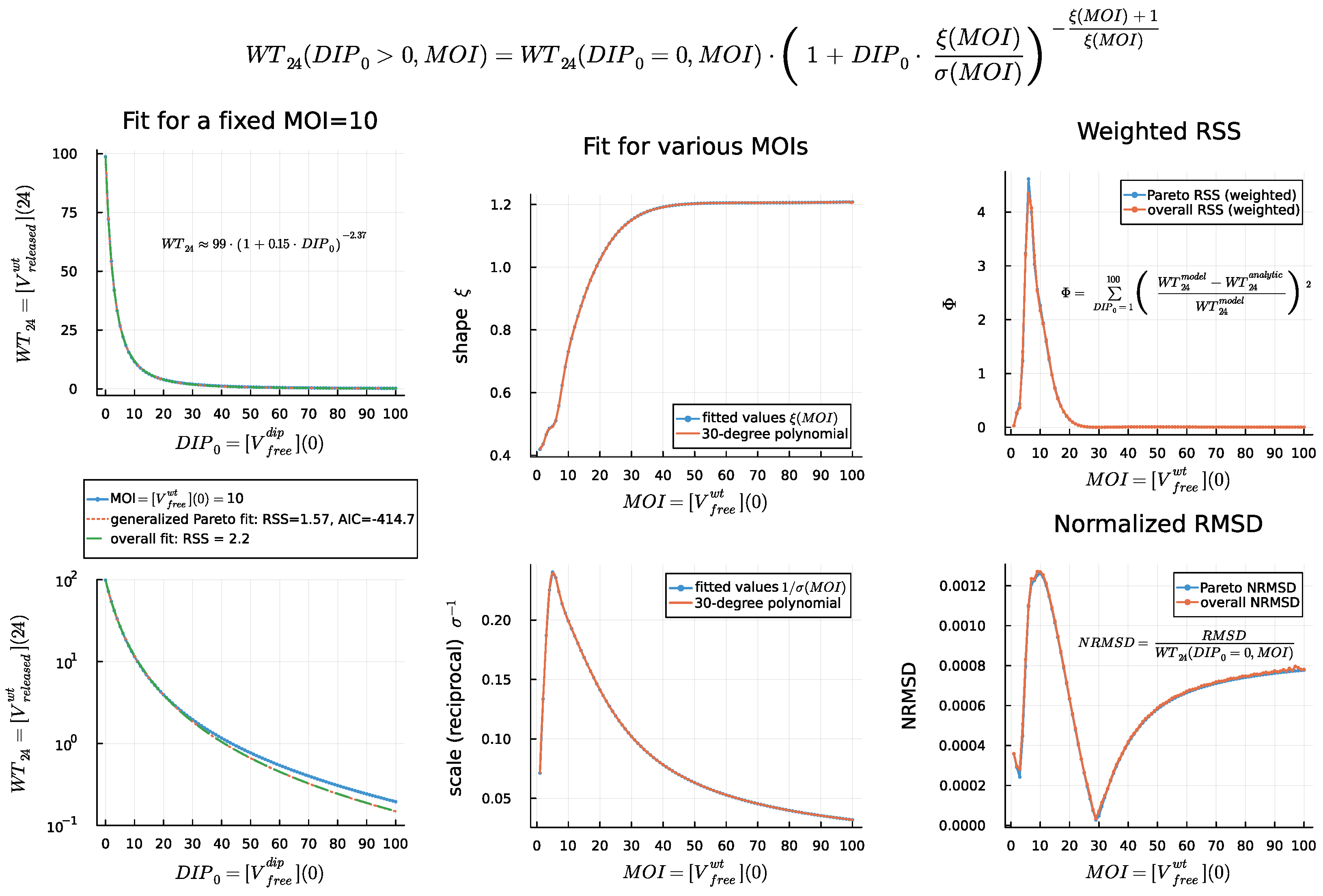
Given the predicted three-dimensional curves of model outputs as function of initial doses presented as heatmaps in Figure 8, we asked if the production of WT virions 24 h post-infection W T 24 = [ V r e l e a s e d w t ] ( 24 ) as function of initial doses M O I = [ V f r e e w t ] ( 0 ) and D I P 0 = [ V f r e e d i p ] ( 0 ) can be approximated by a compact analytic expression. Figure 9 shows that W T 24 as a function of D I P 0 , for a fixed M O I exhibits a decay that is slower than exponential (which would be displayed as a straight line on a logarithmic scale). Therefore, we used several analytical expressions with slower than exponential decay to fit the deterministic model predictions for WT virion production for fixed M O I = 10 . These include: (a) a Gompertz curve, and the probability density functions (p.d.f.) of (b) power-law, (c) Weibull, (d) Cauchy, (e) Burr, (f) Lomax, and (g) generalized Pareto heavy-tailed distributions. The error that was minimized is the sum of squares between the WT virion production, W T 24 , predicted by an analytic expression and predicted by the deterministic model for each D I P 0 ranging from 1 to 100. The generalized Pareto distribution (with a location parameter equal to zero) was chosen as the optimal analytic expression making use of the Akaike information criterion. The parameters of the generalized Pareto distribution ξ (shape) and σ (scale) can be fitted for different values of M O I , thus giving the functions ξ ( M O I ) and σ ( M O I ) . The overall parameterization is the following:
W T 24 ( D I P 0 > 0 , M O I ) W T 24 ( D I P 0 = 0 , M O I ) × 1 + D I P 0 · ξ ( M O I ) σ ( M O I ) ξ ( M O I ) + 1 ξ ( M O I ) ,
where W T 24 ( D I P 0 = 0 , M O I ) is the number of released WT virions 24 h post-infection with zero DIP initial dose for a given WT M O I .
Figure A4 shows the fit of a generalized Pareto function (28) for M O I = 10 and the dependence of parameters ξ and σ on M O I . One can see that the fit follows the data closely for suitable numbers of produced WT virions ( W T 24 > 1 ) and has some small discrepancies for W T 24 < 1 at large DIP doses D I P 0 > 40 . The dependences of parameters ξ ( M O I ) and 1 / σ ( M O I ) exhibit non-linear patterns. They can be approximated with a Hill function and a Dagum distribution p.d.f., respectively. However, when these analytic approximations are substituted in (28), the overall fit of (28) behaves approximately as an exponential decay function. Therefore, one should use the computed estimates of the parameters ξ and σ for every M O I , or approximate them with a higher degree polynomial that would follow the estimates closely, e.g., with a 30-degree Chebyshev polynomial as shown in Figure A4. Overall, the relative error of the fit (weighted residual sum of squares) of the closed-form expression (28) reaches its peak for M O I 6 , in the same region where the parameters ξ and σ shown a non-linear dependence on M O I . The root-mean-square deviation normalized to W T 24 ( D I P 0 = 0 , M O I ) , the maximum value of produced WT virions for each MOI, shows a similar increase near M O I 10 , as well as a later increase for large MOIs. This can be explained since the discrepancy in the tail of a generalized Pareto distribution corresponds to larger numbers of W T 24 with an increase of M O I . In summary, we have provided a closed-form expression, (28), as a prediction of the effect of DIPs on productive cell infection, i.e., the expected mean number of WT virions produced in a productive infection scenario for a range of relevant MOIs.

5. Discussion

SARS-CoV-2 still presents a real threat to human health as a result of several compounding factors: emergence of new strains due to mutation and waning immunity among vaccinated and unvaccinated individuals (for medical reasons or personal choice). Therefore, it is still important to investigate new treatment options, especially those that could be implemented early after infection, to alleviate pressure on healthcare systems. One such potential therapy is defective interfering particles. DIPs are virus-like particles with shorter genomes that require a wild-type (WT) virus to replicate. In this paper, we investigated the intra-cellular replication kinetics of WT virus in the presence of DIPs, making use of a mathematical model. To this end, we extended the model proposed by Grebennikov et al. in Ref. [21], which focused on the intra-cellular replication kinetics of SARS-CoV-2, to include co-infection with defective interfering particles, given their therapeutic potential [60,61]. In particular, we investigated the ability of DIPs to reduce WT viral load by competing for resources required to replicate or encapsulate the viral genome to form new virions. Since DIP genomes lack key fragments, they need a “helper” virus, which encodes non-structural and structural proteins, for their replication. There is evidence of DIPs leading to cause a reduction in viral titres for several viruses including: influenza A, dengue fever, and SARS-CoV-2 [14,15,62]. With the emergence of new SARS-CoV-2 strains, the effectiveness of a DIP particle (derived from a particular viral strain) against novel ones remains to be investigated.
Mathematical models of WT virus and DIP co-infection have been investigated at the within host-level and either consider a standard infection model with target, eclipse phase, and infected cells or include different localized areas of infection, such as the upper and lower respiratory tract [15,19]. There are, however, no models (to the best of our knowledge) that examine the intra-cellular replication kinetics of SARS-CoV-2 in the presence of DIPs. Our aim was to assess the hypothesis that DIPs lead to a reduction not only in the number of released WT virions, but also negatively impact the transcription of positive sense genomic RNAs. Additionally, we investigated the effects of initial infection dose (WT and DIP) in the release of both new WT virions and DIPs. Since experimental datasets are extremely limited, it is important to note that the parameter values obtained in this manuscript are based on the dataset used [15], and may not be globally identifiable. By globally identifiable we mean the identification of a unique parameter value from a dataset.
The extension of the model presented by Grebennikov et al. in Ref. [21] required new parameters to account for the kinetics of DIPs. Therefore, it was necessary to investigate the sensitivities of all model parameters. In particular, we made use of the Sobol sensitivity analysis to understand how variation in parameter values affects four different model outputs: [ g R N A w t ] , [ g R N A d i p ] , [ V r e l e a s e d w t ] , and [ V r e l e a s e d d i p ] . We found several parameters that have an effect on all four model outputs: K N S P , the threshold number of non-structural proteins, k t r ( ) w t / d i p , transcription rates of negative sense genomic RNA for WT virus and DIPs, respectively, and k t r ( + ) w t / d i p , the transcription rates for positive sense genomic RNA. The rates associated with cell entry, k f u s e and k u n c o a t , also lead to some variation in model outputs. Finally, if we examine as output WT and DIP release, we find their associated assembly rates, k a s s e m b l w t and k a s s e m b l d i p , as the most sensitive parameters.
DIPs have potential as therapeutics, and thus, it is important to explore how initial infection doses of WT and DIP alter the release of WT virus, to inform a treatment plan. We show that even a low MOI = 1 of DIPs can cause a reduction of approximately 50% in released WT virus compared to an infection in the absence of DIPs, with further reduction in released WT up to 10-fold for increasing MOI   w t and MOI   d i p . Figure 8 illustrates how increasing the dose of DIPs leads to a reduction in the fraction of released WT virions, in relation to the initial WT infection dose. These trends are consistent with the results from the stochastic model also developed in this paper (Figure A3). The doses of both WT virus and DIPs also had an effect on the probability of a productive infection, which decreased with increased doses of DIPs, but is almost certain for high doses of WT virus. We also investigated the effect of initial MOI of DIPs given a fixed dose of WT virus (MOI = 10) on viral particle release. Our results show that while DIP release peaks at an initial DIP dose of MOI = 5, the release of WT virions decreases in a dose-dependent manner. Furthermore, by an initial DIP dose of MOI = 40, WT virion release is effectively inhibited.
The deterministic and stochastic models we presented are a good first approximation to the kinetics of WT and DIP co-infection. Yet, there are a number of biological processes which have not been considered. First and foremost, we omitted the anti-viral response of the cell. While we need not consider the adaptive immune response since our time interval is 48 h, the innate immune response would play a pivotal role [63,64]. A family of cytosolic receptors, known as pattern recognition receptors (PRR), exists that detect viral RNAs to induce the production of type I interferons. Type I interferons (or viral IFNs), which are secreted by infected cells, include IFN- α , IFN- β , IFN- ω , and IFN- τ . These molecules are associated with activation of anti-viral cell states, which in turn lead to inhibition of viral replication and eventual viral clearance [65]. Furthermore, innate immune responses have been shown to be induced by DIP binding to PRRs, providing additional stimuli and magnifying the anti-viral cellular response [60]. As a consequence, it would, therefore, be ideal to extend the proposed model to consider the role of an innate immune response. Another limitation of our model is that for WT virions, we do not distinguish between infectious and non-infectious particles. This would be important to understand the potential infectivity of the viral particles released. We also fail to characterize the natural generation of DIPs during the WT replication cycle (which is inherently characterized by mutations). This process would contribute to the release of other defective interfering particles, and would potentially reduce the number of WT virions released. However, a complete calibration of such a model would require a dataset not currently at hand.
In our study, we have analyzed the possibility of utilizing the competitive interactions between viruses for the benefit of the infected host. Whether a similar phenomenon could be examined for other pathogens of major public concern, e.g., bacterial infections with Salmonella typhi Leptospira, using available mathematical models deserves a systematic multidisciplinary investigation [66,67].
Studies of other virus infections such as dengue virus, Zika virus, yellow fever virus respiratory syncytial virus, and influenza A virus showed that DIP treatment of human target cells inhibited virus production via activation of cellular innate immunity, which included interferon-dependent antiviral responses. Future direction of DIP-integrating mathematical modeling should incorporate a broad spectrum of virus–host interaction processes in order to robustly quantify and predict the function which the DIPs could have in vaccines, modulation of viral disease, innate immune responses, virus persistence, and virus evolution [68,69]. Although the DIPs offer a novel approach to antiviral therapy, the efforts to translate the in vitro studies to in vivo models are still limited. Recently, the Syrian hamster model of lethal Nipah virus (NiV) disease was used to examine the potential of DIPs to improve clinical outcomes. The results strongly support further research on the development and optimization of DIP-mediated treatment against high-consequence pathogens [70], which requires calibrated mathematical models as a powerful analytical tool.
To conclude, we believe the model we have proposed shows the potential benefits of DIPs as a therapeutic tool to reduce WT virus production. We also have shown that even low doses of these particles can have a positive effect on limiting WT virus production and reducing the probability of a successful infection. This reduction continues, in a dose-dependent manner, to greatly reduce WT virus production. Future work will focus on incorporating immune responses and the natural production of DIPs into the mathematical model presented here but will require further carefully curated data to assist in parameter estimation.

Author Contributions

Conceptualization, M.L. (Macauley Locke), D.G., M.L.-G., A.M., C.M.-P. and G.B.; methodology, M.L. (Macauley Locke), D.G., A.M., C.M.-P. and G.B.; software, M.L. (Macauley Locke) and D.G.; validation, M.L. (Macauley Locke), D.G., C.M.-P. and G.B.; formal analysis, M.L. (Macauley Locke), D.G. and I.S.; investigation, M.L. (Macauley Locke) and D.G.; resources, C.M.-P. and G.B.; data curation, A.M., M.L. (Marina Loguinova), C.M.-P. and G.B.; writing—original draft preparation, M.L. (Macauley Locke), D.G., C.M.-P. and G.B.; writing—review and editing, M.L. (Macauley Locke), D.G., I.S., M.L.-G., M.L. (Marina Loguinova), C.M.-P. and G.B.; visualization, M.L. (Macauley Locke), D.G. and I.S.; supervision, C.M.-P. and G.B.; project administration, C.M.-P. and G.B.; funding acquisition, D.G. and G.B. All authors have read and agreed to the published version of the manuscript.

Funding

G.B. and A.M. were supported by the Russian Science Foundation (research project number 23-11-00116). D.G. was financed by the Ministry of Science and Higher Education of the Russian Federation within the framework of state support for the creation and development of World-Class Research Centers “Digital biodesign and personalized healthcare” No. 075-15-2022-304. This manuscript has been internally reviewed at Los Alamos National Laboratory, and assigned the reference number LA-UR-22-29726 (CMP).

Data Availability Statement

The original data presented in the study are included in the article/appendix material, as well as made openly available in Github repository at https://github.com/MacauleyLockeml/SARS-CoV-2-DIP-Model (accessed on 12 June 2024).

Conflicts of Interest

The authors declare no conflicts of interest. The funders had no role in the design of the study; in the collection, analyses, or interpretation of data; in the writing of the manuscript; or in the decision to publish the results.

Abbreviations

The following abbreviations are used in this manuscript:
ABCApproximate Bayesian computation
MCMarkov chain
MOIMultiplicity of infection
ODEOrdinary differential equation
SDEStochastic differential equation
RSSARejection stochastic simulation algorithm
TIPTherapeutic interfering particle
DIP    Defective interfering particle
WTWild-type

Appendix A

Figure A1. Posterior histograms. Posterior histograms of the top 0.1 % sampled parameter sets from a total of 10 6 accepted sets. Table 4 lists the search ranges used to obtain the above posterior histograms. Purple histogram: posterior histogram of accepted parameter sets; blue histogram: histogram of prior beliefs; and black dashed line: the median parameter value listed in Table 4 used to generate Figure 4, Figure 5, Figure 6, Figure 7, Figure 8 and Figure 9.
Mathematics 12 01904 g0a1
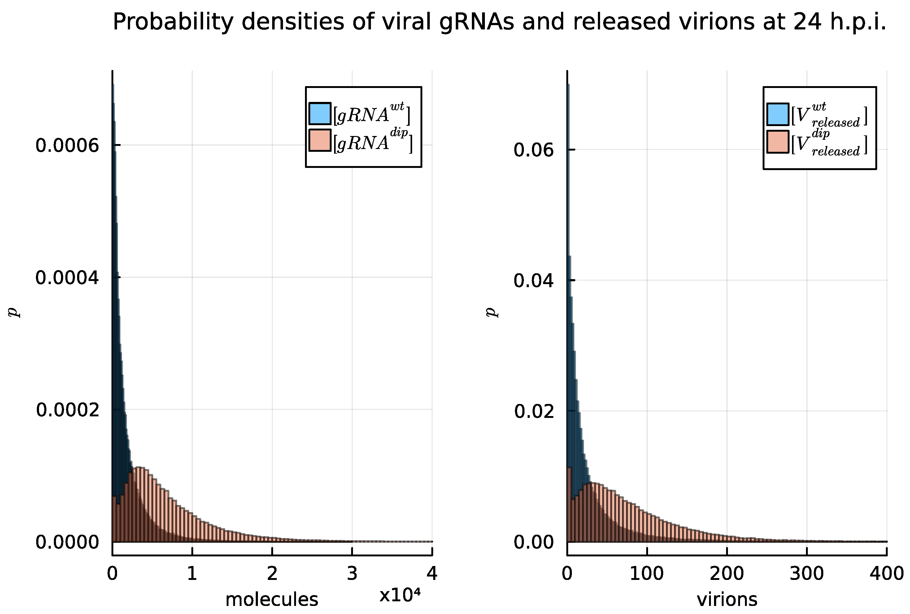
Figure A2. Stochastic model outputs 24 h post-infection. The histograms for the numbers of (left) genomic RNA ( [ g R N A w t ] ( 24 ) , [ g R N A d i p ] ( 24 ) ) and (right) produced virions ( [ V r e l e a s e d w t ] ( 24 ) , [ V r e l e a s e d d i p ] ( 24 ) ) are shown for an ensemble of 10 6 stochastic simulations with initial doses [ V f r e e w t ] ( 0 ) = 10 and [ V f r e e d i p ] ( 0 ) = 10 . The histograms are normalized to approximate a true probability density distribution.
Mathematics 12 01904 g0a2
Figure A3. Effects of varying initial dose on viral particle release (as predicted by the stochastic model). (left panels): Median values, (right panels): mean values are presented as the outputs of ensembles of 10 5 trajectories simulated for each combination of the initial conditions. (top): Total WT virions released over the 24 h post-infection for varying initial conditions of free WT virions [ V f r e e w t ] ( 0 ) = 0 –20 and free DIPs [ V f r e e d i p ] ( 0 ) = 0 –20 from the stochastic model. (bottom): Total DIP particles released for varying initial doses. The isolines shown on the heatmaps as white lines coincide with the corresponding ticks in the colorbars.
Mathematics 12 01904 g0a3
Figure A4. Fitting WT virion production as a function of initial DIP doses with analytic expression. (left): fit of the deterministic model output (blue lines) for fixed M O I = 10 using Equation (28), which is based on the probability density function of a generalized Pareto distribution (red dotted and green dashed lines). The upper plot is presented in linear scale, the lower one in logarithmic scale. The formula with estimated parameters is shown in the annotation of the upper plot. (center): fit of the parameters of the analytic expression (28) for various MOIs. The upper plot shows the fitted values of the parameter ξ and the lower one the reciprocal of the parameter σ . The fitted estimates ξ ( M O I ) and 1 / σ ( M O I ) can be approximated closely with a 30-degree Chebyshev polynomial (red lines). The overall fit in the left panel denotes the fit with Equation (28), where the polynomials are used as ξ ( M O I ) and 1 / σ ( M O I ) . (right): the error of the fit with Equation (28) for various MOIs. The upper plot shows the residual sum of squares (RSS) weighted by the data values for each D I P 0 . The lower plot shows the root-mean-square deviation (RMSD) normalized by the number of produced WT virions with D I P 0 = 0 .
Mathematics 12 01904 g0a4
Figure A5. The estimation of the effect of DIP dose, D I P 0 , on the probability of productive infection as a function of MOI. (left): for each MOI, the probability decreases linearly as D I P 0 increases. (right): the linear decay rate, β w t , and therefore, the effect of D I P 0 decreases with an increase in MOI.
Mathematics 12 01904 g0a5

References

  1. Wu, D.; Wu, T.; Liu, Q.; Yang, Z. The SARS-CoV-2 outbreak: What we know. Int. J. Infect. Dis. 2020, 94, 44–48. [Google Scholar] [CrossRef]
  2. Li, X.; Wang, W.; Zhao, X.; Zai, J.; Zhao, Q.; Li, Y.; Chaillon, A. Transmission dynamics and evolutionary history of 2019-nCoV. J. Med. Virol. 2020, 92, 501–511. [Google Scholar] [CrossRef]
  3. Martellucci, C.A.; Flacco, M.E.; Cappadona, R.; Bravi, F.; Mantovani, L.; Manzoli, L. SARS-CoV-2 pandemic: An overview. Adv. Biol. Regul. 2020, 77, 100736. [Google Scholar] [CrossRef]
  4. World Health Organization. Coronavirus Disease 2019 (COVID-19): Situation Report, 73; World Health Organization: Geneva, Switzerland, 2020.
  5. Colson, P.; Rolain, J.M.; Raoult, D. Chloroquine for the 2019 novel coronavirus SARS-CoV-2, 2020. Int. J. Antimicrob. Agents 2020, 55, 105923. [Google Scholar] [CrossRef]
  6. Morse, J.S.; Lalonde, T.; Xu, S.; Liu, W.R. Learning from the past: Possible urgent prevention and treatment options for severe acute respiratory infections caused by 2019-nCoV. Chembiochem 2020, 21, 730–738. [Google Scholar] [CrossRef]
  7. Castells, M.C.; Phillips, E.J. Maintaining safety with SARS-CoV-2 vaccines. N. Engl. J. Med. 2021, 384, 643–649. [Google Scholar] [CrossRef]
  8. Boehm, E.; Kronig, I.; Neher, R.A.; Eckerle, I.; Vetter, P.; Kaiser, L. Novel SARS-CoV-2 variants: The pandemics within the pandemic. Clin. Microbiol. Infect. 2021, 27, 1109–1117. [Google Scholar] [CrossRef]
  9. Jangra, S.; Ye, C.; Rathnasinghe, R.; Stadlbauer, D.; Alshammary, H.; Amoako, A.A.; Awawda, M.H.; Beach, K.F.; Bermúdez-González, M.C.; Chernet, R.L.; et al. SARS-CoV-2 spike E484K mutation reduces antibody neutralisation. Lancet Microbe 2021, 2, e283–e284. [Google Scholar] [CrossRef]
  10. Naqvi, A.A.T.; Fatima, K.; Mohammad, T.; Fatima, U.; Singh, I.K.; Singh, A.; Atif, S.M.; Hariprasad, G.; Hasan, G.M.; Hassan, M.I. Insights into SARS-CoV-2 genome, structure, evolution, pathogenesis and therapies: Structural genomics approach. Biochim. Biophys. Acta Mol. Basis Dis. 2020, 1866, 165878. [Google Scholar] [CrossRef]
  11. Fu, Y.; Cheng, Y.; Wu, Y. Understanding SARS-CoV-2-mediated inflammatory responses: From mechanisms to potential therapeutic tools. Virol. Sin. 2020, 35, 266–271. [Google Scholar] [CrossRef]
  12. Alnaji, F.G.; Brooke, C.B. Influenza virus DI particles: Defective interfering or delightfully interesting? PloS Pathog. 2020, 16, e1008436. [Google Scholar] [CrossRef]
  13. Fatehi, F.; Bingham, R.J.; Dechant, P.P.; Stockley, P.G.; Twarock, R. Therapeutic interfering particles exploiting viral replication and assembly mechanisms show promising performance: A modelling study. Sci. Rep. 2021, 11, 23847. [Google Scholar] [CrossRef]
  14. Bdeir, N.; Arora, P.; Gärtner, S.; Hoffmann, M.; Reichl, U.; Pöhlmann, S.; Winkler, M. A system for production of defective interfering particles in the absence of infectious influenza A virus. PLoS ONE 2019, 14, e0212757. [Google Scholar] [CrossRef]
  15. Chaturvedi, S.; Vasen, G.; Pablo, M.; Chen, X.; Beutler, N.; Kumar, A.; Tanner, E.; Illouz, S.; Rahgoshay, D.; Burnett, J.; et al. Identification of a therapeutic interfering particle—A single-dose SARS-CoV-2 antiviral intervention with a high barrier to resistance. Cell 2021, 184, 6022–6036. [Google Scholar] [CrossRef]
  16. Smither, S.J.; Garcia-Dorival, I.; Eastaugh, L.; Findlay, J.S.; O’Brien, L.M.; Carruthers, J.; Williamson, E.D.; Molina-París, C.; Hiscox, J.A.; Laws, T.R. An Investigation of the Effect of Transfected Defective, Ebola Virus Genomes on Ebola Replication. Front. Cell. Infect. Microbiol. 2020, 10, 159. [Google Scholar] [CrossRef]
  17. Rouzine, I.M.; Weinberger, L.S. Design requirements for interfering particles to maintain coadaptive stability with HIV-1. J. Virol. 2013, 87, 2081–2093. [Google Scholar] [CrossRef]
  18. Grebennikov, D.; Karsonova, A.; Loguinova, M.; Casella, V.; Meyerhans, A.; Bocharov, G. Predicting the Kinetic Coordination of Immune Response Dynamics in SARS-CoV-2 Infection: Implications for Disease Pathogenesis. Mathematics 2022, 10, 3154. [Google Scholar] [CrossRef]
  19. Perelson, A.S.; Ke, R. Mechanistic modeling of SARS-CoV-2 and other infectious diseases and the effects of therapeutics. Clin. Pharmacol. Ther. 2021, 109, 829–840. [Google Scholar] [CrossRef]
  20. Zhao, Y.; Xing, Y. A delayed dynamical model for COVID-19 therapy with defective interfering particles and artificial antibodies. Discret. Contin. Dyn.-Syst.-B 2021, 27, 5367. [Google Scholar] [CrossRef]
  21. Grebennikov, D.; Kholodareva, E.; Sazonov, I.; Karsonova, A.; Meyerhans, A.; Bocharov, G. Intracellular Life Cycle Kinetics of SARS-CoV-2 Predicted Using Mathematical Modelling. Viruses 2021, 13, 1735. [Google Scholar] [CrossRef]
  22. Zhang, X.Y.; Trame, M.N.; Lesko L, J.; Schmidt, S. Sobol Sensitivity Analysis: A Tool to Guide the Development and Evaluation of Systems Pharmacology Models. Pharmacometrics Syst. Pharmacol. 2015, 4, 69–79. [Google Scholar] [CrossRef]
  23. Saltelli, A.; Ratto, M.; Andres, T.; Campolongo, F.; Cariboni, J.; Gatelli, D.; Saisana, M.; Tarantola, S. Global Sensitivity Analysis. The Primer, 1st ed.; Wiley: Hoboken, NJ, USA, 2007. [Google Scholar]
  24. Sobol, I.M. Sensitivity analysis for non-linear mathematical models. Math. Model. Comput. Exp. 1993, 1, 407–414. [Google Scholar]
  25. Saltelli, A.; Tarantola, S.; Campolongo, F.; Ratto, M. Sensitivity Analysis in Practice: A Guide to Assessing Scientific Models; Wiley: Hoboken, NJ, USA, 2004. [Google Scholar]
  26. Ozono, S.; Zhang, Y.; Ode, H.; Sano, K.; Tan, T.S.; Imai, K.; Miyoshi, K.; Kishigami, S.; Ueno, T.; Iwatani, Y.; et al. SARS-CoV-2 D614G spike mutation increases entry efficiency with enhanced ACE2-binding affinity. Nat. Commun. 2021, 12, 848. [Google Scholar] [CrossRef]
  27. Walls, A.C.; Park, Y.J.; Tortorici, M.A.; Wall, A.; McGuire, A.T.; Veesler, D. Structure, function, and antigenicity of the SARS-CoV-2 spike glycoprotein. Cell 2020, 181, 281–292. [Google Scholar] [CrossRef]
  28. Baggen, J.; Persoons, L.; Vanstreels, E.; Jansen, S.; Van Looveren, D.; Boeckx, B.; Geudens, V.; De Man, J.; Jochmans, D.; Wauters, J.; et al. Genome-wide CRISPR screening identifies TMEM106B as a proviral host factor for SARS-CoV-2. Nat. Genet. 2021, 53, 435–444. [Google Scholar] [CrossRef]
  29. Bocharov, G.; Romanyukha, A. Mathematical model of antiviral immune response III. Influenza A virus infection. J. Theor. Biol. 1994, 167, 323–360. [Google Scholar] [CrossRef]
  30. Baccam, P.; Beauchemin, C.; Macken, C.A.; Hayden, F.G.; Perelson, A.S. Kinetics of influenza A virus infection in humans. J. Virol. 2006, 80, 7590–7599. [Google Scholar] [CrossRef]
  31. Zhu, Y.; Yu, D.; Yan, H.; Chong, H.; He, Y. Design of potent membrane fusion inhibitors against SARS-CoV-2, an emerging coronavirus with high fusogenic activity. J. Virol. 2020, 94, e00635-20. [Google Scholar] [CrossRef]
  32. Heldt, F.S.; Kupke, S.Y.; Dorl, S.; Reichl, U.; Frensing, T. Single-cell analysis and stochastic modelling unveil large cell-to-cell variability in influenza A virus infection. Nat. Commun. 2015, 6, 8938. [Google Scholar] [CrossRef]
  33. Irigoyen, N.; Firth, A.E.; Jones, J.D.; Chung, B.Y.W.; Siddell, S.G.; Brierley, I. High-resolution analysis of coronavirus gene expression by RNA sequencing and ribosome profiling. PLoS Pathog. 2016, 12, e1005473. [Google Scholar] [CrossRef]
  34. Buccitelli, C.; Selbach, M. mRNAs, proteins and the emerging principles of gene expression control. Nat. Rev. Genet. 2020, 21, 630–644. [Google Scholar] [CrossRef]
  35. Kim, D.; Lee, J.Y.; Yang, J.S.; Kim, J.W.; Kim, V.N.; Chang, H. The architecture of SARS-CoV-2 transcriptome. Cell 2020, 181, 914–921. [Google Scholar] [CrossRef]
  36. Gasteiger, E.; Gattiker, A.; Hoogland, C.; Ivanyi, I.; Appel, R.D.; Bairoch, A. ExPASy: The proteomics server for in-depth protein knowledge and analysis. Nucleic Acids Res. 2003, 31, 3784–3788. [Google Scholar] [CrossRef]
  37. Nelson, D.L.; Lehninger, A.L.; Cox, M.M. Lehninger Principles of Biochemistry; Macmillan: New York, NY, USA, 2008. [Google Scholar]
  38. Adelman, K.; La Porta, A.; Santangelo, T.J.; Lis, J.T.; Roberts, J.W.; Wang, M.D. Single molecule analysis of RNA polymerase elongation reveals uniform kinetic behavior. Proc. Natl. Acad. Sci. USA 2002, 99, 13538–13543. [Google Scholar] [CrossRef]
  39. Klein, S.; Cortese, M.; Winter, S.L.; Wachsmuth-Melm, M.; Neufeldt, C.J.; Cerikan, B.; Stanifer, M.L.; Boulant, S.; Bartenschlager, R.; Chlanda, P. SARS-CoV-2 structure and replication characterized by in situ cryo-electron tomography. Nat. Commun. 2020, 11, 5885. [Google Scholar] [CrossRef]
  40. Zinzula, L.; Basquin, J.; Bohn, S.; Beck, F.; Klumpe, S.; Pfeifer, G.; Nagy, I.; Bracher, A.; Hartl, F.U.; Baumeister, W. High-resolution structure and biophysical characterization of the nucleocapsid phosphoprotein dimerization domain from the COVID-19 severe acute respiratory syndrome coronavirus 2. Biochem. Biophys. Res. Commun. 2021, 538, 54–62. [Google Scholar] [CrossRef]
  41. Chen, I.J.; Yuann, J.M.P.; Chang, Y.M.; Lin, S.Y.; Zhao, J.; Perlman, S.; Shen, Y.Y.; Huang, T.H.; Hou, M.H. Crystal structure-based exploration of the important role of Arg106 in the RNA-binding domain of human coronavirus OC43 nucleocapsid protein. Biochim. Biophys. Acta Proteins Proteom. 2013, 1834, 1054–1062. [Google Scholar] [CrossRef]
  42. Spencer, K.A.; Hiscox, J.A. Characterisation of the RNA binding properties of the coronavirus infectious bronchitis virus nucleocapsid protein amino-terminal region. FEBS Lett. 2006, 580, 5993–5998. [Google Scholar] [CrossRef]
  43. Spencer, K.A.; Dee, M.; Britton, P.; Hiscox, J.A. Role of phosphorylation clusters in the biology of the coronavirus infectious bronchitis virus nucleocapsid protein. Virology 2008, 370, 373–381. [Google Scholar] [CrossRef]
  44. Bar-On, Y.M.; Flamholz, A.; Phillips, R.; Milo, R. Science Forum: SARS-CoV-2 (COVID-19) by the numbers. elife 2020, 9, e57309. [Google Scholar] [CrossRef]
  45. Jack, A.; Ferro, L.S.; Trnka, M.J.; Wehri, E.; Nadgir, A.; Nguyenla, X.; Fox, D.; Costa, K.; Stanley, S.; Schaletzky, J.; et al. SARS-CoV-2 nucleocapsid protein forms condensates with viral genomic RNA. PLoS Biol. 2021, 19, e3001425. [Google Scholar] [CrossRef]
  46. Cubuk, J.; Alston, J.J.; Incicco, J.J.; Singh, S.; Stuchell-Brereton, M.D.; Ward, M.D.; Zimmerman, M.I.; Vithani, N.; Griffith, D.; Wagoner, J.A.; et al. The SARS-CoV-2 nucleocapsid protein is dynamic, disordered, and phase separates with RNA. Nat. Commun. 2021, 12, 1–17. [Google Scholar] [CrossRef]
  47. Viehweger, A.; Krautwurst, S.; Lamkiewicz, K.; Madhugiri, R.; Ziebuhr, J.; Hölzer, M.; Marz, M. Direct RNA nanopore sequencing of full-length coronavirus genomes provides novel insights into structural variants and enables modification analysis. Genome Res. 2019, 29, 1545–1554. [Google Scholar] [CrossRef]
  48. Neuman, B.W.; Kiss, G.; Kunding, A.H.; Bhella, D.; Baksh, M.F.; Connelly, S.; Droese, B.; Klaus, J.P.; Makino, S.; Sawicki, S.G.; et al. A structural analysis of M protein in coronavirus assembly and morphology. J. Struct. Biol. 2011, 174, 11–22. [Google Scholar] [CrossRef]
  49. Yao, H.; Song, Y.; Chen, Y.; Wu, N.; Xu, J.; Sun, C.; Zhang, J.; Weng, T.; Zhang, Z.; Wu, Z.; et al. Molecular architecture of the SARS-CoV-2 virus. Cell 2020, 183, 730–738. [Google Scholar] [CrossRef]
  50. Gordon, D.E.; Hiatt, J.; Bouhaddou, M.; Rezelj, V.V.; Ulferts, S.; Braberg, H.; Jureka, A.S.; Obernier, K.; Guo, J.Z.; Batra, J.; et al. Comparative host-coronavirus protein interaction networks reveal pan-viral disease mechanisms. Science 2020, 370, eabe9403. [Google Scholar] [CrossRef]
  51. Shcherbatova, O.; Grebennikov, D.; Sazonov, I.; Meyerhans, A.; Bocharov, G. Modeling of the HIV-1 life cycle in productively infected cells to predict novel therapeutic targets. Pathogens 2020, 9, 255. [Google Scholar] [CrossRef]
  52. Mooney, J.; Thakur, S.; Kahng, P.; Trapani, J.G.; Poccia, D. Quantification of exocytosis kinetics by DIC image analysis of cortical lawns. J. Chem. Biol. 2014, 7, 43–55. [Google Scholar] [CrossRef]
  53. Toni, T.; Welch, D.; Strelkowa, N.; Ipsen, A.; Stumpf, M.P. Approximate Bayesian computation scheme for parameter inference and model selection in dynamical systems. J. R. Soc. Interface 2009, 6, 187–202. [Google Scholar] [CrossRef]
  54. Gillespie, D.T. Stochastic Simulation of Chemical Kinetics. Annu. Rev. Phys. Chem. 2007, 58, 35–55. [Google Scholar] [CrossRef]
  55. Marchetti, L.; Priami, C.; Thanh, V.H. Simulation Algorithms for Computational Systems Biology; Texts in Theoretical Computer Science; An EATCS Series; Springer International Publishing: Cham, Switzerland, 2017. [Google Scholar]
  56. Sazonov, I.; Grebennikov, D.; Meyerhans, A.; Bocharov, G. Markov Chain-Based Stochastic Modelling of HIV-1 Life Cycle in a CD4 T Cell. Mathematics 2021, 9, 2025. [Google Scholar] [CrossRef]
  57. V’kovski, P.; Kratzel, A.; Steiner, S.; Stalder, H.; Thiel, V. Coronavirus biology and replication: Implications for SARS-CoV-2. Nat. Rev. Microbiol. 2021, 19, 155–170. [Google Scholar] [CrossRef]
  58. Mendonça, L.; Howe, A.; Gilchrist, J.B.; Sheng, Y.; Sun, D.; Knight, M.L.; Zanetti-Domingues, L.C.; Bateman, B.; Krebs, A.S.; Chen, L.; et al. Correlative multi-scale cryo-imaging unveils SARS-CoV-2 assembly and egress. Nat. Commun. 2021, 12, 4629. [Google Scholar] [CrossRef]
  59. Sazonov, I.; Grebennikov, D.; Meyerhans, A.; Bocharov, G. Sensitivity of SARS-CoV-2 Life Cycle to IFN Effects and ACE2 Binding Unveiled with a Stochastic Model. Viruses 2022, 14, 403. [Google Scholar] [CrossRef]
  60. Rand, U.; Kupke, S.Y.; Shkarlet, H.; Hein, M.D.; Hirsch, T.; Marichal-Gallardo, P.; Cicin-Sain, L.; Reichl, U.; Bruder, D. Antiviral activity of influenza A virus defective interfering particles against SARS-CoV-2 replication in vitro through stimulation of innate immunity. Cells 2021, 10, 1756. [Google Scholar] [CrossRef]
  61. Roux, L.; Simon, A.E.; Holland, J.J. Effects of defective interfering viruses on virus replication and pathogenesis in vitro and in vivo. Adv. Virus Res. 1991, 40, 181–211. [Google Scholar]
  62. Li, D.; Lin, M.H.; Rawle, D.J.; Jin, H.; Wu, Z.; Wang, L.; Lor, M.; Hussain, M.; Aaskov, J.; Harrich, D. Dengue virus-free defective interfering particles have potent and broad anti-dengue virus activity. Commun. Biol. 2021, 4, 557. [Google Scholar] [CrossRef]
  63. Dempsey, P.; Vaidya, S.; Cheng, G. The art of war: Innate and adaptive immune responses. Cell. Mol. Life Sci. 2003, 60, 2604–2621. [Google Scholar] [CrossRef]
  64. tenOever, B. The Evolution of Antiviral Defense Systems. Cell Host Microbe 2016, 19, 142–149. [Google Scholar] [CrossRef]
  65. Katze, M.G.; He, Y.; Gale, M. Viruses and interferon: A fight for supremacy. Nat. Rev. Immunol. 2002, 2, 675–687. [Google Scholar]
  66. Alalhareth, F.K.; Atta, U.; Ali, A.H.; Ahmad, A.; Alharbi, M.H. Analysis of Leptospirosis transmission dynamics with environmental effects and bifurcation using fractional-order derivative. Alex. Eng. J. 2023, 80, 372–382. [Google Scholar] [CrossRef]
  67. Dayan, F.; Ahmed, N.; Ali, A.H.; Rafiq, M.; Raz, A. Numerical investigation of a typhoid disease model in fuzzy environment. Sci. Rep. 2023, 13, 21993. [Google Scholar] [CrossRef]
  68. Lin, M.H.; Li, D.; Tang, B.; Li, L.; Suhrbier, A.; Harrich, D. Defective Interfering Particles with Broad-Acting Antiviral Activity for Dengue, Zika, Yellow Fever, Respiratory Syncytial and SARS-CoV-2 Virus Infection. Microbiol. Spectr. 2022, 10, e03949-22. [Google Scholar] [CrossRef]
  69. Wu, M.; Zhou, E.; Sheng, R.; Fu, X.; Li, J.; Jiang, C.; Su, W. Defective Interfering Particles of Influenza Virus and Their Characteristics, Impacts, and Use in Vaccines and Antiviral Strategies: A Systematic Review. Viruses 2022, 14, 2773. [Google Scholar] [CrossRef]
  70. Welch, S.R.; Spengler, J.R.; Harmon, J.R.; Coleman-McCray, J.D.; Scholte, F.E.M.; Genzer, S.C.; Lo, M.K.; Montgomery, J.M.; Nichol, S.T.; Spiropoulou, C.F. Defective Interfering Viral Particle Treatment Reduces Clinical Signs and Protects Hamsters from Lethal Nipah Virus Disease. mBio 2022, 13, e03294-21. [Google Scholar] [CrossRef]
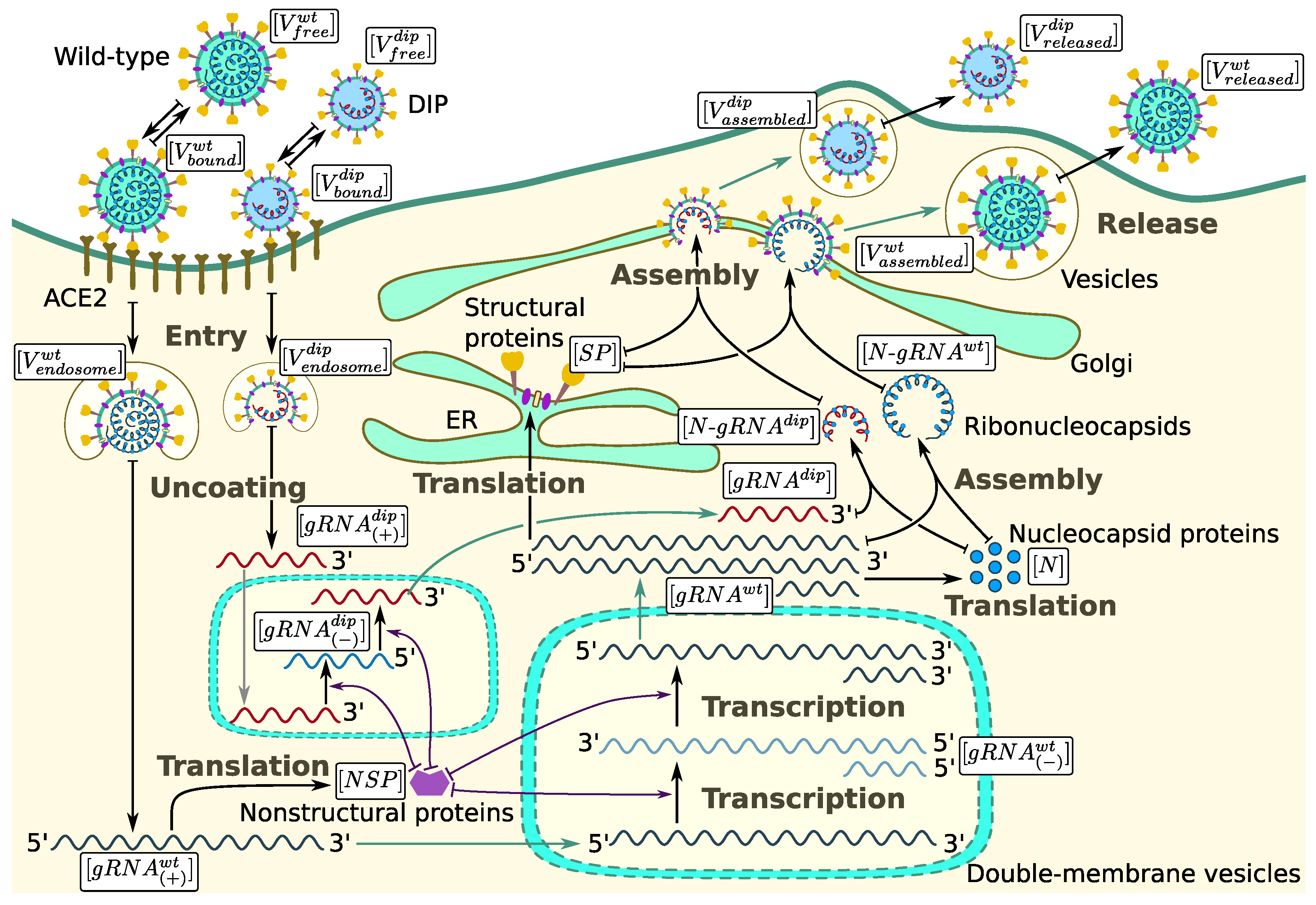
Figure 1. Biological scheme of the replication of infectious SARS-CoV-2 and defective interfering viral particles. Arrows without a T-end (which are not green) indicate the synthesis processes, i.e., translation or transcription, arrows with T-shaped beginning indicate that the variable at which the arrow points with the arrow-end is increased, while the variable at which the arrow points with a T-end is decreased (e.g., transitions of the entities from one state to another, or a decrease of non-structural proteins during the transcription activation), and green arrows indicate the transport of the entities from one place to another (to or from double-membrane vesicles or to the cell membrane in vesicles), which is not modeled explicitly. All entities are subject to degradation.
Mathematics 12 01904 g001
Figure 2. Sensitivity results for genomic RNA. First- and total-order Sobol’ sensitivity indices from 10 4 samples with 95% confidence interval (black line). (left): sensitivities for [ g R N A d i p ] ( 48 ) . (right): sensitivities for [ g R N A w t ] ( 48 ) . Initial conditions were [ V f r e e w t ] ( 0 ) = 10 and [ V f r e e d i p ] ( 0 ) = 10 .
Mathematics 12 01904 g002
Figure 3. Sensitivity results for released particles. First- and total-order Sobol’ sensitivity indices from 10 4 samples with 95% confidence interval (black line). (left): sensitivities for [ V r e l e a s e d d i p ] ( 48 ) . (right): sensitivities for [ V r e l e a s e d w t ] ( 48 ) . Initial conditions of [ V f r e e w t ] ( 0 ) = 10 and [ V f r e e d i p ] ( 0 ) = 10 were used.
Mathematics 12 01904 g003
Figure 4. Dynamics of viral particle production. Viral particle release kinetics predicted by the model for the parameter values from Table 4 with initial conditions [ V f r e e w t ] ( 0 ) = 10 and [ V f r e e d i p ] ( 0 ) = 10 during 48 h post-infection. The calibration was performed using ABC method and data from Chaturvedi et al. [15]. (Yellow line): the reference solution to a model where DIPs are not considered in the replication dynamics. (Red line): the production of WT virions [ V r e l e a s e d w t ] with DIPs (blue line): [ V r e l e a s e d d i p ] .
Mathematics 12 01904 g004
Figure 5. Deterministic model outputs. Dynamics of the model state variables with initial conditions [ V f r e e w t ] ( 0 ) = 10 and [ V f r e e d i p ] ( 0 ) = 10 over a 48 h time course. (upper left): free WT or DIP virions bind and fuse to the cell and (upper right): virions entering endosomes and uncoating of viral positive sense genomic RNA. (middle left): generation of a negative sense genome and ORF1 to form non-structural proteins ( N S P s) and (middle right): the production of positive sense genomic RNAs and N protein. (bottom left): translation of structural proteins and formation of ribonucleocapsid molecules and (bottom right): assembly and release of WT virions and DIPs. Dashed lines represent the reference model solution from Ref. [21].
Mathematics 12 01904 g005aMathematics 12 01904 g005b
Figure 6. Stochastic model outputs. Statistics of the stochastic model trajectories with initial conditions [ V f r e e w t ] ( 0 ) = 10 and [ V f r e e d i p ] ( 0 ) = 10 over a 24 h time course for an ensemble of 10 6 realization. Solid lines: medians, dashed lines: mean values, filled areas: inter-quartile ranges.
Mathematics 12 01904 g006
Figure 7. Probability of productive infection for varying initial doses of both WT [ V f r e e w t ] ( 0 ) = 1 –20 and DIPs [ V f r e e d i p ] ( 0 ) = 1 –20 at 24 h post-infection. (left): dependence on [ V f r e e w t ] ( 0 ) for various [ V f r e e d i p ] ( 0 ) , (right): dependence on [ V f r e e d i p ] ( 0 ) for various [ V f r e e w t ] ( 0 ) .
Mathematics 12 01904 g007
Figure 8. Effects of initial doses on viral production. (top): total WT virions and (bottom): DIP particles released over the 24 h post-infection for varying initial numbers of WT virions [ V f r e e w t ] ( 0 ) = 0 –20 and DIPs [ V f r e e d i p ] ( 0 ) = 0 –20 predicted by the deterministic model. The isolines (white lines) correspond to the white ticks in the colorbars.
Mathematics 12 01904 g008
Figure 9. Effect of initial dose of DIPs on virion production. Total viral particle released kinetics for initial values of [ V f r e e w t ] ( 0 ) ranging from 3 to 20 virions, as a function of DIP doses [ V f r e e d i p ] ( 0 ) = 1 –100.
Mathematics 12 01904 g009
Table 1. Dynamical variables of the mathematical model for the life cycle of SARS-CoV-2, with defective interfering particles.
Variable DefinitionValue
[ V f r e e w t ] Number of free infectious (i.e., wild-type) virions outside the cell membrane10
[ V b o u n d w t ] Number of infectious virions bound to ACE2 and activated by TMPRSS21–10
[ V e n d o s o m e w t ] Number of infectious virions in endosomes1–10
[ V f r e e d i p ] Number of free non-infectious (i.e., defective interfering particles) virions
outside the cell membrane
[ V b o u n d d i p ] Number of non-infectious virions bound to ACE2 and activated by TMPRSS2
[ V e n d o s o m e d i p ] Number of non-infectious virions in endosomes
[ g R N A ( + ) w t ] Single strand positive sense genomic RNA1–5
[ g R N A ( + ) d i p ] Single strand positive sense DIP genomic RNA
[ N S P ] Population of non-structural proteins
[ g R N A ( ) w t ] Negative sense genomic and subgenomic RNAs of infectious virus10
[ g R N A w t ] Positive sense genomic and subgenomic RNAs of infectious virus 10 4
[ g R N A ( ) d i p ] Negative sense subgenomic RNAs of DIPs
[ g R N A d i p ] Positive sense subgenomic RNAs of DIPs
[ S P ] Total number of structural proteins S + M + E per virion 2 × 10 3 ( 1 , 125 , 2230 )
[ N ] N proteins per virion456; 1465 ( 730 , 2200 )
[ N - g R N A w t ] Ribonucleocapsid molecules for infectious virions
[ N - g R N A d i p ] Ribonucleocapsid molecules for non-infectious virions
[ V a s s e m b l e d w t ] Assembled infectious virions in endosomes
[ V r e l e a s e d w t ] Released infectious viruses10– 10 4 virions
in 7 to 24 h
[ V a s s e m b l e d d i p ] Assembled non-infectious virions in endosomes
[ V r e l e a s e d d i p ] Released non-infectious virions
Table 2. Estimates of previously calibrated model parameter values.
ParameterDescription, UnitsValueRange [References]
k b i n d Rate of virion binding to ACE2 receptor, h   1 12(3.6, 12) [26,27]
d V w t Clearance rate of WT extracellular virions, h   1 0.12(0.06, 3.5) [28,29,30]
k d i s s Dissociation rate constant of bound virions, h   1 0.61(0.32, 1.08) [26,27]
k f u s e Fusion rate constant, h   1 0.5(0.33, 1) [31]
k u n c o a t Uncoating rate constant, h   1 0.5(0.33, 1) [31]
d e n d o s o m e w t Degradation rate of WT virions in endosomes, h   1 0.06(0.0001, 0.12) [28,32],
k t r a n s l Translation rate, nt/mRNA h   1 45,360(40,000, 50,000) [33,34]
1 / f O R F 1 Length of ORF1 of the RNA genome coding N S P s, nt21,000fixed [35]
d N S P Degradation rate of proteins in the cell, h   1 0.069(0.023, 0.69) [34,36],
tuned to (0.023, 0.1)
k t r ( ) w t Transcription rate of WT negative sense3(1, 100) [34],
Genomic and subgenomic RNAs, copies/mRNA h   1 tuned to (1, 20)
K N S P Threshold number of N S P s100(10, 150)
enhancing vRNA transcription, molecules
d g R N A w t Degradation rate of WT positive sense RNAs in cell, h   1 0.2(0.069, 0.69) [34,37],
tuned to (0.069, 0.4)
d g R N A ( ) w t Degradation rate of WT negative sense RNAs0.1(0.05, 0.2)
in double-membrane vesicles, h   1
k t r ( + ) w t Replication rate of positive sense WT RNAs, copies/mRNA/h1000(620, 1380) [38]
k c o m p l e x w t Rate of the WT nucleocapsid formation [N- g R N A ], h   1 0.4(0.02, 0.4) [39,40,41,42,43]
K N Threshold number of N proteins at which 5 × 10 6 ( 3.5 , 6.5 ) × 10 6 [44,45,46]
nucleocapsid formation slows down, molecules
1 / f N Length of RNA genome coding N protein, nt1200fixed [47]
1 / f S P Length of genome coding structural proteins S, E, M, nt 10 4 fixed [47]
d N Degradation rate of N protein, h   1 0.023(0.023, 0.069) [36]
d S P Mean degradation rate of the pool of E, S, M proteins, h   1 0.044(0.023, 0.36) [36]
n S P w t Total number of structural proteins S, M, E per WT virion, molecules 2 × 10 3 (1125, 2230) [39,48,49]
n N w t Number of N protein per WT virion, molecules456fixed [39]
K V r e l w t threshold number of WT virions at which 10 3 (10, 10 4 ) [44,50]
the virion assembly process slows down, virions
k a s s e m b w t Rate of WT virion assembling, h   1 1(0.01, 10) [32,51]
d N - g R N A w t Degradation rate of WT ribonucleoprotein, h   1 0.2(0.069, 0.69) [34,37]
k r e l e a s e w t Rate of WT virion release via exocytosis, h   1 8(8, 7200) [51,52]
d a s s e m b l e d w t Assembled WT virion degradation rate, h   1 0.06( 10 4 , 0.12) [28]
The above table contains estimates of the calibrated model parameters, for the model presented in Equations (4)–(27), for the variables defined in Table 1, as reported in Ref. [21].
Table 3. Fold log reductions for 24 and 48 h post-infection as reported in Ref. [15] for TIP2 to 2 decimal places (2.d.p.).
Time (Hours)Fold Log Reduction (2 d.p.)
241.20
481.14
Table 4. Median estimates of unknown model parameter values.
ParameterDescription, UnitsValueRange [References]
d V d i p Clearance rate of DIP extracellular virions, h   1 0.481 10 [ 1.2 , 0.55 ] [28,29,30]
d e n d o s o m e d i p Degradation rate of DIP virions in endosomes, h   1 3.29 × 10 3 10 [ 4 , 0.93 ] [28,32],
k t r ( ) d i p Transcription rate of DIP negative sense34 10 [ 0 , 3 ] [34],
Genomic and subgenomic RNAs, copies/mRNA h   1
d g R N A d i p Degradation rate of DIP positive sense RNAs in cell, h   1 0.218 10 [ 1.16 , 0.16 ] [34,37],
d g R N A ( ) d i p Degradation rate of DIP negative sense RNAs 0.218 10 [ 1.30 , 0 ]
in double-membrane vesicles, h   1
k t r ( + ) d i p Replication rate of positive sense DIP RNAs, copies/mRNA/h2540 10 [ 2.79 , 4.14 ] [38]
k c o m p l e x d i p Rate of the DIP nucleocapsid formation [N- g R N A ], h   1 0.14 10 [ 1.69 , 0 ] [39,40,41,42,43]
n S P d i p Total number of structural proteins112 10 [ 1 , 3.1 ] [39,48,49]
S, M, E per DIP virion, molecules
n N d i p Number of N protein per DIP virion, molecules53 10 [ 1 , 2.35 ]
K V r e l d i p Threshold number of DIP virions at which380 10 [ 1 , 4.31 ] [44,50]
the virion assembly process slows down, virions
k a s s e m b d i p Rate of DIP virion assembling, h   1 0.38 10 [ 2 , 1.31 ] [32,51]
d N - g R N A d i p Degradation rate of DIP ribonucleoprotein, h   1 0.268 10 [ 1.16 , 0 ] [34,37]
k r e l e a s e d i p Rate of DIP virion release via exocytosis, h   1 105 10 [ 0.9 , 3.15 ] [51,52]
d a s s e m b l e d d i p Assembled DIP virion degradation rate, h   1 4.89 × 10 3 10 [ 4 , 0.62 ] [28]
k t r a n s ( ) w t Rate of loss of N S P s by trans elements 5.39 × 10 5 10 [ 5 , 3.7 ]
from negative sense WT RNA, h   1
k t r a n s ( + ) w t Rate of loss of N S P s by trans elements 6.17 × 10 3 10 [ 2.22 , 1.86 ]
from positive sense WT RNA, h   1
k t r a n s ( ) d i p Rate of loss of N S P s by trans elements 4.72 × 10 5 10 [ 5.69 , 3 ]
from negative sense WT RNA, h   1
k t r a n s ( + ) d i p Rate of loss of N S P s by trans elements 8.61 × 10 3 10 [ 2.9 , 1.17 ]
from positive sense WT RNA, h   1
Median estimates of unknown model parameters values for the model presented in Equations (4)–(27), with variables defined in Table 1, as well as relevant search ranges
Table 5. The Markov chain models: individual transitions and their propensities.
mTransitionPropensity, a m
Entry and RNA release (WT):
1 [ V f r e e w t ] [ V f r e e w t ] 1 , [ V b o u n d w t ] [ V b o u n d w t ] + 1 k b i n d [ V f r e e w t ]
2 [ V f r e e w t ] [ V f r e e w t ] 1 d V w t [ V f r e e w t ]
3 [ V f r e e w t ] [ V f r e e w t ] + 1 , [ V b o u n d w t ] [ V b o u n d w t ] 1 k d i s s [ V b o u n d w t ]
4 [ V b o u n d w t ] [ V b o u n d w t ] 1 , [ V e n d o s o m e w t ] [ V e n d o s o m e w t ] + 1 k f u s e [ V b o u n d w t ]
5 [ V b o u n d w t ] [ V b o u n d w t ] 1 d V w t [ V b o u n d w t ]
6 [ V e n d o s o m e w t ] [ V e n d o s o m e w t ] 1 , [ g R N A ( + ) w t ] [ g R N A ( + ) w t ] + 1 k u n c o a t [ V e n d o s o m e w t ]
7 [ V e n d o s o m e w t ] [ V e n d o s o m e w t ] 1 d e n d o s o m e w t [ V e n d o s o m e w t ]
8 [ g R N A ( + ) w t ] [ g R N A ( + ) w t ] 1 d g R N A w t [ g R N A ( + ) w t ]
Entry and RNA release (DIPs):
9 [ V f r e e d i p ] [ V f r e e d i p ] 1 , [ V b o u n d d i p ] [ V b o u n d d i p ] + 1 k b i n d [ V f r e e d i p ]
10 [ V f r e e d i p ] [ V f r e e d i p ] 1 d V d i p [ V f r e e d i p ]
11 [ V f r e e d i p ] [ V f r e e d i p ] + 1 , [ V b o u n d d i p ] [ V b o u n d d i p ] 1 k d i s s [ V b o u n d d i p ]
12 [ V b o u n d d i p ] [ V b o u n d d i p ] 1 , [ V e n d o s o m e d i p ] [ V e n d o s o m e d i p ] + 1 k f u s e [ V b o u n d d i p ]
13 [ V b o u n d d i p ] [ V b o u n d d i p ] 1 d V d i p [ V b o u n d d i p ]
14 [ V e n d o s o m e d i p ] [ V e n d o s o m e d i p ] 1 , [ g R N A ( + ) d i p ] [ g R N A ( + ) d i p ] + 1 k u n c o a t [ V e n d o s o m e d i p ]
15 [ V e n d o s o m e d i p ] [ V e n d o s o m e d i p ] 1 d e n d o s o m e d i p [ V e n d o s o m e d i p ]
16 [ g R N A ( + ) d i p ] [ g R N A ( + ) d i p ] 1 d g R N A d i p [ g R N A ( + ) d i p ]
ORF1 translation and competitive viral RNA replication:
17 [ N S P ] [ N S P ] + 1 k t r a n s l f O R F 1 [ g R N A ( + ) w t ]
18 [ N S P ] [ N S P ] 1 d N S P [ N S P ]
19 [ N S P ] [ N S P ] 1 k t r a n s ( ) w t [ g R N A ( + ) w t ] [ N S P ]
20 [ N S P ] [ N S P ] 1 k t r a n s ( + ) w t [ g R N A ( ) w t ] [ N S P ]
21 [ N S P ] [ N S P ] 1 k t r a n s ( ) d i p [ g R N A ( + ) d i p ] [ N S P ]
22 [ N S P ] [ N S P ] 1 k t r a n s ( + ) d i p [ g R N A ( ) d i p ] [ N S P ]
23 [ g R N A ( ) w t ] [ g R N A ( ) w t ] + 1 k t r ( ) w t θ R d R p [ g R N A ( + ) w t ]
24 [ g R N A ( ) w t ] [ g R N A ( ) w t ] 1 d g R N A ( ) w t [ g R N A ( ) w t ]
25 [ g R N A w t ] [ g R N A w t ] + 1 k t r ( + ) w t θ R d R p [ g R N A ( ) w t ]
26 [ g R N A w t ] [ g R N A w t ] 1 d g R N A w t [ g R N A w t ]
27 [ g R N A ( ) d i p ] [ g R N A ( ) d i p ] + 1 k t r ( ) d i p θ R d R p [ g R N A ( + ) d i p ]
28 [ g R N A ( ) d i p ] [ g R N A ( ) d i p ] 1 d g R N A ( ) d i p [ g R N A ( ) d i p ]
29 [ g R N A d i p ] [ g R N A d i p ] + 1 k t r ( + ) d i p θ R d R p [ g R N A ( ) d i p ]
30 [ g R N A d i p ] [ g R N A d i p ] 1 d g R N A d i p [ g R N A d i p ]
Translation and ribonucleocapsid formation:
31 [ N ] [ N ] + 1 k t r a n s l f N [ g R N A w t ]
32 [ N ] [ N ] 1 d N [ N ]
33 [ g R N A w t ] [ g R N A w t ] 1 , [ N ] [ N ] n N w t ,
[ N - g R N A w t ] [ N - g R N A w t ] + 1
k c o m p l e x w t θ c o m p l e x [ g R N A w t ]
34 [ g R N A d i p ] [ g R N A d i p ] 1 , [ N ] [ N ] n N d i p ,
[ N - g R N A d i p ] [ N - g R N A d i p ] + 1
k c o m p l e x d i p θ c o m p l e x [ g R N A d i p ]
35 [ S P ] [ S P ] + 1 k t r a n s l f S P [ g R N A w t ]
36 [ S P ] [ S P ] 1 d S P [ S P ]
Assembly and release:
37 [ N - g R N A w t ] [ N - g R N A w t ] 1 , [ S P ] [ S P ] n S P w t ,
[ V a s s e m b l e d w t ] [ V a s s e m b l e d w t ] + 1
k a s s e m b w t θ a s s e m b w t [ N - g R N A w t ]
38 [ N - g R N A d i p ] [ N - g R N A d i p ] 1 , [ S P ] [ S P ] n S P d i p ,
[ V a s s e m b l e d d i p ] [ V a s s e m b l e d d i p ] + 1
k a s s e m b d i p θ a s s e m b d i p [ N - g R N A d i p ]
39 [ N - g R N A w t ] [ N - g R N A w t ] 1 d N - g R N A w t [ N - g R N A w t ]
40 [ N - g R N A d i p ] [ N - g R N A d i p ] 1 d N - g R N A d i p [ N - g R N A d i p ]
41 [ V a s s e m b l e d w t ] [ V a s s e m b l e d w t ] 1 , [ V r e l e a s e d w t ] [ V r e l e a s e d w t ] 1 k r e l e a s e w t [ V a s s e m b l e d w t ]
42 [ V a s s e m b l e d w t ] [ V a s s e m b l e d w t ] 1 d a s s e m b l e d w t [ V a s s e m b l e d w t ]
43 [ V r e l e a s e d w t ] [ V r e l e a s e d w t ] 1 d V w t [ V r e l e a s e d w t ]
44 [ V a s s e m b l e d d i p ] [ V a s s e m b l e d d i p ] 1 , [ V r e l e a s e d d i p ] [ V r e l e a s e d d i p ] 1 k r e l e a s e d i p [ V a s s e m b l e d d i p ]
45 [ V a s s e m b l e d d i p ] [ V a s s e m b l e d d i p ] 1 d a s s e m b l e d d i p [ V a s s e m b l e d d i p ]
46 [ V r e l e a s e d d i p ] [ V r e l e a s e d d i p ] 1 d V d i p [ V r e l e a s e d d i p ]
Disclaimer/Publisher’s Note: The statements, opinions and data contained in all publications are solely those of the individual author(s) and contributor(s) and not of MDPI and/or the editor(s). MDPI and/or the editor(s) disclaim responsibility for any injury to people or property resulting from any ideas, methods, instructions or products referred to in the content.