Reconstructing the Colors of Underwater Images Based on the Color Mapping Strategy

Abstract

Underwater imagery plays a vital role in ocean development and conservation efforts. However, underwater images often suffer from chromatic aberration and low contrast due to the attenuation and scattering of visible light in the complex medium of water. To address these issues, we propose an underwater image enhancement network called CM-Net, which utilizes color mapping techniques to remove noise and restore the natural brightness and colors of underwater images. Specifically, CM-Net consists of a three-step solution: adaptive color mapping (ACM), local enhancement (LE), and global generation (GG). Inspired by the principles of color gamut mapping, the ACM enhances the network’s adaptive response to regions with severe color attenuation. ACM enables the correction of the blue-green cast in underwater images by combining color constancy theory with the power of convolutional neural networks. To account for inconsistent attenuation in different channels and spatial regions, we designed a multi-head reinforcement module (MHR) in the LE step. The MHR enhances the network’s attention to channels and spatial regions with more pronounced attenuation, further improving contrast and saturation. Compared to the best candidate models on the EUVP and UIEB datasets, CM-Net improves PSNR by 18.1% and 6.5% and SSIM by 5.9% and 13.3%, respectively. At the same time, CIEDE2000 decreased by 25.6% and 1.3%.

1. Introduction

Underwater imaging plays a crucial role in ocean exploration, target identification, underwater photography, and other applications. However, most underwater images suffer from degradation in visual quality due to the aberrant light absorption and scattering within the complex underwater environment. Some typical vision defects in underwater images include color deviation, low contrast, noise, and blurring. To improve the vision quality of underwater images, the technique of underwater image enhancement (UIE) is proposed, aiming to perceive underwater objects as if they were above water.

In the underwater environment, factors such as aerosols and diverse living organisms contribute to abnormal light absorption and scattering behaviors that differ from those observed in the air. Consequently, underwater images often appear dim and exhibit color casts. To investigate the color characteristics of underwater images, we depict the colorimetric distribution of them in the CIE 1931 xy chromaticity diagram. As shown in Figure 1, the colors of underwater images are mainly located in the upper-left region of the colorimetric diagram. This positioning demonstrates a conspicuous blue-green appearance. Comparatively, we provide the same images taken in air, and the colorimetric distribution of those normal images exhibits a more evenly distributed colorimetric map, featuring a wider color gamut and more vivid colors.

Many UIE devices and software are developed to obtain clean underwater images. Some underwater cameras are designed to remove the underwater degradation effect by utilizing polarization imaging or range-gated imaging. The image quality significantly improves with those optical-based underwater imaging devices, but the complex underwater environment usually confines the underwater imaging performance, and most underwater cameras are expensive. In recent decades, many image restoration models have been proposed to recover colors from unprocessed underwater images [1,2]. However, those physical models are not adaptive enough to cope with the diverse underwater scenes.

Recently, several deep learning-based UIE models have been proposed which utilize abundant underwater and normal image pairs for UIE network training. There are still some challenges for those deep learning approaches. First, some UIE datasets are artificially generated, and the performance of the trained enhancement network reduces dramatically for certain underwater images. Furthermore, most deep learning UIE models cannot be physically explained, which results in the network parameters not being easily adjusted under specific environments, and the enhanced images are usually inconsistent with the human vision. Therefore, further exploration is needed to develop image enhancement methods that are more robust for diverse underwater environments and consistent with human vision.

In this paper, we try to propose a UIE method by analyzing the color features of underwater and air images, in which a mapping network is established to convert the underwater color to the normal color. It can be observed from Figure 1 that the colors of the same objects tend to move to the green or blue areas by comparing the air and underwater images. The color gamut of underwater image is mostly smaller than that of the normal image in air. Islam et al. [3] constructed models to simulate underwater colors from normal images in the air. Correspondingly, some UIE works proposed inverse models from water to air to generate normal images. Inspired by the reversible conversion between underwater images and normal images in the abovementioned works, we take them as color mapping pairs, and establish a water–air color mapping model with deep learning algorithms. Through this color mapping model, the recovered image thus can be calculated.

Color mapping is a fundamental visualization technique which aims to recolor a given image by deriving a mapping between that image and its target image. Take one typical application of color mapping; for example, in the field of color printing, the RGB display image is usually mapped to a CMYK image before printing. Because most printers have a smaller gamut than displays, the RGB image is firstly mapped to the printer gamut, and then converted to the CMYK colors for printing. With thousands of training color patches, the display-to-printer color mapping model can be constructed. Similarly, the inverse color mapping model of printer to display can also be calculated, which is utilized during screen proofing. Through the analysis of color mapping application and image color features in Figure 1, it is notable that the process of converting underwater to normal images is similar to the conversion from printer to display. These two processes both utilize color mapping models to convert a small gamut to a large one. The only difference is that both the underwater image and its corresponding normal image are fully in the RGB color space. Thus, in this paper we propose one underwater image enhancement method by employing the color mapping technique. Specifically, the underwater colors with a smaller gamut are first mapped to the gamut of air images, and then the new RGB colors are calculated in the mapped gamut.

In the field of color management, color mapping is performed based on the data of the lookup-table within the ICC profile. But for underwater image restoration, it is not practical to build ICC profiles for specific underwater environments; thus, we utilize a deep learning method to construct the color mapping model while considering various underwater environments. Specifically, we trained a deep learning network, CM-Net, to achieve color mapping using pairs of underwater and airborne images, and the mapped image demonstrates a much larger gamut with brighter colors than the underwater image. Briefly, the CM-Net consists of three steps. Step 1 is adaptive color mapping (ACM), step 2 is local enhancement (LE), and step 3 is global generation (GG). The ACM is designed to broaden the underwater gamut and remove the greenish or bluish effect. The color-mapped image has a normal large gamut, and the colors are distributed normally like in images taken in air. To tackle the issues of low contrast and blurred details, we introduce LE, which consists of a multi-head reinforcement (MHR) module integrated into a U-shaped architecture. Furthermore, we adopt a transformer network-based approach for GG, which is commonly used for such tasks.

Our key contributions can be summarized as follows:

(1)

We propose ACM that analyzes the causes of color degradation in underwater images and focuses on recovering areas with severe degradation. It leverages the benefits of color constancy theory and deep neural network knowledge to enhance the performance of underwater image restoration.

(2)

We introduce an MHR module that preserves the interaction between local features and channel information, extracting pixel-level cross-channel context information. This enables the underwater image to achieve ideal contrast and overcome the challenges of low contrast and blurred details.

(3)

Our CM-Net achieves state-of-the-art performance across various visual quality and quantitative metrics. It demonstrates the effectiveness of our proposed approach for UIE tasks by comparing it with other methods.

2. Related Works

The related works are considered in three groups: color features of underwater images, gamut mapping, and UIE methods.

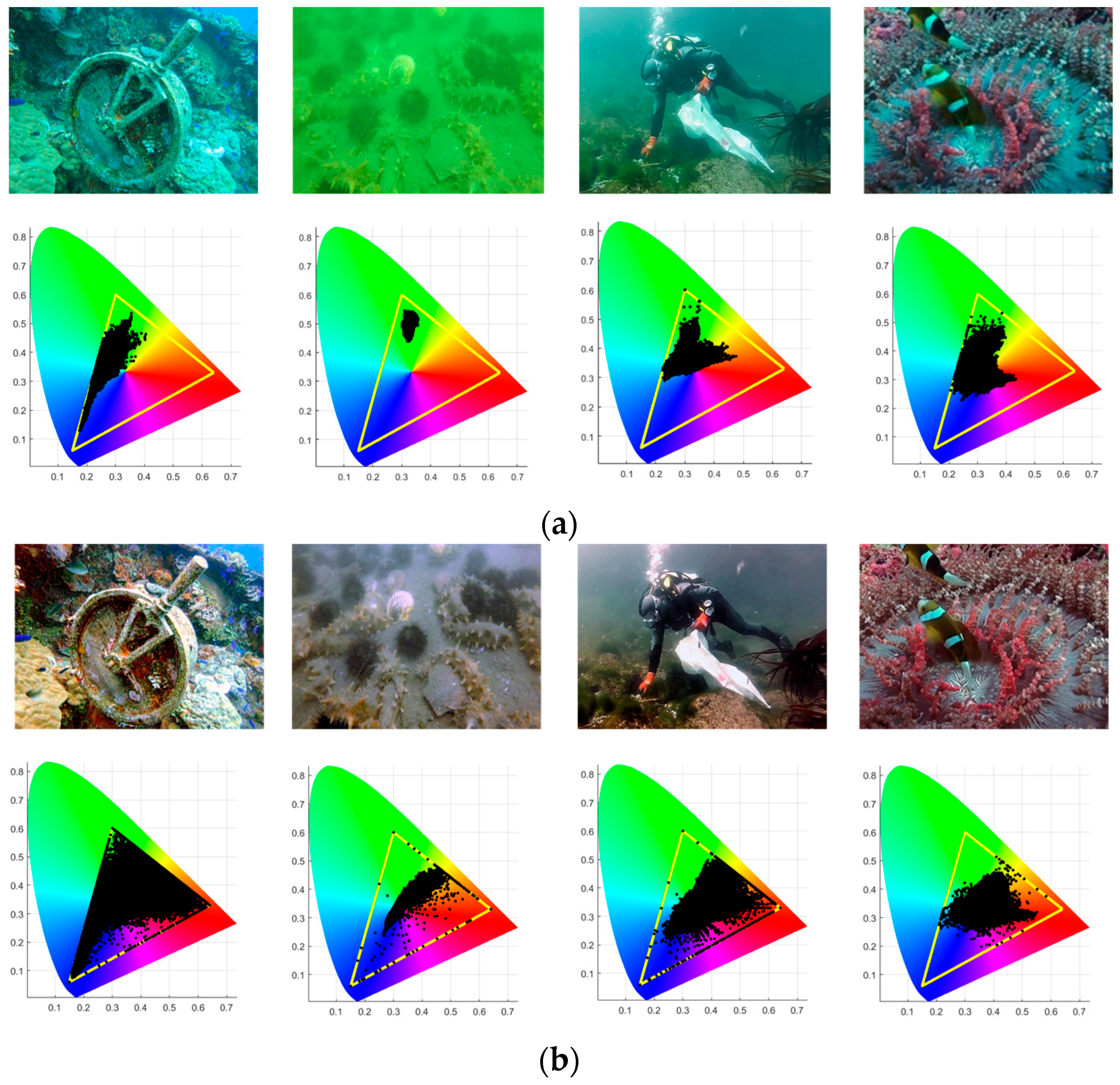
2.1. Color Features of Underwater Images

When objects are observed through the medium of water, they tend to lose part of their color attributes. Underwater images typically have a blue-green background, as if they were filtered through a thick layer of turquoise. The way light behaves in water is significantly different from how it behaves in air. Different wavelengths of light experience varying rates of attenuation underwater. Among the visible wavelengths, red light, with a longer wavelength, is the most weakened. On the other hand, blue-green light, with a wavelength of 480 ± 30 nm, experiences the least amount of absorption, resulting in the greatest penetration underwater, as shown in Figure 2. Due to the RGB camera’s sensitivity to red attenuation, the red component in the captured image appears weak, while the information in the blue and green channels remains relatively intact.

2.2. Gamut Mapping

The color perception of different devices varies due to their respective color ranges, resulting in the same scene appearing in different colors on different devices such as monitors, printers, and cameras. Gamut mapping (GM) is a technique that maps color values from one color space to another, ensuring consistent color across different devices [4]. In digital image processing, GM is commonly used to map an image from the camera’s original color space to the standard RGB or CMYK color space for accurate display or printing of the image. Additionally, GM can also adjust the image’s color saturation, brightness, and contrast properties to achieve better visual effects.

The XYZ color space is designed to represent the human perception system, which is a device-independent color space. The utilization of gamut mapping technology in the XYZ color space can ensure consistent color reproduction across various devices. In addition, the XYZ color space is easily represented in the xy chromaticity diagram, facilitating the gamut comparisons of different images or devices.

In this paper, the principle of GM is applied to map the blue-green color of underwater images to the standard color of air images. The whole process of learning color information in the XYZ space can be expressed as follows:

$${I^{\prime }}_{(x,y,\mathrm{z})}=G(I_{(x,y,\mathrm{z})})$$

(1)

I′_(x,y,z) and I_(x,y,z) represent the color tristimulus values of the underwater image and the normal image, respectively. G is the network that is essential to achieve color mapping between two images. By adjusting the network parameters, different degrees of color mapping can be realized, achieving better visual effects.

2.3. UIE Methods

To improve the quality of underwater images, researchers have developed various algorithms. These algorithms aim to improve visibility and reduce color casts. Based on their foundation in underwater imaging models, existing UIE methods can be divided into the following two categories.

2.3.1. Traditional Methods

Early research in the UIE field focused on using prior knowledge and physical models to estimate the key parameters of underwater imaging models [5]. Since underwater imaging models share similarities with atmospheric scattering models in dehazing tasks [6], some researchers have attempted to extend physics-based dehazing algorithms to underwater scenes. For example, Chiang et al. [7] and Galdran et al. [8] applied the dark channel prior (DCP) dehazing method [9] to underwater image recovery. These methods are primarily concerned with the accurate estimation of media transmission parameters, which is challenging. Therefore, some researchers used the spatial frequency domain method [10,11,12,13,14] to adjust the pixel values of underwater images. Hitam et al. [15] proposed the CLAHE-Mix method, which applies contrast-limited adaptive histogram equalization for UIE. Ancuti et al. [16] proposed a fusion strategy that derived the inputs and the weight measures from the degraded image, enhancing the quality of underwater video and images. Reinhard et al. [17] applied GM to improve image quality by matching the color distribution in the LAB color space. Xiao et al. [18] aligned the gamuts of source and target images through a linear transformation. However, these methods do not consider the underlying imaging mechanisms, and the neglect of the physical degradation process limits improvements in the enhancement quality [19].

2.3.2. Deep Learning Models

Deep learning has made remarkable progress in various advanced computer vision and recognition tasks. Several attempts have been made to improve the performance of UIE through the use of deep learning. Islam et al. [3] utilized a CycleGAN-based approach to construct a large dataset of underwater images and proposed a lightweight conditional GAN for image recovery. Li et al. [20] incorporated features from three color spaces and an attention mechanism, enhancing the network model’s response to regions with severe degradation. Xu et al. [21] proposed an unsupervised adaptive network that enables the training of unpaired underwater images in a GAN model, reducing the dependence on paired datasets for the model. Zhou et al. [22] proposed an underwater multi-feature image enhancement method that incorporates an embedded fusion mechanism to enhance the final reconstruction effect.

However, the aforementioned methods do not take into account the small color gamut caused by the blue-green color bias of underwater images. However, the above method has disadvantages: (1) It does not take into account the visual characteristics of the human eye, so sometimes it cannot provide satisfactory results in color. (2) The small amount of real data makes it difficult to apply to complex and diverse underwater scenes, which limits the performance of UIE. In view of this, we consider the small color gamut in underwater images, and propose a method that combines color gamut mapping and deep learning to accurately map the color gamut range from underwater to normal images, which is more in line with human vision theory. At the same time, we expanded the dataset training, and the model has strong generalization ability and can adapt to various underwater environments.

From the brief review above, our network aims to generate high-visual-quality underwater images by taking into account the unique properties of underwater imaging that change the image’s color gamut.

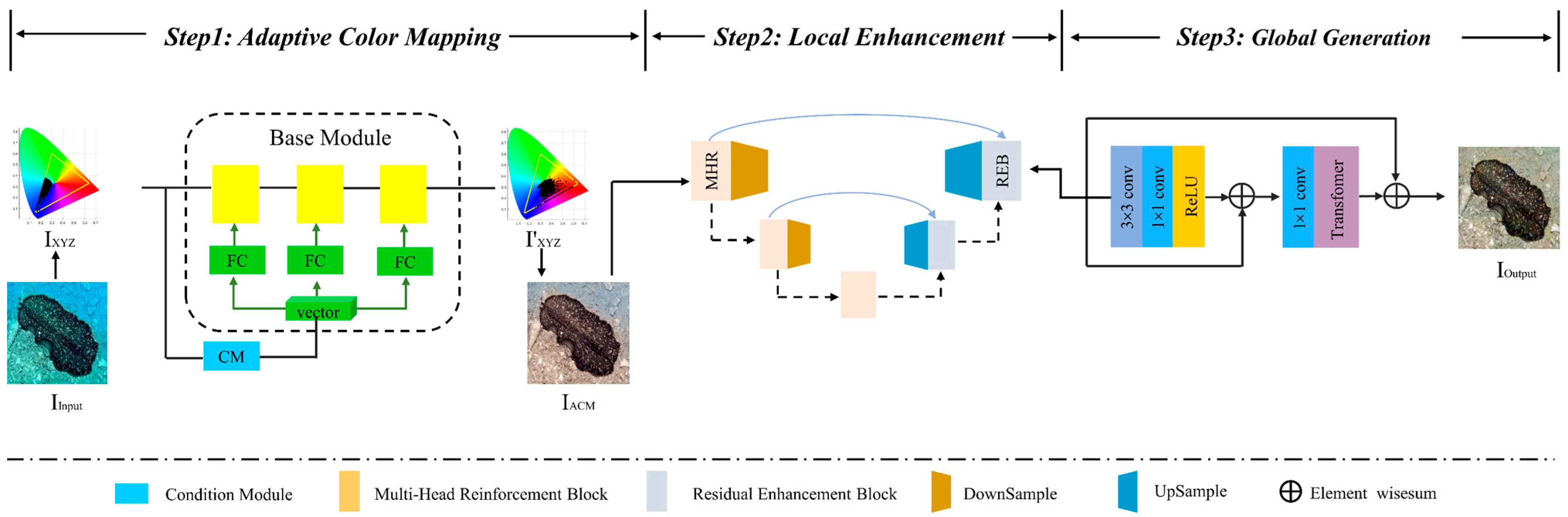
3. The Proposed Method

We present an overview of the architecture of CM-Net in Figure 3—a cascading method consisting of three steps from underwater degraded images to high-quality clear images.

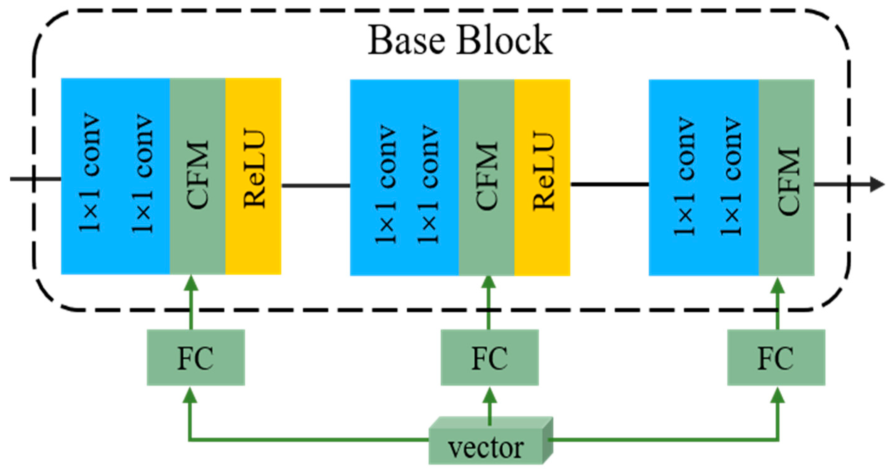
3.1. Adaptive Color Mapping

As the first step, ACM aims to achieve adaptive color correction from underwater degraded images to ground truth.

The XYZ color space is designed to represent the human visual perception system. So, we converted RGB images to XYZ color spaces to represent and process colors in a way that more easily approximated human visual perception. ACM consists of a base module and a condition module, the process of which is described as

$$I_{XYZ}={\mathrm{M}}_1{I}_{RGB}$$

(2)

where M₁ is

$${\mathrm{M}}_1=\left[\begin{array}{l}0.412435 0.357586 0.180423\\ 0.212671 0.715160 0.072169\\ 0.019334 0.119193 0.950227\end{array}\right]$$

(3)

3.1.1. Base Module

The base module is designed to handle global operations, using underwater degradation images as input, with each pixel working independently. It can be described as

$$I_{BM}={\mathrm{F}}_{\mathrm{BM}}(I_{XYZ}(x,y)),\forall (x,y)\in I_{XYZ}$$

(4)

where I_XYZ represents images in the XYZ color space, (x, y) represents the chrominance coordinates in I_XYZ, F_BM denotes the base module, and I_BM represents the output of the base module.

The base module consists of a basic block and the Global Feature Modulation Strategy [23] (GFM), whose specific structure is shown in Figure 4. Thus, the base block is composed of N convolutional layers with 1 × 1 convolutional filters and (N − 1) ReLU activations, which can be denoted as

$${\mathrm{F}}_{\mathrm{BB}}{=(\mathrm{Conv}}_{1\times 1}\circ {\mathrm{Conv}}_{1\times 1}{)}^{\mathrm{N}}\circ {(\mathrm{ReLU}\circ {\mathrm{Conv}}_{1\times 1}(I_{XYZ}\left)\right)}^{\mathrm{N}-1}$$

(5)

The basic block can learn pixel-to-pixel color mapping like a 3D lookup table. Additionally, 1 × 1 filters with multiple layers are good at handling a variety of global operations, while also having the flexibility to adjust feature maps, which is crucial for learning color mapping relationships between images. Liu et al. [24] and Chen et al. [25] also confirmed this view.

To exploit the extracted global color information, we introduce GFM to modulate the intermediate features of the base block, which has been successfully applied in photo retouching and LDR-to-HDR tasks. It can be described as

$$\mathrm{GFM}(x_i)={\alpha }_1\ast x_i+{\alpha }_2$$

(6)

where x_i denotes the feature map. α₁ and α₂ represent the scale and shift factors, respectively.

3.1.2. Conditional Module

To achieve image adaptive mapping, we introduce a conditional module that works in tandem with the base network. The conditional module (CM) primarily focuses on extracting color-related information to enable tunable mapping. As depicted in Figure 5, the CM comprises multiple color feature blocks (CFBs), feature dropouts, convolutional layers, and global average pooling. These components collectively contribute to the system’s ability to enhance and map underwater degradation images accurately.

A color feature block contains two convolution layers with 1 × 1 filters, an average pooling layer, ReLU activation, and layer normalization, which can be written as follows:

$$\mathrm{CFB}(x)=\mathrm{LN}\circ \mathrm{Avgpool}\circ \mathrm{ReLU}\circ \mathrm{SA}\circ {\mathrm{Conv}}_{1\times 1}\circ {\mathrm{Conv}}_{1\times 1}(x)$$

(7)

where x denotes the input of CFB. The condition module takes I_xyz as input and outputs a condition vector V. Our condition module is denoted by

$$V=\mathrm{Avg}\circ {\mathrm{Conv}}_{1\times 1}\circ \mathrm{Dropout}\circ {\mathrm{CFB}}^N(x)$$

(8)

Since the convolutional layer contains only 1 × 1 filters, the conditional module cannot efficiently extract local features. With the help of the pooling layer, the network can extract global priors based on image statistics. A dropout layer is added before the global average pool, which can effectively avoid network overfitting.

The output of ACM is I′_XYZ, which is converted by M₂ to I_ACM, where I_ACM represents the output of ACM. Our goal is to optimize the process of adaptive color correction. M₂ is

$${\mathrm{M}}_2=\left[\begin{array}{l} 3.240479 -1.537150 -0.498535\\ -0.969256 1.875992 0.041556\\ 0.055648 -0.204043 1.057311\end{array}\right]$$

(9)

We can observe the effect of ACM through the CIE chromaticity diagram. As shown in the experimental part, with different images as input to the conditional module, the color gamut changes significantly. The result shows that our ACM implements images adaptively.

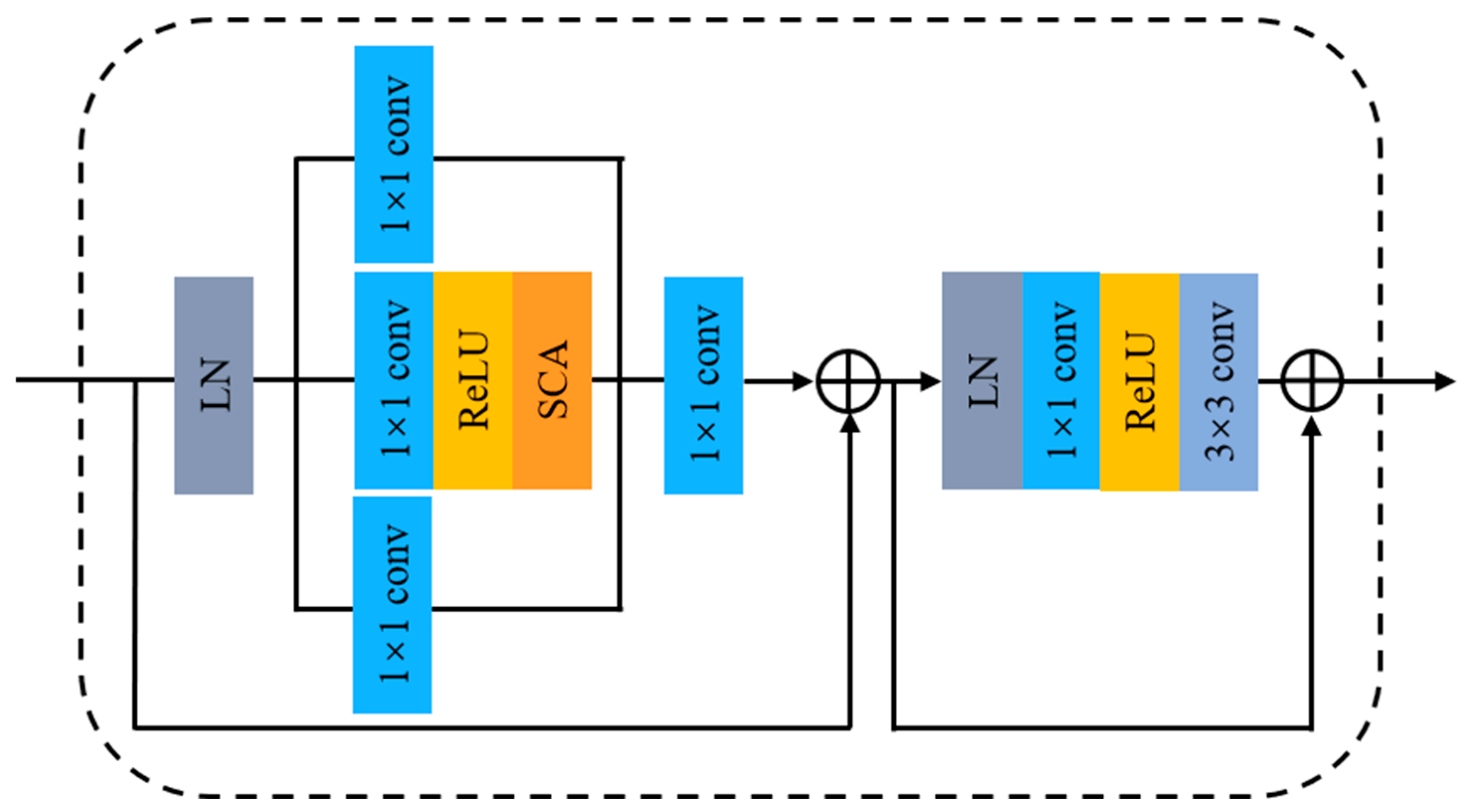
3.2. Local Enhancement

LE is a crucial step performed after ACM to improve the quality of underwater degraded images. ACM can achieve significant improvements, but LE is necessary to bring the results closer to the ground truth. It is worth noting that directly applying local operations for an end-to-end mapping before adaptive color correction often leads to noticeable artifacts in the output results. For detailed information, please refer to the ablation study.

To accomplish LE, we designed a Multi-Head Reinforcement Block (MHR), which is described as follows. This step takes the output of ACM as its input. The features are then passed through a U-shaped encoder–decoder architecture consisting of four down-sampling and up-sampling operations. In the encoder component, MHR is employed to extract features at different scales while doubling the number of feature channels during down-sampling. Conversely, in the decoder component, high-level features are extracted through a Residual Enhancement Block (REB) and then up-sampled to the original size, culminating in the production of the final output. Moreover, skip connections are employed to fuse features from the encoder components to compensate for information loss caused by resampling. Overall, these operations can be represented as

$$I_{LE}=I_{MHR}\circ I_{REB}$$

(10)

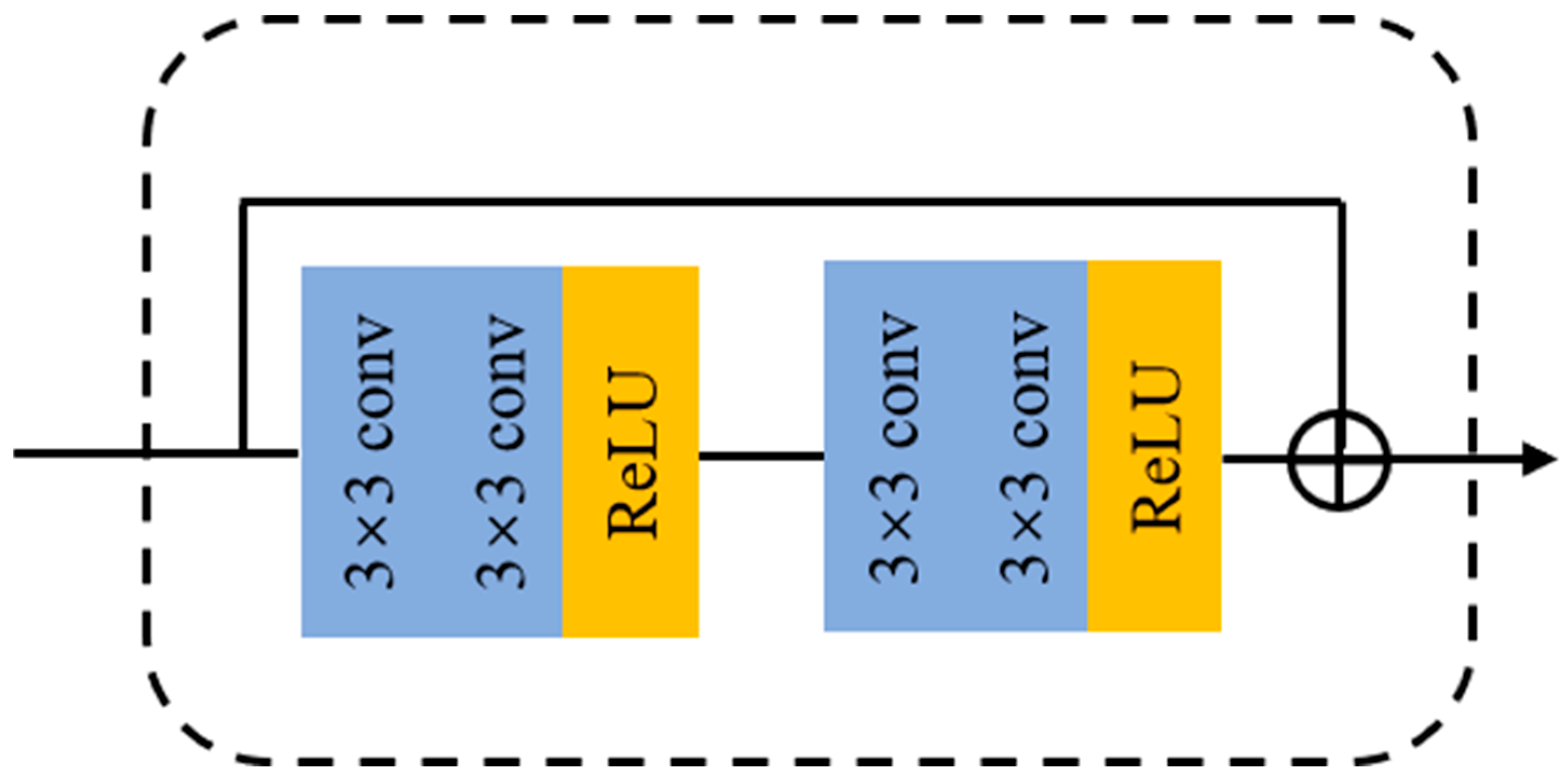
3.2.1. Multi-Head Reinforcement Block

MHR plays a crucial role in learning features at various scales, enabling the in-depth extraction of image information following ACM. It facilitates the recovery of image information from semantic features. The structure of MHR is shown in Figure 6. To realize global information aggregation and channel information interaction between images, we use Simplified Channel Attention (SCA) to help restore missing details of underwater images. As the transformer has flourished and layer normalization (LN) has been used in more and more methods, many studies have shown that using LN can stabilize the training process of the network. SimpleGate simply multiplies features into two parts along the channel dimension, essentially replacing the activation function and reducing the computational complexity within the block. The multi-head structure can realize pixel-level cross-channel context information fusion to recover image details and texture information better.

3.2.2. Residual Enhancement Block

Figure 7 presents the details of the REB, which addresses the issue of vanishing gradients and seeks to maintain data fidelity as much as possible. As the number of filters in the encoder network increases from 64 to 1024, the number of filters in the decoder network decreases from 1024 to 64. Moreover, all convolutional layers within the REB employ a consistent 3 × 3 filter size with a stride of 1. This module ensures coherence and enhances performance in the specific task at hand.

3.3. Global Generation

The third step in our method is GG, which is designed to capture global information that may be overlooked by the local receptive fields of the ACM and LE steps. To effectively capture global information, we introduce a residual–transformer module. It consists of residual learning and transformer blocks. The local residual learning technique bypasses less important information, such as low-resolution regions or low-frequency components. Multiple local residual connections allow the main network to focus its attention on more relevant information.

Additionally, we use the transformer module proposed by the article in [26]. The formulation of this step can be represented as

$$I_{GG}=\mathrm{R}\circ ((I_{TB}\circ {\mathrm{Conv}}_{1\times 1})\circ \mathrm{R}\circ ({\mathrm{Conv}}_{3\times 3}\circ {\mathrm{Conv}}_{1\times 1}\circ (I_{LE})))$$

(11)

where I_TB represents the output of the transformer block, R represents the residual operation, and I_LE stands for the output of LE.

3.4. Loss Function

To recover image details more accurately and capture context information for multiple scale features, we use MSE loss to train the network and optimize weights and biases. The calculation is as follows:

$$L_{MSE}=\frac{1}{N}{\displaystyle \sum _{\mathrm{i}=1}^N{(I_{GT}-I_{Output})}^2}$$

(12)

where N is the number of training images, I_Output is the result of the enhanced underwater image, and I_GT is the ground truth.

4. Experiments and Results

In this section, we first describe the datasets, evaluation metrics, and implementation details. We then present a comparative study involving the proposed method and other enhancement methodologies. Finally, a further analysis of the ablation study is conducted.

4.1. Implementation Details

For training, the input to CMNet is 800 pairs of underwater images in the UIEB dataset [27] and 5050 pairs in the EUVP dark subset [3]. The UIEB dataset includes underwater scenes with low light, color cast, fog, and other underwater degradation features. The EUVP dataset contains a wealth of water types, and the goal is to enhance the perceptual image. For testing, we utilized the remaining 500 synthetic images from a dark subset of the EUVP dataset (denoted as S_500), 90 real-world underwater images from UIEB (denoted as R_90), and 60 challenge images (denoted as C_60) from UIEB. Using a diverse selection of images allows us to evaluate the performance of our model in various scenarios and challenges. Compared to training, we did not resize or randomly crop the input images. We trained our model using ADAM and set the learning rate to 0.0001. The batch size was set to 10, and the epoch number was set to 600. We used Pytorch (Python 3.8) as the deep learning framework on a Linux host with a single NVIDIA GTX 3090Ti GPU (NVIDIA Corp., Santa Clara, CA, USA).

4.2. Experimental Settings

4.2.1. Datasets

The UIEB dataset was proposed by Li et al. in 2019. The UIEB dataset contains a total of 950 pairs of underwater images, of which 890 have corresponding reference images and the remaining 60 images with unsatisfactory reference images are used as challenge data. These images depict different underwater scenes with obvious degradation features such as color coercion, contrast reduction, and detail blurring.

The Euvp dark subset is an EUVP dataset proposed by Islam et al. in 2020, which contains a total of 5550 pairs of images. The data were collected with seven different cameras in different locations under various visibility conditions, Additionally, images extracted from a few publicly available YouTube videos are included in the dataset. The Euvp dataset can adapt to a wide range of natural variations such as scene, water type, and light conditions, enhancing the generalization ability of the model.

4.2.2. Evaluation Metrics

We adopted five commonly used image quality evaluation metrics including peak signal-to-noise ratio (PSNR) [28], structural similarity index measure (SSIM) [29], underwater color image quality evaluation (UCIQE) [30], underwater image quality metric (UIQM) [31], and CIEDE2000 (ΔE00) [32]. A higher PSNR score indicates better image quality for the enhanced image. Similarly, a higher SSIM score indicates a greater similarity between the two images. UCIQE is a composite score that considers color intensity, saturation, and contrast. UIQM consists of three attribute measures: colorfulness, sharpness, and contrast. Higher UIQM/UCIQE scores suggest better visual perception. ΔE00 is employed to quantify the difference between two colors and is considered a highly compatible evaluation method with human vision.

4.2.3. Comparison Methods

Our method was compared with 10 underwater image enhancement methods, including traditional methods—GDCP [33], Red [8], Retinex [34], UDCP [35], and Fusion [16]—as well as deep learning-based methods—F-GAN [3], Water-Net [27], UWCNN [36], U-color [20], and U-Shape [37]. For the traditional methods, we directly applied the methods to the test sets using the authors’ code and training approach. For the deep learning-based methods, we trained them using the author-provided model and network training parameters to ensure an objective experiment.

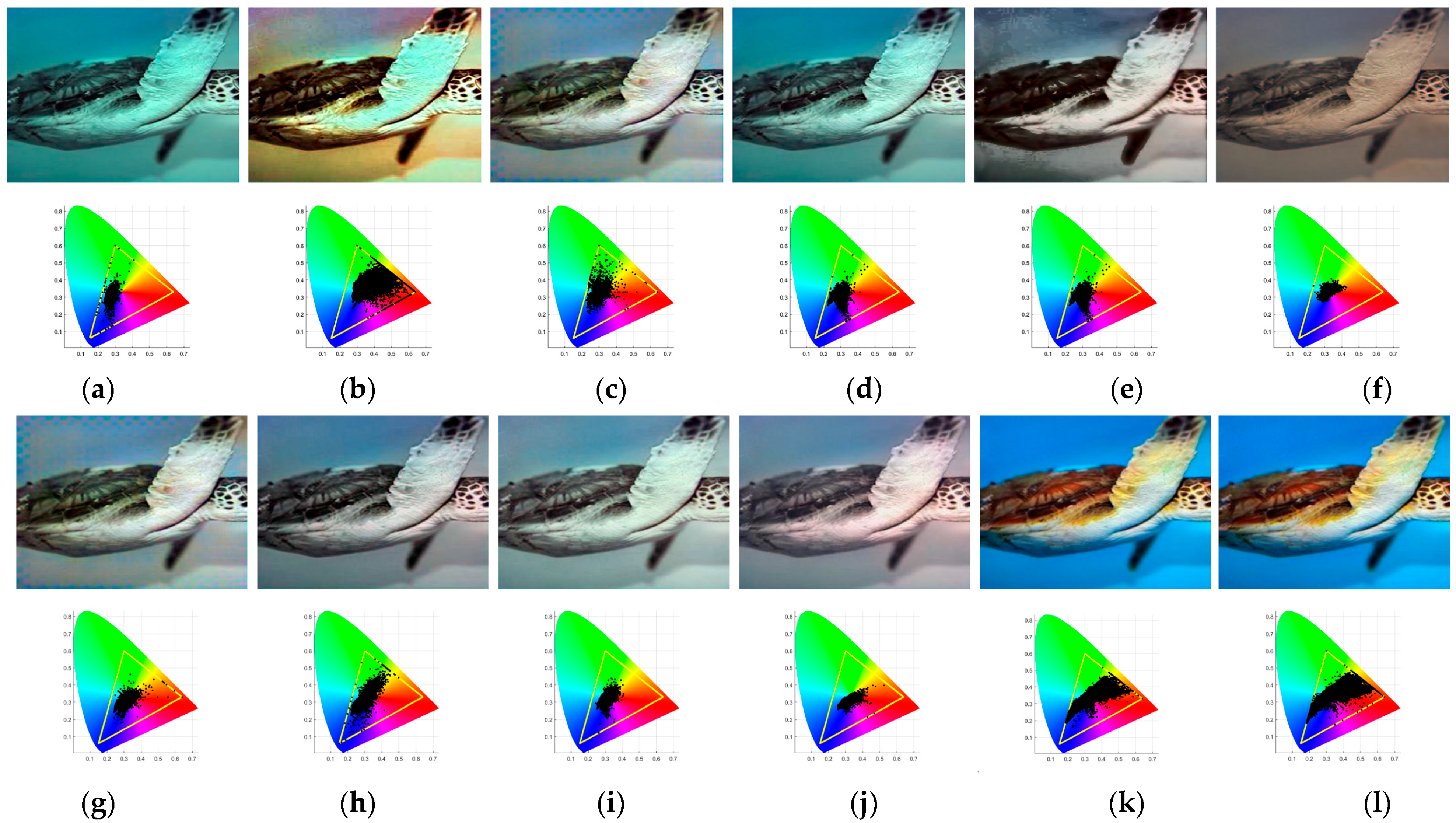
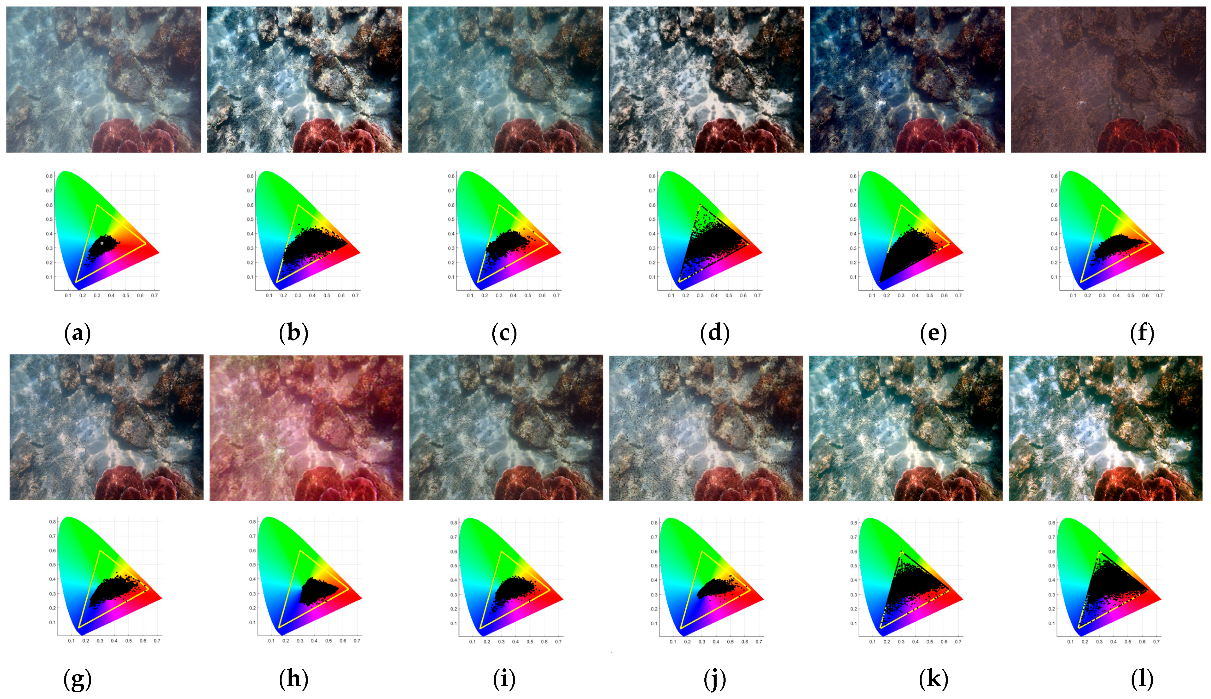
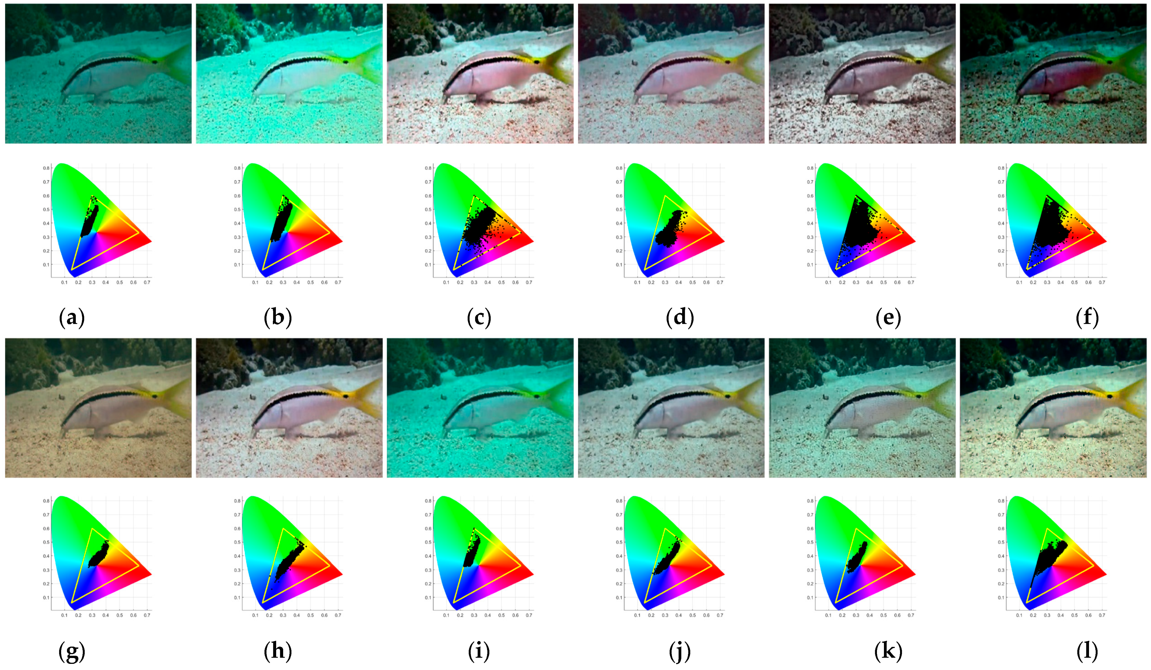
4.3. Visual Comparisons

In this section, we compared our method with other existing methods on diverse testing datasets. Firstly, we evaluated the enhancement effect on a synthetic test set, as shown in Figure 8. It can be observed that the competing methods failed to improve picture contrast or properly correct unwanted color artifacts. None of the compared methods was able to fully restore the scene structure. In contrast, our method achieved the closest results to the ground truth and obtained the highest PSNR and SSIM scores.

Specifically, in Figure 8a, the degraded image exhibited a blue-green deviation. In terms of color correction, GDCP, Red, and F-GAN introduced additional color artifacts. Retinex resulted in oversaturation, and the other methods used for comparison failed to effectively correct the blue-green bias issue.

On the other hand, our proposed method effectively eliminated the blue-green tones, demonstrating the advantages of our designed ACM structure in underwater image enhancement. We then evaluated the results of different methods on real underwater images with a blurry appearance, as depicted in Figure 9. In Figure 9a, the foggy conditions greatly obscured the structural details of the underwater scene. GDCP, UWCNN, and F-GAN produced significant color distortion and highly degraded image quality. Other comparison methods suffered from insufficient image enhancement or introduced oversaturation.

As shown in Figure 10, our method successfully removes the yellow haze and enhances the contrast in the image on the C_60 dataset. In contrast, the Fusion, Retinex, and W-Net methods introduce blue artifacts, while the UWCNN method introduces red artifacts. Our method produces more realistic and clearer image results through effective color correction. This indicates that our method has a significant advantage in improving the quality of underwater images.

Overall, our algorithm successfully eliminates the blurring effect in the image and improves the contrast without introducing noticeable issues of excessive enhancement and oversaturation. These results prominently demonstrate the excellent performance of our method in enhancing the quality and visibility of real underwater images.

4.4. Quantitative Comparisons

In these test datasets, we first conducted quantitative comparisons for R_90 and S_500.

Table 1. Comparison of different methods on S_500 dataset (bold: best).

Method	PSNR	SSIM	UCIQE	UIQM	ΔE00
GDCP	11.71	0.636	0.467	2.30	23.53
Fusion	16.65	0.790	0.446	3.12	16.11
Red	17.87	0.851	0.424	5.15	16.23
Retinex	16.16	0.728	0.411	4.07	16.72
UWCNN	18.19	0.821	0.361	6.47	13.88
W-Net	15.87	0.819	0.410	3.01	19.38
F-GAN	19.93	0.785	0.395	4.42	12.65
U-Color	19.11	0.849	0.380	6.16	13.57
U-Shape	19.18	0.857	0.386	5.72	13.86
CM-Net	22.66	0.908	0.369	5.50	10.31

and

Table 2. Comparison of different methods on R_90 dataset (bold: best).

Method	PSNR	SSIM	UCIQE	UIQM	ΔE00
GDCP	0.735	0.44	3.67	17.77	13.27
Fusion	0.842	0.48	4.46	8.84	20.50
Red	0.814	0.41	5.31	11.93	17.47
Retinex	0.759	0.44	5.09	14.08	17.75
UWCNN	0.680	0.31	7.01	16.30	13.83
W-Net	0.845	0.48	6.10	14.71	19.35
F-GAN	0.734	0.40	5.14	13.69	17.32
U-Color	0.870	0.37	5.58	7.98	20.99
U-Shape	0.800	0.38	6.33	7.88	21.32
CM-Net	0.906	0.45	5.30	7.78	22.71

record the average scores of different methods on PSNR, SSIM, UICQE, UIQM, and ΔE00. According to the results in Table 1, our algorithm outperforms other competing methods in terms of PSNR, SSIM, and ΔE00 metrics. Compared to the second-best method, our CM-Net improves PSNR by 18.1% and 6.5% and SSIM by 5.9% and 13.3% on the S_500 and R_90 datasets, respectively. At the same time, our scores on ΔE00 decreased by 25.6% and 1.3%, respectively.

Since there is no ground truth for C_60, we adopted the no-reference metrics.

Table 3. Comparison of different methods on C_60 dataset (bold: best).

Method	UIQM	UCIQE
GDCP	5.03	0.42
Fusion	5.20	0.48
Red	6.19	0.42
Retinex	6.00	0.42
UDCP	1.37	0.48
UWCNN	7.01	0.32
W-Net	6.34	0.41
F-GAN	4.56	0.39
U-Color	6.84	0.38
U-Shape	4.71	0.39
CM-Net	5.29	0.43

records the average scores of different methods on UIQM and UICQE. Using non-reference image quality evaluation metrics on the three test sets, we found that the UWCNN and Fusion methods excel in UIQM and UCIQE scores. However, visually speaking, UWCNN introduces noticeable red artifacts, greatly diminishing the visual quality of the enhanced images. The Fusion method may not yield satisfactory outcomes in terms of brightness, thereby impacting the overall visual perception of the enhanced images. It is crucial to strike a balance between different image quality metrics and visual aesthetics when evaluating and comparing various image enhancement methods. Our CM-Net’s scores on the test set are slightly inferior to the comparison methods, but, as mentioned by Berman et al. [38] and Ren et al. [39], UIQM and UCIQE are not sensitive to color shifts.

Therefore, we used chromaticity diagrams to visually observe the color distribution of the enhanced images. The chromaticity coordinate of each position on the chromaticity diagram is a quantitative result that describes the physical description of subjective colors of visible light. When the coordinate value of the enhanced image approaches the coordinate of the true color in the chromaticity diagram, the color gamut of the generated results is broader, and the color restoration is more accurate. As shown in Figure 11, Figure 12 and Figure 13, the color range generated by the UWCNN and Fusion methods is relatively small. Additionally, we found some interesting results in our experiments, i.e., that some methods achieve a color gamut beyond or even bigger than the ground-truth color range on the chromaticity diagram, indicating that some competing methods introduce color artifacts or even destroy the intrinsic colors.

4.5. Ablation Study

To demonstrate the effectiveness of each component, we conducted a series of ablation studies on R_90. We carefully considered the components of CM-Net and LE, including ACC, LE, GG, and MHNB. To be more specific, we carried out the following experiments:

• We assessed the positional relationship between the modules. ACC, ACC + LE, and ACC + LE + GG represent combinations of adaptive color mapping, local enhancement, and global generation networks, respectively. CM-Net is the complete model consisting of the three networks ACC, LE, and GG. The LE + ACC + GG model has the local enhancement network positioned in front of the ACC network;
• We assessed the number of MHNBs in LE. The quantities 3 MHNB and 5 MHNB represent the usage of three and five MHNBs, respectively, in the down-sampling process of LE. In CM-Net, four MHNBs are utilized for overall image processing and enhancement.

Statistical results are shown in

Table 4. Ablation study of different components on R_90 dataset (bold: best).

Component	PSNR	SSIM	ΔE00
ACC	20.48	0.867	10.10
ACC + LE	21.43	0.893	8.98
LE + ACC + GG	21.90	0.893	8.67
CM-Net	22.71	0.906	7.98

and

Table 5. Ablation study of different MHRB numbers on R_90 dataset (bold: best).

Component	PSNR	SSIM	ΔE00
3 MHRB	21.61	0.882	9.27
5 MHRB	22.21	0.899	8.69
CM-Net	22.71	0.906	7.98

. Visual comparisons of the effects of each are shown in Figure 14 and Figure 15. The conclusions drawn from the ablation studies are listed as follows:

• As presented in Table 4, our CM-Net achieves the best quantitative performance across two testing datasets when compared with the ablated models, which implies the effectiveness of the combinations of ACC, LE, and GG networks selected in this experiment;
• We experimented with MHRB numbers of {3, 4, 5} in the encoder section. As shown in Table 5, we found that the selected four MHRBs can be the most beneficial to the CM-Net. The results indicate that aimlessly adding the same number of MHNBs will not bring extra performance improvement to enhance underwater images;
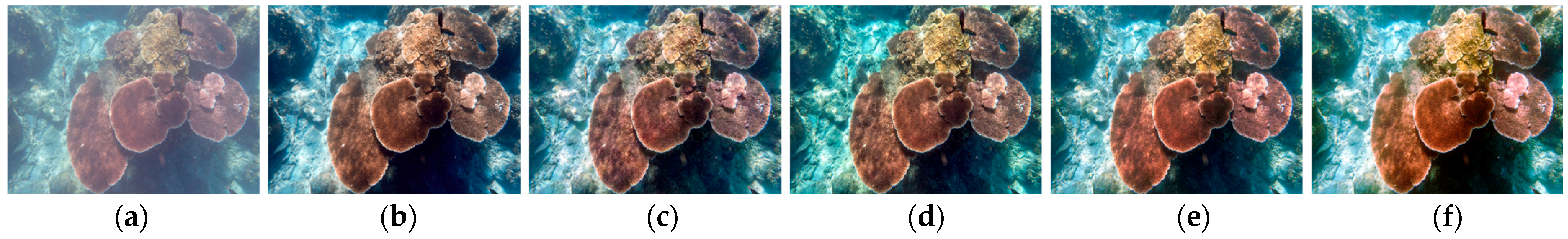
• As shown in Figure 14 and Figure 15, only the images generated by the ACC module have insufficient brightness, and the overall color of the LE enhancement results in front of the ACC network is inaccurate. The five MHNBs may make the network overfit, and the color quality deteriorates instead. The overall color of CM-Net’s results is close to that of the reference image, as LE networks help reconstruct local detail, and GG is good for boosting global brightness. The three modules studied have their functions during the enhancement process, and the combination can improve the overall performance of our network.

5. Conclusions

In this work, we propose a color-mapped underwater image enhancement network. Our model considers human visual perception and employs deep learning techniques to reconstruct underwater images. To address common issues in underwater images such as color artifacts, projection ability, low contrast, and image blur, we have implemented a combination of ACC, LE, and GG modules. The ACC network applies adaptive color mapping, while the MHRB module enables effective feature interaction across multiple scales and preserves fine details. The GG module enhances global highlights. We conducted extensive experiments on various benchmark datasets, demonstrating the superiority of our solution and the effectiveness of the ACC, LE, GG, and MHRB numbers. The results showed that our proposed CMNet outperformed other models by achieving PSNR of 22.66 and 22.71, SSIM of 0.908 and 0.906, and ΔE00 of 10.31 and 7.98 on the EUVP and UIEB datasets. Ablation studies were also conducted to validate the importance of key components in our approach. Looking to the future, considering the evolving needs and advancements in underwater research, we intend to explore lightweight underwater image enhancement models, which will have important implications for real-time operating systems like underwater robotics and monitoring networks.

References

1. Guo, Y.; Li, H.; Zhuang, P. Underwater Image Enhancement Using a Multiscale Dense Generative Adversarial Network. IEEE J. Ocean. Eng. 2020, 45, 862–870. [Google Scholar] [CrossRef]
2. Li, C.Y.; Guo, J.C.; Guo, C.L. Emerging from water: Underwater image color correction based on weakly supervised color transfer. IEEE Signal Process. Lett. 2018, 25, 323–327. [Google Scholar] [CrossRef]
3. Islam, M.J.; Xia, Y.; Sattar, J. Fast Underwater Image Enhancement for Improved Visual Perception. IEEE Robot. Autom. Lett. 2020, 5, 3227–3234. [Google Scholar] [CrossRef]
4. Xu, L.; Zhao, B.; Luo, M.R. Colour gamut mapping between small and large colour gamuts: Part I. gamut compression. Opt. Express 2018, 26, 11481–11495. [Google Scholar] [CrossRef]
5. Mcglamery, B.L. A computer model for underwater camera systems. Proc. SPIE 1980, 208, 221–231. [Google Scholar]
6. Akkaynak, D.; Treibitz, T. Sea-Thru: A Method for Removing Water from Underwater Images. In Proceedings of the 2019 IEEE/CVF Conference on Computer Vision and Pattern Recognition (CVPR), Long Beach, CA, USA, 15–20 June 2019; pp. 1682–1691. [Google Scholar]
7. Chiang, J.Y.; Chen, Y.C. Underwater Image Enhancement by Wavelength Compensation and Dehazing. IEEE Trans. Image Process. 2012, 21, 1756–1769. [Google Scholar] [CrossRef] [PubMed]
8. Galdran, A.; Pardo, D.; Picón, A.; Alvarez-Gila, A. Automatic Red-Channel underwater image restoration. J. Vis. Commun. Image Represent. 2015, 26, 132–145. [Google Scholar] [CrossRef]
9. HE, K.M.; Sun, J.; Tang, X.O. Single Image Haze Removal Using Dark Channel Prior. IEEE Trans. Pattern Anal. Mach. Intell. 2011, 33, 2341–2353. [Google Scholar] [PubMed]
10. Robert, H. Image enhancement by histogram transformation. Comput. Graph. Image Process. 1977, 6, 184–195. [Google Scholar]
11. Stephen, M.P.; Philip, A.E.; John, D.A.; Robert, C.; Ari, G.; Trey, G.; Bart, T.H.R.; John, B.Z.; Karel, Z. Adaptive histogram equalization and its variations. Comput. Vis. Graph. Image Process. 1987, 39, 355–369. [Google Scholar]
12. Liu, Y.C.; Chan, W.H.; Chen, Y.Q. Automatic white balance for digital still camera. IEEE Trans. Consum. Electron. 2002, 41, 460–466. [Google Scholar]
13. Land, E.H. The Retinex Theory of Color Vision. Sci. Am. 1978, 237, 108–128. [Google Scholar] [CrossRef] [PubMed]
14. Land, E.H. An alternative technique for the computation of the designator in the retinex theory of color vision. Proc. Natl. Acad. Sci. USA 1986, 83, 3078–3080. [Google Scholar] [CrossRef]
15. Hitam, M.S.; Awalludin, E.A.; Jawahir, H.W.; Yussof, W.N.; Bachok, Z. Mixture contrast limited adaptive histogram equalization for underwater image enhancement. In Proceedings of the 2013 International Conference on Computer Applications Technology (ICCAT), Sousse, Tunisia, 20–22 January 2013; pp. 1–5. [Google Scholar]
16. Ancuti, C.; Ancuti, C.O.; Haber, T.; Bekaert, P. Enhancing underwater images and videos by fusion. In Proceedings of the 2012 IEEE Conference on Computer Vision and Pattern Recognition, Providence, RI, USA, 16–21 June 2012; pp. 81–88. [Google Scholar]
17. Reinhard, E.; Adhikhmin, M.; Gooch, B.; Shirley, P. Color transfer between images. IEEE Comput. Graph. Appl. 2001, 21, 34–41. [Google Scholar] [CrossRef]
18. Xiao, X.Z.; Ma, L.Z. Color transfer in correlated color space. In Proceedings of the 2006 ACM International Conference on Virtual Reality Continuum and Its Applications (VRCIA’06), New York, NY, USA, 12–26 June 2006; pp. 305–309. [Google Scholar]
19. Liu, R.S.; Fan, X.; Zhu, M.; Hou, M.J.; Luo, Z.X. Real-World Underwater Enhancement: Challenges, Benchmarks, and Solutions Under Natural Light. IEEE Trans. Circuits Syst. Video Technol. 2020, 30, 4861–4875. [Google Scholar] [CrossRef]
20. Li, C.Y.; Anwar, S.; Hou, J.H.; Cong, R.M.; Guo, C.L.; Ren, W.Q. Underwater image enhancement via medium transmission-guided multi-color space embedding. IEEE Trans. Image Process. 2021, 30, 4985–5000. [Google Scholar] [CrossRef] [PubMed]
21. Ye, X.C.; Li, Z.P.; Sun, B.L.; Wang, Z.H.; Xu, R.; Li, H.J.; Fan, X. Deep Joint Depth Estimation and Color Correction from Monocular Underwater Images Based on Unsupervised Adaptation Networks. IEEE Trans. Circuits Syst. Video Technol. 2020, 30, 3995–4008. [Google Scholar] [CrossRef]
22. Zhou, J.C.; Sun, J.M.; Zhang, W.S.; Lin, Z.F. Multi-view underwater image enhancement method via embedded fusion mechanism. Eng. Appl. Artif. Intell. 2023, 121, 105946. [Google Scholar] [CrossRef]
23. He, J.; Liu, Y.; Qiao, Y.; Dong, C. Conditional Sequential Modulation for Efficient Global Image Retouching. In Proceedings of the Computer Vision—ECCV 2020: 16th European Conference, Glasgow, UK, 23–28 August 2020; pp. 679–695. [Google Scholar]
24. Liu, Y.H.; He, J.W.; Chen, X.Y.; Zhang, Z.W.; Zhao, H.Y.; Dong, C.; Qiao, Y. Very Lightweight Photo Retouching Network with Conditional Sequential Modulation. IEEE Trans. Multimed. 2022, 25, 4638–4652. [Google Scholar] [CrossRef]
25. Chen, X.Y.; Zhang, Z.W.; Ren, J.S.; Tian, L.; Qiao, Y.; Dong, C. A New Journey from SDRTV to HDRTV. In Proceedings of the 2021 IEEE/CVF International Conference on Computer Vision (ICCV), Montreal, QC, Canada, 10–17 October 2021; pp. 4480–4489. [Google Scholar]
26. Zamir, S.W.; Arora, A.; Khan, S.; Hayat, M.; Khan, F.S.; Yang, M.H. Restormer: Efficient Transformer for High-Resolution Image Restoration. In Proceedings of the 2022 IEEE/CVF Conference on Computer Vision and Pattern Recognition (CVPR), New Orleans, LA, USA, 18–24 June 2022; pp. 5718–5729. [Google Scholar]
27. Li, C.Y.; Guo, C.L.; Ren, W.Q.; Cong, R.M.; Hou, J.H.; Kwong, S.; Tao, D.C. An underwater image enhancement benchmark dataset and beyond. IEEE Trans. Image Process. 2019, 29, 4376–4389. [Google Scholar] [CrossRef]
28. Korhonen, J.; You, J. Peak signal-to-noise ratio revisited: Is simple beautiful? In Proceedings of the 2012 Fourth International Workshop on Quality of Multimedia Experience, Melbourne, VIC, Australia, 5–7 July 2012; pp. 37–38. [Google Scholar]
29. Zhou, W.; Bovik, A.C.; Sheikh, H.R.; Simoncelli, E.P. Image quality assessment: From error visibility to structural similarity. IEEE Trans. Image Process. 2004, 13, 600–612. [Google Scholar]
30. Yang, M.; Sowmya, A. An underwater color image quality evaluation metric. IEEE Trans. Image Process. 2015, 24, 6062–6071. [Google Scholar] [CrossRef] [PubMed]
31. Tao, Y.; Dong, L.L.; Xu, W.H. A novel two-step strategy based on white-balancing and fusion for underwater image enhancement. IEEE Access 2020, 8, 217651–217670. [Google Scholar] [CrossRef]
32. Sharma, G.; Wu, W.C.; Dalal, E.N. The CIEDE2000 color-difference formula: Implementation notes, supplementary test data, and mathematical observations. Color Res. Appl. 2005, 30, 21–30. [Google Scholar] [CrossRef]
33. Peng, Y.T.; Cao, K.M.; Cosman, P.C. Generalization of the dark channel prior for single image restoration. IEEE Trans. Image Process. 2018, 27, 2856–2868. [Google Scholar] [CrossRef]
34. Fu, X.Y.; Zhuang, P.X.; Huang, Y.; Liao, Y.H.; Zhang, X.P.; Ding, X.H. A retinex-based enhancing approach for single underwater image. In Proceedings of the 2014 IEEE International Conference on Image Processing (ICIP), Paris, France, 27–30 October 2014; pp. 4572–4576. [Google Scholar]
35. Drews, P., Jr.; do Nascimento, E.; Moraes, F.; Botelho, S.; Campos, M. Transmission estimation in underwater single images. In Proceedings of the IEEE International Conference on Computer Vision Workshops, Sydney, NSW, Australia, 2–8 December 2013; pp. 825–830. [Google Scholar]
36. Li, C.Y.; Anwar, S.; Porikli, F. Underwater scene prior inspired deep underwater image and video enhancement. Pattern Recognit. 2020, 98, 107038. [Google Scholar] [CrossRef]
37. Peng, L.T.; Zhu, C.L.; Bian, L.H. U-Shape Transformer for Underwater Image Enhancement. IEEE Trans. Image Process. 2023, 32, 3066–3079. [Google Scholar] [CrossRef]
38. Berman, D.; Levy, D.; Avidan, S.; Treibitz, T. Underwater Single Image Color Restoration Using Haze-Lines and a New Quantitative Dataset. IEEE Trans. Pattern Anal. Mach. Intell. 2021, 43, 2822–2837. [Google Scholar] [CrossRef]
39. Ren, T.D.; Xu, H.Y.; Jiang, G.Y.; Yu, M.; Zhang, X.; Wang, B.; Luo, T. Reinforced Swin-Convs Transformer for Underwater Image Enhancement. IEEE Trans. Geosci. Remote Sens. 2022, 60, 1–16. [Google Scholar]
Figure 1. The comparison of underwater and normal images: (a) underwater image and corresponding chromaticity diagram; (b) normal images and corresponding chromaticity diagram.
Mathematics 12 01933 g001
Figure 2. The diagram of underwater light attenuation.
Mathematics 12 01933 g002
Figure 3. The architecture of the proposed CM-Net.
Mathematics 12 01933 g003
Figure 4. The architecture of the base module.
Mathematics 12 01933 g004
Figure 5. The architecture of the conditional module.
Mathematics 12 01933 g005
Figure 6. The architecture of the MHR.
Mathematics 12 01933 g006
Figure 7. The architecture of the REB.
Mathematics 12 01933 g007
Figure 8. Visual comparison on the S_500 dataset: (a) raw; (b) GDCP; (c) Fusion; (d) Red; (e) Retinex; (f) UWCNN; (g) W-Net; (h) F-GAN; (i) U-color; (j) U-Shape; (k) CM-Net; (l) ground truth.
Mathematics 12 01933 g008
Figure 9. Visual comparison on the R_90 dataset: (a) raw; (b) GDCP; (c) Fusion; (d) Red; (e) Retinex; (f) UWCNN; (g) W-Net; (h) F-GAN; (i) U-color; (j) U-Shape; (k) CM-Net; (l) ground truth.
Mathematics 12 01933 g009
Figure 10. Visual comparison on the C_60 dataset: (a) raw; (b) GDCP; (c) Fusion; (d) Red; (e) Retinex; (f) UDCP; (g) UWCNN; (h) W-Net; (i) F-GAN; (j) U-color; (k) U-Shape; (l) CM-Net.
Mathematics 12 01933 g010
Figure 11. Visual comparison and corresponding chromaticity diagram on the S_500 dataset: (a) raw; (b) GDCP; (c) Fusion; (d) Red; (e) Retinex; (f) UWCNN; (g) W-Net; (h) F-GAN; (i) U-color; (j) U-Shape; (k) CM-Net; (l) ground truth.
Mathematics 12 01933 g011
Figure 12. Visual comparison and corresponding chromaticity diagram on the R_90 dataset: (a) raw; (b) GDCP; (c) Fusion; (d) Red; (e) Retinex; (f) UWCNN; (g) W-Net; (h) F-GAN; (i) U-color; (j) U-Shape; (k) CM-Net; (l) ground truth.
Mathematics 12 01933 g012
Figure 13. Visual comparison and corresponding chromaticity diagram on the C_60 dataset: (a) raw; (b) GDCP; (c) Fusion; (d) Red; (e) Retinex; (f) UDCP; (g) UWCNN; (h) W-Net; (i) F-GAN; (j) U-color; (k) U-Shape; (l) CM-Net.
Mathematics 12 01933 g013
Figure 14. Visual comparison of different components on R_90 dataset: (a) raw; (b) ACC; (c) ACC + LE; (d) LE + ACC + GG; (e) CM-Net; (f) ground truth.
Mathematics 12 01933 g014
Figure 15. Visual comparison of different MHRB numbers on R_90 dataset: (a) raw; (b) 3 MHRB; (c) 5 MHRB; (d) CM-Net; (e) ground truth.
Mathematics 12 01933 g015