Exact Periodic Wave Solutions for the Perturbed Boussinesq Equation with Power Law Nonlinearity

Abstract

In this paper, exact periodic wave solutions for the perturbed Boussinesq equation with power law nonlinearity are obtained for different nonlinear strengths n. When $n=1$, the periodic traveling wave solutions can be found by the definition of the Jacobian elliptic function. When $n\ge 1$, we construct a transformation to solve for the power law nonlinearity, and the periodic traveling wave solutions can be obtained by applying the extended trial equation method. In addition, we consider the limiting case where the periodicity of the periodic traveling wave solutions vanishes, and we obtain the soliton solution for $n=1$. Numerical simulations show the periodicity of the solution for the perturbed Boussinesq equation.

1. Introduction

The Boussinesq equations are most commonly used to describe the propagation of small amplitude, plane, and long waves over water. The Boussinesq equations are perturbations of the linear wave equation that consider the small effects of nonlinearity and dispersion. In 1872, Joseph Boussinesq first derived the Boussinesq Equation [1]

$${\mu }_{tt}-b_0{c}_0{\mu }_{xx}=b_0{c}_0{\left(\frac{3}{2c_0}{\mu }^2+\frac{{c_0}^2}{3}{\mu }_{xx}\right)}_{xx},$$

where $\mu (x,t)$ represents the non-perturbed surface, with x and t indicating the spatial and temporal coordinates, respectively. $b_0$ is the gravitational constant, and $c_0$ is the depth averaged over the surface. In non-dimensional units, the Boussinesq equations can be written as follows:

$${\mu }_{tt}-{\mu }_{xx}+{({\mu }^2)}_{xx}+{\mu }_{xxxx}=0.$$

(1)

From (1), it can be seen that both ${\mu }_{tt}$ and ${\mu }_{xxxx}$ have the same sign. The Boussinesq equations with this characteristic are often called the good Boussinesq equations, and equations with the opposite characteristic are called the bad Boussinesq equations, as follows:

$${\mu }_{tt}-{\mu }_{xx}-{({\mu }^2)}_{xx}-{\mu }_{xxxx}=0.$$

(2)

It is worth noting that the terms ${\mu }_{tt}$ and ${\mu }_{xxxx}$ have the opposite signs.

In this study, we consider the following perturbed Boussinesq equation with power law nonlinearity

$$u_{tt}-d^2{u}_{xx}+a{(u^{2n})}_{xx}+b{u}_{xxxx}=\beta u_{xx}+\rho u_{xxxx},$$

(3)

where $u(x,t)$ denotes the waveform, n is the strength of nonlinearity, and d, a, b, $\beta$, and $\rho$ are real-valued constants $(-d^2\ne \beta$, $b\ne \rho$, and $a\ne 0)$. Equation (3) was initially introduced by Anjan Biswas et al. [2]. The coefficient $\beta$ affects the dissipative term, while the coefficient $\rho$ provides higher-order stability. The terms $\beta$ and $\rho$ represent perturbations, and their presence affects the positivity of $u_{xx}$, and $u_{xxxx}$. When $d=1$, $a=1$, $b=1$, $\beta =\rho =0$, and $n=1$ in Equation (3), it represents the classical Boussinesq equation. This paper studies the Boussinesq equation with general n and non-zero $\beta$ and $\rho$. On the left side of Equation (3), $a{(u^{2n})}_{xx}$ represents the nonlinear term. Equation (3) contains three types of equations:

(1)

when $d^2+\beta >0$ and $b-\rho >0$, Equation (3) represents a good Boussinesq equation;

(2)

when $d^2+\beta >0$ and $b-\rho <0$, Equation (3) represents a bad Boussinesq equation;

(3)

when $d^2+\beta <0$, Equation (3) represents neither a good nor bad Boussinesq equation.

The perturbed Boussinesq equations have distinct mathematical properties due to the positive and negative nature of $d^2+\beta$ and $b-\rho$. The good Boussinesq equation has been widely studied in the existing literature, covering the local and global well posedness to the solutions of initial value problems [3,4]. However, the situation is the opposite for the bad Boussinesq equation, which is almost always likely to be not well posed [5].

The good Boussinesq equation describes a two-dimensional non-rotational flow of a viscous fluid in a homogeneous rectangular channel. In recent years, it has been studied in many different aspects. Xu et al. studied the Cauchy problem of the solutions for the good Boussinesq equation with three different initial energy levels [6]. Charlier et al. established the asymptotic behavior of the solutions for the good Boussinesq Equation [7]. In [8], Luigi obtained numerical solutions for the good Boussinesq equation. The bad Boussinesq equation describes the two-dimensional flow of small amplitude shallow water waves. It is closely related to the dynamics of the anharmonic lattice in the Fermi–Pasta–Ulam (FPU) problem [9]. In [5], the local generalized solutions of the bad Boussinesq equation have been shown under a mild condition for the initial data. The non-existence of weak solutions for the initial boundary value problem was investigated in [10]. Dai et al. studied the explicit homoclinic orbit and the solitons for the bad Boussinesq equation with periodic boundary conditions [11]. The blow-up solutions for the bad Boussinesq equation were found in [12].

Solving nonlinear partial differential equations (PDEs) is an important area of research within the field of nonlinear evolution equations. This branch of research is valuable for helping scientists comprehend complex physical phenomena. There are a large number of methods for obtaining exact solutions of nonlinear evolution Equations [13,14,15,16,17,18,19,20]. In [13], the dynamical systems method was proposed for the modified Zakharov equations with a quantum correction. In order to obtain new types of solutions, Benjamin investigated the positive-operator method [14]. The generalized Zakharov–Kuznetsov equation was solved using the F-expansion method in [15]. The Gardner equation was solved using the Exp-function method by Wang et al. in [16]. In [17], Hulya presented the trigonometric type of solutions to nonlinear Schrödinger’s equation using the $(G^{\prime }/G)$ expansion method. The authors obtained the exact solutions of the nonlinear evolution equation utilizing the Bäcklund method [18]. Sivalingam et al. studied the fractional differential equations by the neural network scheme in [19,20].

In recent years, little research has been conducted on the solutions of the perturbed Boussinesq Equation (3) [2,21,22]. Anjan Biswas obtained the solitary wave solutions for (3) with $\beta =\rho =0$ by the ansatz method [2]. The mapping method was employed to derive the exact 1-soliton solution and the singular solution for (3) with $n=1$[21]. In [22], the authors also studied the soliton solutions for (3) with $n=1$ using the modified auxiliary equation method. However, they only obtained solitary wave solutions for (3). No relevant work has been carried out on the periodic wave solutions for the perturbed Boussinesq Equation (3). As is well-known, the periodic wave solutions of nonlinear evolution equations are widely found in daily life, such as tidal phenomena, animal reproduction, food supply, plant growth, seasonal changes, and so on. The investigation of the periodic solutions to (3) not only extends the form of the exact traveling wave for the perturbed Boussinesq equation but also lays the foundation for researchers to study the qualitative analysis for the perturbed Boussinesq equation in the future, such as the stability. The main contributions of this paper are as follows:

• The exact periodic wave solutions for the perturbed Boussinesq equation with power law nonlinearity are studied. To the best of the authors’ knowledge, it is the first time to explore periodic wave solutions for the perturbed Boussinesq equation. Moreover, the periodic traveling wave solutions of the perturbed Boussinesq equation are obtained for general n, not just for a specific value of n [21,22].
• Different from the existing periodic wave solutions [15,16,17] for nonlinear evolution equations, which are expressed in trigonometric functions [15,17] and exponential functions [16]. The periodic solutions for the perturbed Boussinesq equation in this paper are expressed in terms of Jacobian elliptic functions. The Jacobian elliptic function is more suitable for engineering applications than other functions, such as the Duffing system, which is often used to describe oscillations in circuit systems [23].
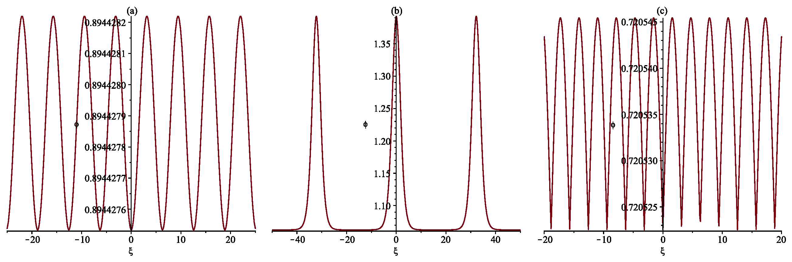
• Furthermore, we investigate the limiting case where the periodicity of the periodic traveling wave solution vanishes and derive the soliton solution with a single-peaked waveform.

The remainder of this paper is arranged as follows. Section 2 introduces the definition of the Jacobian elliptic function and its related properties. Section 3 shows the periodic traveling wave solutions of the perturbed Boussinesq Equation (3) in two cases ($n=1$ and $n\ge 1$). The simulation results are presented to illustrate the periodicity of three types of Boussinesq equations in Section 4. The paper is concluded in Section 5.

2. Preliminaries

In this section, we introduce Jacobian elliptic functions. We refer the reader to the book Jaime [24] as the reference to this theory. There are three basic Jacobian elliptic functions, $cn(u,h)$, $dn(u,h)$, and $sn(u,h)$, where h is the elliptic modulus. We start with the definition of the normal elliptic integral of the first kind

$$F(\varphi ,h)\equiv u={\int }_0^{\varphi }\frac{dt}{\sqrt{1-h^{2}si{n}^{2}t}},$$

where $0<h^2<1$ and $\varphi =am(u,h)=am(u)$ is the Jacobi amplitude. We denote

$$F^{-1}(\varphi ,h)=\varphi =am(u,h).$$

Further steps can be obtained:

$$sin\varphi =sin(am(u,h))=sn(u,h),$$

$$cos\varphi =cos(am(u,h))=cn(u,h),$$

$$\sqrt{1-h^{2}si{n}^2\varphi }=\sqrt{1-h^{2}si{n}^2(am(u,h))}=dn(u,h).$$

Based on the literature [24], the basic properties of the above three types of Jacobian elliptic functions are as follows:

$$\left\{\begin{array}{c}s{n}^{2}u+c{n}^{2}u=1,h^{2}s{n}^{2}u+d{n}^{2}u=1,\hfill \\ sn(u+2K(h),h)=-sn(u,h),cn(u+2K(h),h)=-cn(u,h),dn(u+2K(h),h)=dn(u,h),\hfill \\ -1\le cnu\le 1,-1\le snu\le 1,h^{\prime }\le dnu\le 1,\hfill \end{array}\right.$$

where $h^{\prime }=\sqrt{1-h^2}$ is a replenishment modulus and $K(h)=F(\pi /2,h)$ is the complete elliptic integral of the first type.

3. Exact Periodic Wave Solutions for the Perturbed BE

We use the following traveling wave transformation:

$$u(x,t)=\varphi (\xi ),\xi =x-ct.$$

(4)

Inserting (4) into Equation (3) and integrate the equation with respect to $\xi$ twice, we obtain

$$(c^2-d^2-\beta )\varphi +a({\varphi }^{2n})+(b-\rho ){\varphi }^{″}=A_{\varphi },$$

(5)

with ${\varphi }^{″}=\frac{{\partial }^2\varphi }{\partial {\xi }^2}$, and where $A_{\varphi }$ is the integration constant. The nonlinear term ${\varphi }^{2n}$ in (5) is difficult to derive directly, and we discuss it separately for the two cases $n=1$ and $n\ge 1$ using both direct and indirect methods. In the next sub-sections, we discuss the periodic solutions for two cases: $n=1$ and $n\ge 1$.

3.1. n = 1 in Equation (3)

In this sub-section, we discuss the case of the equation at $n=1$. When $n=1$, Equation (5) can be rewritten as follows:

$$(c^2-d^2-\beta )\varphi +a({\varphi }^2)+(b-\rho ){\varphi }^{″}=A_{\varphi }.$$

(6)

We multiply (6) by the integrating factor ${\varphi }^{\prime }$, and we integrate once more for $\xi$

$$\frac{1}{2}(c^2-d^2-\beta ){\varphi }^2+\frac{a}{3}{\varphi }^3+\frac{b-\rho }{2}{({\varphi }^{\prime })}^2=A_{\varphi }\varphi +B_{\varphi },$$

(7)

where $B_{\varphi }$ is another constant of integration. This simplifies to

$$\begin{array}{cc}\hfill {({\varphi }^{\prime })}^2& =-\frac{2a}{3(b-\rho )}{\varphi }^3-\frac{c^2-d^2-\beta }{b-\rho }{\varphi }^2+A_{\varphi }\varphi +B_{\varphi }\hfill \\ \hfill & =\frac{2a}{3(b-\rho )}[-{\varphi }^3-\frac{3(c^2-d^2-\beta )}{2a}{\varphi }^2+\frac{3(b-\rho )}{2a}{A}_{\varphi }\varphi +\frac{3(b-\rho )}{2a}{B}_{\varphi }].\hfill \end{array}$$

(8)

Formula (8) can be rewritten as

$${({\varphi }^{\prime })}^2=\frac{2a}{3(b-\rho )}F(\varphi ),$$

(9)

with $F(\varphi )=-{\varphi }^3-\frac{3(c^2-d^2-\beta )}{2a}{\varphi }^2+\frac{3(b-\rho )}{2a}{A}_{\varphi }\varphi +\frac{3(b-\rho )}{2a}{B}_{\varphi }$. Let ${\alpha }_1$, ${\alpha }_2$, and ${\alpha }_3$ be the non-zero roots of the polynomial $F(\varphi )$, such that the polynomial

$$F(\varphi )=(\varphi -{\alpha }_1)(\varphi -{\alpha }_2)({\alpha }_3-\varphi )$$

(10)

is obtained. Without loss of generality, we assume that ${\alpha }_1<{\alpha }_2<{\alpha }_3$. From (8), we can deduce that

$$\left\{\begin{array}{c}{\alpha }_1+{\alpha }_2+{\alpha }_3=-\frac{3(c^2-d^2-\beta )}{2a},\hfill \\ {\alpha }_1{\alpha }_2+{\alpha }_1{\alpha }_3+{\alpha }_2{\alpha }_3=\frac{3(b-\rho )}{2a}{A}_{\varphi },\hfill \\ {\alpha }_1{\alpha }_2{\alpha }_3=\frac{3(b-\rho )}{2a}{B}_{\varphi }.\hfill \end{array}\right.$$

(11)

We denote $\phi =\frac{\varphi }{{\alpha }_3}$. Then, substituting it into (8) and (10), we obtain

$${({\phi }^{\prime })}^2=\frac{2a{\alpha }_3}{3(b-\rho )}(\phi -{\eta }_1)(\phi -{\eta }_2)(1-\phi ),$$

(12)

where ${\eta }_i=\frac{{\alpha }_i}{{\alpha }_3}$, $i=1$, 2. Moreover, we define a new variable $\psi$, which satisfies $\phi =1+({\eta }_2-1)si{n}^2\psi$. Substituting it into (12), after some more calculations, we obtain

$${({\psi }^{\prime })}^2=\frac{a{\alpha }_3}{6(b-\rho )}(1-{\eta }_1)(1-\frac{1-{\eta }_2}{1-{\eta }_1}si{n}^2\psi ).$$

(13)

We can further rewrite (13) in the form of the following elliptic function definition

$$F(\psi (\xi ),h)={\int }_0^{\psi (\xi )}\frac{dt}{\sqrt{1-h^{2}si{n}^{2}t}}=\sqrt{l}\xi ,$$

(14)

where $h^2=\frac{1-{\eta }_2}{1-{\eta }_1}$ and $l=\left|\frac{a{\alpha }_3(1-{\eta }_1)}{6(b-\rho )}\right|$. The left-hand side of (14) is the standard elliptic integral of the first kind. From this, we can immediately obtain $\psi (\xi )=F^{-1}(\psi (\xi ),h)=am(\sqrt{l}\xi ,h)$. According to Section 2, $sin\psi =sin(am(\sqrt{l}\xi ,h))=sn(\sqrt{l}\xi ,h)$ can be obtained. Hence,

$$\phi (\xi )=1+({\eta }_2-1)s{n}^2(\sqrt{l}\xi ,h).$$

(15)

From $\phi =\frac{\varphi }{{\alpha }_3}$ and ${\eta }_i=\frac{{\alpha }_i}{{\alpha }_3}$, $i=1$, 2, we have

$$\begin{array}{cc}\hfill \varphi (\xi )& ={\alpha }_3+({\alpha }_3{\eta }_2-{\alpha }_3)s{n}^2(\sqrt{l}\xi ,h)\hfill \\ \hfill & ={\alpha }_3+({\alpha }_2-{\alpha }_3)s{n}^2(\sqrt{l}\xi ,h),\hfill \end{array}$$

(16)

where $h^2=\frac{1-{\eta }_2}{1-{\eta }_1}=\frac{{\alpha }_3-{\alpha }_2}{{\alpha }_3-{\alpha }_1}$ and $l=\left|\frac{a{\alpha }_3(1-{\eta }_1)}{6(b-\rho )}\right|=\left|\frac{a({\alpha }_3-{\alpha }_1)}{6(b-\rho )}\right|$. Based on the properties of the Jacobian elliptic function $s{n}^{2}u+c{n}^{2}u=1$, we derive

$$u(x,t)=\varphi (\xi )={\alpha }_2+({\alpha }_3-{\alpha }_2)c{n}^2(\sqrt{\left|\frac{a({\alpha }_3-{\alpha }_1)}{6(b-\rho )}\right|}\xi ,h),$$

(17)

where $h^2=\frac{{\alpha }_3-{\alpha }_2}{{\alpha }_3-{\alpha }_1}$.

According to $cn(u+2K(h))=-cn(u)$, it follows that $c{n}^2$ has a fundamental period $2K(h)$. Therefore, the fundamental wave period of the cnoidal wave solution $\varphi (\xi )$ is $L_{n=1}$ with the value of

$$L_{n=1}=2\sqrt{\left|\frac{6(b-\rho )}{a({\alpha }_3-{\alpha }_1)}\right|}K(h).$$

(18)

Remark 1.

Indeed, we consider that ${\alpha }_1$ and ${\alpha }_2$ converge to zero through positive values, $h^2\to 1^{-}$ and ${\alpha }_3\to -\frac{3(c^2-d^2-\beta )}{2a}$. In this limit, the elliptic function and its period are also simplified, $sn(u,1^{-})\sim tanhu$ and $K(h)\to 1+\infty$ for $h\to 1^{-}$. In this limit, the periodicity of the cnoidal wave is lost, and we obtain a waveform with a single hump and an “infinity period” of the form

$$u(x,t)=\varphi (\xi )=-\frac{3(c^2-d^2-\beta )}{2a}sec{h}^2(\sqrt{\left|\frac{(c^2-d^2-\beta )}{4(b-\rho )}\right|}\xi ),$$

which is exactly the soliton solution of the perturbed Boussinesq Equation (3). Next, we consider the limiting case ${\alpha }_3-{\alpha }_2\ll 1$, $cn(u,0^{+})\sim cosu$ and $K(h)\sim \frac{\pi }{2}$. At this point,

$$u(x,t)=\varphi (\xi )={\alpha }_2+({\alpha }_3-{\alpha }_2){cos}^2(\sqrt{\left|\frac{a({\alpha }_3-{\alpha }_1)}{6(b-\rho )}\right|}\xi ).$$

3.2. n ≥ 1 in Equation (3)

In this section, we first introduce the extended trial equation method and then apply it to construct the solutions for the perturbed Boussinesq equation Equation (3).

3.2.1. Details of the Extended Trial Equation Method

Assume that the nonlinear development equation takes the following form:

$$G(u,u_t,u_x,u_{xx},u_{xt},u_{tt},\cdots )=0,$$

(19)

where $u=u(x,t)$ is the unknown function, and G is the polynomial with respect to u and its partial derivatives. The main steps to obtain the exact solution of Equation (19) using the extended trial equation method are as follows [25]:

Step 1.

Substitute the following transformation into (19)

$$u(x,t)=W(\xi ),\xi =x-ct.$$

(20)

This transformation turns (19) into the following form of an ordinary differential Equation (ODE):

$$Y(W,-c{W}^{\prime },W^{\prime },W^{″},-c{W}^{″},c^2{W}^{″},\cdots )=0.$$

(21)

Step 2.

Denote the trial equation in the form

$$W(\xi )=\sum _{i=0}^{\delta }{\tau }_i{\theta }^i(\xi ),$$

(22)

where the function $\theta$ satisfies the following trial differential equation

$${({\theta }^{\prime })}^2=\mathsf{\Lambda }(\theta )=\frac{\mathsf{\Phi }(\theta )}{\mathsf{{\rm Y}}(\theta )}=\frac{s_{\sigma }{\theta }^{\sigma }+\cdots +s_1\theta +s_0}{{\zeta }_p{\theta }^p+\cdots +{\zeta }_1\theta +{\zeta }_0},$$

(23)

where $s_i,i\in \{0,1,\dots \delta \}$ and ${\zeta }_j,j\in \{0,1,\dots ,p\}$ are constants to be determined later. Using the relations (22) and (23), it can be deduced that

$${(W^{\prime })}^2=\frac{\mathsf{\Phi }(\theta )}{\mathsf{{\rm Y}}(\theta )}{(\sum _{i=0}^{\delta }i{\tau }_i{\theta }^{i-1})}^2,$$

(24)

$$W^{″}=\frac{{\mathsf{\Phi }}^{\prime }(\theta )\mathsf{{\rm Y}}(\theta )-\mathsf{\Phi }(\theta ){\mathsf{{\rm Y}}}^{\prime }(\theta )}{2{\mathsf{{\rm Y}}}^2(\theta )}(\sum _{i=0}^{\delta }i{\tau }_i{\theta }^{i-1})+\frac{\mathsf{\Phi }(\theta )}{\mathsf{{\rm Y}}(\theta )}(\sum _{i=0}^{\delta }i(i-1){\tau }_i{\theta }^{i-2}),$$

(25)

where $\mathsf{\Phi }(\theta )$ and $\mathsf{{\rm Y}}(\theta )$ are polynomials with respect to $\theta$.

Step 3.

Balancing the highest derivative term with the nonlinear term, the relations between $\sigma$, p, and $\delta$ can be derived.

Step 4.

Substituting (22)–(25) into (21), a polynomial $\chi (\theta )$ is obtained as follows:

$$\chi (\theta )={\kappa }_r{\theta }^r+\dots +{\kappa }_1\theta +{\kappa }_0=0.$$

(26)

Then, setting each coefficient of the polynomial $\chi (\theta )$ to zero yields a set of algebraic equations:

$${\kappa }_{\iota }=0,\iota =0,1,\dots ,r.$$

(27)

Next, a system of algebraic equations is solved to determine $s_{\sigma }$,…, $s_1$, $s_0$, ${\zeta }_p$,…, ${\zeta }_1$, ${\zeta }_0$, and ${\tau }_{\delta }$,…, ${\tau }_1$, ${\tau }_0$.

Step 5.

Equation (23) can be simplified to the elementary integral form

$$\pm (\xi -{\xi }_0)=\int \frac{d\theta }{\sqrt{\mathsf{\Lambda }(\theta )}}=\int \sqrt{\frac{\mathsf{{\rm Y}}(\theta )}{\mathsf{\Phi }(\theta )}}d\theta ,$$

(28)

where ${\xi }_0$ is the integration constant. As in the plane, the finite number of singularities of a planar dynamical system depends on the number of real roots of the polynomial $F(\theta )$, denoted by the discriminant of the real roots of $F(\theta )=0$. Classification of the roots of $\mathsf{\Phi }(\theta )$ using the complete discriminant system of polynomials can be completed, with the help of software (Maple2018.0 (WindowsX64), Maple Soft, Inc., Waterloo, ON, Canada), to solve (28) and classify the solutions of (21). The following Lemma 1 needs to be introduced.

Lemma 1.

For a cubic polynomial $F(\theta )={\theta }^3+d_2{\theta }^2+d_1\theta +d_0$, the discriminant of the roots of the polynomial $F(\theta )$ is

$$\mathsf{\Delta }=-27{(\frac{2}{27}{d_2}^3+d_0-\frac{d_1{d}_2}{3})}^2-4{(d_1-\frac{{d_2}^2}{3})}^3,andD=d_1-\frac{1}{3}{d_2}^2.$$

(29)

To determine which cases of $F(\theta )$ have three different real roots, there are three cases to be discussed:

Case 1:

$\mathsf{\Delta }=0$, $D<0$, $F(\theta )=0$ has two distinct real roots with multiplicities one and two, respectively; that is, $F(\theta )={(\theta -\alpha )}^2(\theta -\beta )$;

Case 2:

$\mathsf{\Delta }=0$, $D=0$, $F(\theta )=0$ has only one real root with multiplicity three; that is, $F(\theta )={(\theta -\alpha )}^3$;

Case 3:

$\mathsf{\Delta }<0$, $F(\theta )=0$ has only one real root; that is, $F(\theta )=(\theta -\alpha )({\theta }^2+p\theta +q)$, where $p^2-4q<0$;

Case 4:

$\mathsf{\Delta }>0$, $D<0$, $F(\theta )=0$ has three different real roots $\alpha <\beta <\gamma$; that is, $F(\theta )=(\theta -\alpha )(\theta -\beta )(\theta -\gamma )$.

Remark 2.

Lemma 1 gives some applications of polynomial complete discriminant systems to the classifications of the integral Equation (28). It is also presented that the form of the traveling wave solution is different in different cases. These solutions include trigonometric solutions, soliton solutions, periodic elliptic function solutions, etc. Using the extended trial equation method and Lemma 1, it is possible to solve not only the soliton solution of (3) but also the periodic solution. Cases 1–3 show the conditions that need to be satisfied to obtain solitary wave solutions. However, the soliton solution of (3) has been solved using other methods [2,21,22]. In this paper, we focus on periodic solutions, only case 4 needs to be satisfied, and no other solutions are discussed. Further explanation can be found in [26].

3.2.2. Application

From (5), the nonlinear term ${\varphi }^{2n}$ is difficult to solve directly, which forces us to perform a transformation to solve the problem. First of all, the integration constant $A_{\varphi }=0$ for (5) can be assumed. Then, we multiply ${\varphi }^{4n-3}(\xi )$ on both sides of Equation (5). Applying the transformation

$$W(\xi )={\varphi }^{2n-1}(\xi ),$$

(30)

and after some calculations, Equation (5) can be rewritten as

$$(c^2-d^2-\beta )W^2+a{W}^3+\frac{2(1-n)(b-\rho )}{{(2n-1)}^2}{(W^{\prime })}^2+\frac{(b-\rho )}{2n-1}W{W}^{″}=0.$$

(31)

Substituting (24) and (25) into Equation (31), and applying the balance principle

$$\sigma =p+\delta +2,$$

(32)

different $\sigma$ can be obtained by choosing different p and $\delta$; therefore, Equation (32) has infinite solutions. In (32), we choose $\sigma =3$, $p=0$, and $\delta =1$. Then,

$$W={\tau }_0+{\tau }_1\theta ,{(W^{\prime })}^2=\frac{{{\tau }_1}^2(s_3{\theta }^3+s_2{\theta }^2+s_1\theta +s_0)}{{\zeta }_0},W^{″}=\frac{{\tau }_1(3s_3{\theta }^2+2s_2\theta +s_1)}{2{\zeta }_0},$$

(33)

where $s_3\ne 0$, ${\zeta }_0\ne 0$. We substitute (33) into Equation (31) and denote each coefficient in the polynomial over $\theta$ to be zero. Furthermore, by solving the algebraic equations for these coefficients, we obtain

$$\begin{array}{cc}\hfill s_0& =-\frac{{(2n-1)}^2{\zeta }_0[(c^2-d^2-\beta )(2n+1)+2a{\tau }_0]{\tau }_0^2}{(b-\rho )(1+2n){\tau }_1^2},\hfill \\ \hfill s_1& =-\frac{2{(2n-1)}^2[(c^2-d^2-\beta )(2n+1)+3a{\tau }_0]{\tau }_0{\zeta }_0}{(b-\rho )(1+2n){\tau }_1},\hfill \\ \hfill s_2& =-\frac{[(c^2-d^2-\beta )(2n+1)+6a{\tau }_0]{(2n-1)}^2{\zeta }_0}{(b-\rho )(1+2n)},\hfill \\ \hfill s_3& =-\frac{2{(2n-1)}^2{\zeta }_{0}a{\tau }_1}{(b-\rho )(1+2n)},\hfill \end{array}$$

(34)

where ${\zeta }_0$, ${\tau }_0$, and ${\tau }_1$ are parameters.

Substituting these results into (23) and (28),

$$\pm (\xi -{\xi }_0)=\sqrt{\left|q\right|}\int \frac{d\theta }{\sqrt{\pm T(\theta )}},$$

(35)

where

$$T(\theta )={\theta }^3+\frac{s_2}{s_3}{\theta }^2+\frac{s_1}{s_3}\theta +\frac{s_0}{s_3},q=\frac{{\zeta }_0}{s_3}=-\frac{(b-\rho )(2n+1)}{2{(2n-1)}^{2}a{\tau }_1}.$$

(36)

For $T(\theta )$ and q in Equation (36), the values are related to the parameters a, n, ${\tau }_1$, etc. If $q>0$, we take $T(\theta )$; if $q<0$, we take $-T(\theta )$. From Lemma 1,

$$\mathsf{\Delta }=-27{[\frac{2}{27}{(\frac{s_2}{s_3})}^3+\frac{s_0}{s_3}-\frac{1}{3}\frac{s_1{s}_2}{{s_3}^2}]}^2-4(\frac{s_1}{s_3}-\frac{1}{3}{(\frac{s_2}{s_3})}^2)>0,andD=\frac{s_1}{s_3}-\frac{1}{3}{(\frac{s_2}{s_3})}^2<0.$$

(37)

Now, $T(\theta )$ has three different roots: $T(\theta )=(\theta -m_1)(\theta -m_2)(\theta -m_3)$ with $m_1>m_2>m_3$. Combining this with (36), we have

$$\left\{\begin{array}{c}{m}_1+m_3+m_3=-\frac{s_2}{s_3},\hfill \\ m_1{m}_2+m_2{m}_3+m_1{m}_3=\frac{s_1}{s_3},\hfill \\ m_1{m}_2{m}_3=-\frac{s_0}{s_3}.\hfill \end{array}\right.$$

(38)

Then, we let $\theta =m_3+(m_2-m_3)si{n}^2\phi$. We can obtain

$$\pm (\xi -{\xi }_0)=\sqrt{\left|q\right|}\int \frac{d\theta }{\sqrt{\pm (\theta -m_1)(\theta -m_2)(\theta -m_3)}}=2\sqrt{\frac{\left|q\right|}{m_1-m_3}}F(\phi ,h),$$

(39)

where $F(\phi ,h)={\int }_0^{\phi }\frac{d\psi }{\sqrt{1-h^{2}si{n}^2\psi }}$, $\phi =arcsin\sqrt{\frac{\theta -m_3}{m_2-m_3}}$, $h^2=\frac{m_2-m_3}{m_1-m_3}$, and $q=\frac{{\zeta }_0}{s_3}=-\frac{(b-\rho )(2n+1)}{2{(2n-1)}^{2}a{\tau }_1}$. Furthermore, $m_1$, $m_2$, and $m_3$ are the roots of the polynomial equation $T(\theta )=0$. Then, we can obtain from (39) that

$$\theta =m_3+(m_2-m_3)s{n}^2\left[\frac{1}{2}\sqrt{\frac{m_1-m_3}{\left|q\right|}}(\xi -{\xi }_0),h\right].$$

(40)

According to $sn(u+2K(h))=-sn(u)$, it follows that $s{n}^2$ has the fundamental period $2K(h)$. Therefore, the fundamental period of $\theta$ is $L_{\theta }$, with the value of

$$L_{\theta }=4\sqrt{\left|-\frac{(b-\rho )(2n+1)}{2{(2n-1)}^{2}a{\tau }_1(m_1-m_3)}\right|}K(h).$$

(41)

Theorem 1.

When the perturbed Boussinesq equation satisfies (37), Equation (3) has the following periodic wave solutions:

$$u(x,t)=\varphi (\xi )={\left[{\tau }_0+{\tau }_1{m}_3+{\tau }_1(m_2-m_3)s{n}^2\left[\frac{1}{2}\sqrt{\left|-\frac{2{(2n-1)}^{2}a{\tau }_1(m_1-m_3)}{(b-\rho )(2n+1)}\right|}(\xi -{\xi }_0),h\right]\right]}^{\frac{1}{2n-1}},$$

(42)

where $h=\sqrt{\frac{m_2-m_3}{m_1-m_3}}$.

Proof. 

From (30) and (33), we have

$${\varphi }^{2n-1}=W={\tau }_0+{\tau }_1\theta .$$

(43)

Then, (42) can be obtained from (4), (40) and (43). □

Remark 3.

From $s{n}^{2}u+c{n}^{2}u=1$, (42) can be rewritten in the form of a function about the cnoidal wave

$$u(x,t)=\varphi (\xi )={\left[{\tau }_0+{\tau }_1{m}_2-{\tau }_1(m_2-m_3)c{n}^2\left[\frac{1}{2}\sqrt{\left|-\frac{2{(2n-1)}^{2}a{\tau }_1(m_1-m_3)}{(b-\rho )(2n+1)}\right|}(\xi -{\xi }_0),h\right]\right]}^{\frac{1}{2n-1}}.$$

(44)

Moreover, (44) (at least formally) includes two basic solutions of the perturbed Boussinesq Equation (3), which are obtained as approximate values of periodic solutions.

Remark 4.

We note that (44) involves a large number of periodic solutions for Equation (3). Comparing (17) with (44), it can be realized that the solutions are of the same form but not exactly equal. It is worth noting that ${\alpha }_i,i\in \{1,2,3\}$ in (17) and $m_j,j\in \{1,2,3\}$ in (44) are roots of the polynomials $F(\varphi )$ and $T(\theta )$, respectively.

Remark 5.

According to $sn(u+2K(h))=-sn(u)$, the fundamental periods of $sn$ and $s{n}^2$ are $4K(h)$ and $2K(h)$. Moreover, for $n\ge 1$, the period of the solution of Equation (3) is determined by n. See [27] for details.

4. Numerical Simulations

In this section, we plot the simulation of the periodic wave solutions for the perturbed Boussinesq Equation (3) with two cases ($n=1$ and $n=2$). The nature of (3) depends on the values of the selected parameters d, $\beta$, b, and $\rho$. Figure 1 depicts the shape of the periodic solutions (17) of the three types of Boussinesq equations for $n=1$. Figure 2 illustrates the shape of the periodic solutions (42) of the three types of Boussinesq equations for $n=2$. (a) shows the shape of the periodic solution for the good Boussinesq equation when values for d, $\beta$, b, and $\rho$ are selected to satisfy conditions $d^2+\beta >0$ and $b-\rho >0$. (b) illustrates the shape of the periodic solution for the bad Boussinesq equation when values for d, $\beta$, b, and $\rho$ are chosen to satisfy conditions $d^2+\beta >0$ and $b-\rho <0$. Finally, (c) displays the shape of the periodic solution for neither a good nor bad Boussinesq equation when values for d and $\beta$ are selected to satisfy the condition $d^2+\beta <0$.

5. Conclusions

Exact periodic wave solutions for the perturbed Boussinesq equation with power law nonlinearity are obtained for different nonlinear strengths n. Equation (3) contains three types of equations due to the differences in the positivity and negativity of the parameters, namely, the good Boussinesq equation, the bad Boussinesq equation, and neither a good nor bad Boussinesq equation. For the first time, the analytic periodic wave solutions of (3) were obtained using direct and indirect methods. For $n=1$ in (3), the direct method was used to obtain the periodic solution. For $n\ge 1$ in (3), the periodic solution can be found using the extended trial equation method. In addition, the simulation results are presented to illustrate the periodicity of three types of Boussinesq equations.

References

1. Boussinesq, J. Theorie des ondes et des remous qui se propagent le long d’un canal rectangulaire horizontal, en communiquant au liquide contenu dans ce canal des vitesses sensiblement pareilles de la surface au fond. J. Math. Pures Appl. 1872, 2, 55–108. [Google Scholar]
2. Anjan, B.; Daniela, M.; Arjuna, R. Solitary waves of Boussinesq equation in a power law media. Commun. Nonlinear Sci. Numer. Simulat. 2009, 14, 3738–3742. [Google Scholar]
3. Liu, Y. Instability of solitary wave for generalized Boussinesq equations. J. Dyn. Differ. Equ. 1993, 5, 537–558. [Google Scholar] [CrossRef]
4. Linares, F. Global existence of small solutions for a generalized Boussinesq equation. J. Differ. Equ. 1993, 106, 257–293. [Google Scholar] [CrossRef]
5. Yang, Z.J. On local existence of solutions of initial boundary value problems for the bad Boussinesq-type equation. Nonlinear Anal. 2002, 51, 1259–1271. [Google Scholar]
6. Xu, R.Z.; Yang, Y.B.; Liu, B.W.; Shen, J.H.; Huang, S.B. Global existence and blowup of solutions for the multidimensional sixth-order good Boussinesq equation. Z. Angew. Math. Phys. 2015, 66, 955–976. [Google Scholar]
7. Charlier, C.; Lenells, J.; Wang, D. The “good” Boussinesq equation: Long-time asymptotics. Anal. PDE 2023, 16, 1351–1388. [Google Scholar] [CrossRef]
8. Luigi, B.; Gianmarco, G.; Chengjian, Z. Spectrally accurate energy-preserving methods for the numerical solution of the good Boussinesq equation. Numer. Methods Partial. Differ. 2019, 35, 1343–1362. [Google Scholar]
9. Kalantarov, V.K.; Ladyzhenskaya, O.A. The occurrence of collapse for quasilinear equations of parabolic and hyperbolic type. J. Sov. Math. 1978, 10, 53–70. [Google Scholar] [CrossRef]
10. Levine, H.A. A note on the non-existence of global solutions of initial boundary value problems for the Boussinesq equation utt=uxx+3uxxxx − 12(u)xx. J. Math. Anal. 1985, 107, 206–210. [Google Scholar] [CrossRef]
11. Dai, Z.D.; Huang, J.; Jiang, M.R.; Wang, S.H. Homoclinic orbits and periodic solitons for Boussinesq equation with even constraint. Chaos Soliton Fract. 2005, 26, 1189–1194. [Google Scholar] [CrossRef]
12. Yang, Z.J.; Wang, X. Blowup of solutions for the bad Boussinesq-type equation. J. Math. Anal. Appl. 2003, 285, 282–298. [Google Scholar] [CrossRef]
13. Kong, Y.; Xin, L.; Qiu, Q.R.; Han, L.J. Exact periodic wave solutions for the modified Zakharov equations with a quantum correction. Appl. Math. Lett. 2019, 94, 104–148. [Google Scholar] [CrossRef]
14. Benjamin, T.B. Solitary and periodic waves of a new kind. Philos. Trans. R. Soc. Lond. Ser. A 1996, 354, 1775–1806. [Google Scholar]
15. Zhang, L.-H. Traveling wave solutions for the generalized Zakharov-Kuznetsov equation with higher-order nonlinear terms. Appl. Math. Comput. 2009, 208, 144–155. [Google Scholar]
16. Wang, K.-J. Traveling wave solutions of the Gardner equation in dusty plasmas. Results Phys. 2022, 33, 105207. [Google Scholar] [CrossRef]
17. Hulya, D. Different types analytic solutions of the (1 + 1)-dimensional resonant nonlinear Schrodinger’s equation using (G/G)-expansion method. Mod. Phys. Lett. B 2020, 34, 2050036. [Google Scholar]
18. Yin, Y.-H.; Lv, X.; Ma, W.-X. Bäcklund transformation, exact solutions and diverse interaction phenomena to a (3 + 1)-dimensional nonlinear evolution equation. Nonlinear Dyn. 2022, 108, 4181–4194. [Google Scholar] [CrossRef]
19. Sivalingam, S.M.; Pushpendra, K.; Govindaraj, V. A novel optimization-based physics-informed neural network scheme for solving fractional differential equations. Eng. Comput. 2024, 40, 855–865. [Google Scholar]
20. Sivalingam, S.M.; Pushpendra, K.; Govindaraj, V. A Chebyshev neural network-based numerical scheme to solve distributed-order fractional differential equations. Comput. Math. Appl. 2024, 164, 150–165. [Google Scholar] [CrossRef]
21. Krishnan, E.V.; Sachin, K.; Anjan, B. Solitons and other nonlinear waves of the Boussinesq equation. Nonlinear Dyn. 2012, 70, 1213–1221. [Google Scholar] [CrossRef]
22. Akbar, M.A.; Norhashidah, H.; Mohd, A.; Tasnim, T. Adequate soliton solutions to the perturbed Boussinesq equation and the KdV-Caudrey-Dodd-Gibbon equation. J. King Saud Univ. Sci. 2020, 32, 2777–2785. [Google Scholar] [CrossRef]
23. Okabe, T.; Kondou, T. Improvement to the averaging method using the Jacobian elliptic function. J. Sound Vib. 2009, 320, 339–364. [Google Scholar] [CrossRef]
24. Pava, J.A. Nonlinear Dispersive Equations: Existence and Stability of Solitary and Periodic Travelling Wave Solutions; American Mathematical Society: Providence, RI, USA, 2009; Volume 156. [Google Scholar]
25. Khaled, A. Extended trial equation method for nonlinear coupled Schrodinger Boussinesq partial differential equations. J. Egypt. Math. Soc. 2016, 24, 381–391. [Google Scholar]
26. Liu, C.-S. Applications of complete discrimination system for polynomial for classifications of traveling wave solutions to nonlinear differential equations. Comput. Phys. Commun. 2010, 181, 317–324. [Google Scholar] [CrossRef]
27. Byrd, P.F.; Friedman, M.D. Handbook of Elliptic Integrals for Engineers and Scientists, 2nd ed.; Springer: New York, NY, USA, 1971. [Google Scholar]
Figure 1. Case 1 n = 1 . (a) The good Boussinesq equation: b = 2 , ρ = 1 , c = 3 , d = 1 , β = 1 , and a = 1 in (17). (b) The bad Boussinesq equation: b = 1 , ρ = 2 , c = 3 , d = 1 , β = 1 , and a = 1 in (17). (c) Neither a good nor bad Boussinesq equation: b = 2 , ρ = 1 , c = 3 , d = 1 , β = 2 , and a = 1 in (17).
Mathematics 12 01958 g001
Figure 2. Case 2 n = 2 . (a) The good Boussinesq equation: b = 2 , ρ = 1 , c = 2 , d = 1 , β = 2 , and a = 1 in (42). (b) The bad Boussinesq equation: b = 1 , ρ = 2 , c = 2 , d = 1 , β = 2 , and a = 1 in (42). (c) Neither a good nor bad Boussinesq equation: b = 2 , ρ = 1 , c = 3 , d = 1 , β = 2 , and a = 1 in (42).
Mathematics 12 01958 g002
Disclaimer/Publisher’s Note: The statements, opinions and data contained in all publications are solely those of the individual author(s) and contributor(s) and not of MDPI and/or the editor(s). MDPI and/or the editor(s) disclaim responsibility for any injury to people or property resulting from any ideas, methods, instructions or products referred to in the content.