Prediction of Carbon Emissions Level in China’s Logistics Industry Based on the PSO-SVR Model

Abstract

Adjusting the energy structure of various industries is crucial for achieving China’s carbon peak and carbon neutrality goals. Given the significant proportion of carbon emissions from the logistics industry in the tertiary sector, the research on predicting the carbon emissions of the logistics industry is of great significance for China to achieve its “Dual carbon” target. In this paper, the gray relational analysis (GRA) methodology is adopted to screen the influencing factors of carbon emissions in the logistics industry firstly. Then, the particle swarm optimization (PSO) algorithm was used to optimize the penalty coefficientand kernel function range parameter of the support vector regression (SVR) model (i.e. PSO- SVR model). The data from 2000 to 2021 regarding carbon emissions and related influencing factors in China’s logistics industry are analyzed, and the mean absolute percentage error (MAPE) of the PSO-SVR model is 0.82%, which shows that the proposed PSO-SVR model in this paper is effective. Finally, instructive suggestions are provided for China to achieve the “Dual Carbon” goal and upgrading of the logistics industry.

1. Introduction

In September 2023, President Xi Jinping of China first proposed the concept of “new quality productivity” during his inspection tour in Heilongjiang, emphasizing the deepening of reforms with scientific and technological innovations as the core concepts, and promoting the development of digital, efficient, and green production. At the same time, the sustainable development of the global economy has become a consensual matter, and the low-carbon transformation of energy and the development of new quality productivity have become important goals. The “Dual Carbon” goal proposed by China in 2020, “national carbon dioxide emissions will reach a peak before 2030, and carbon neutrality will be achieved before 2060 [1]”, is one of the key directions of national economic development. As an important part of the modern economic system, according to the calculation, in 2020, carbon emissions from China’s logistics industry accounted for 47.6% of the total tertiary industry, and they have been increasing year by year. The “14th Five-Year Plan for Modern Logistics Development” also clearly states that it is necessary to accelerate the momentum for the transformation and upgrading of modern logistics, including six major tasks. The first is to promote quality improvement, efficiency enhancement, and cost reduction in the logistics industry. The second is to promote a deep integration between the logistics and manufacturing industries. The third is to strengthen digital technology. The fourth is to promote the development of green logistics. The fifth is to focus on designing strategic supply chain plans. The sixth is to cultivate and develop a logistics-driven economy [2]. Therefore, to achieve the dual carbon targets and promoting the transformation and upgrading of China’s logistics industry, conducting an analysis and estimation of the influencing factors of carbon dioxide emissions in the logistics industry play significant roles.

At present, prediction methods for carbon emissions levels mainly include statistical models, gray models, and machine learning models [3]. Statistical models include the ridge regression model [4,5,6] and time-series analysis [7]. These methods can effectively control model complexity and make short-term predictions. However, they have high data requirements and lack flexibility in their predictions. Gray models include the GM(1,n) model [8,9,10] and FGM(1,1) [11] model. The gray model can better predict the short-term future with a small amount of incomplete information, but the model has low complexity and low accuracy. To improve the complexity and flexibility of the model, machine learning models are used in carbon emissions level research [12]. Methods suitable for carbon emissions data prediction include the extreme learning machine (ELM) [13] and long short-term memory network (LSTM) [14,15,16,17,18]. These methods can handle nonlinear relationships between data more accurately, but there are still problems with overfitting and data inapplicability. Based on the existing models, a machine learning method that is more suitable for high-dimensional small samples has been developed—the support vector machine model. The support vector machine (SVM) [19] was first proposed by Corinna Cortes and Vladimir Vapnik [20] in 1995, and derived models such as support vector regression (SVR). Liu Bingchun [21] and others used the support vector regression model combined with principal component analysis to predict carbon dioxide emissions. They experimentally compared the SVR model with various prediction models, such as ridge regression (RDG) and decision tree (DT). The results showed that the SVR model has the best prediction effect, and its accuracy is significantly higher than other prediction methods. Since the sample data in this article are small, we planned to use the SVR model for predictions.

In current approaches using traditional time-series methods or complex machine learning models, limitations, such as low model accuracy, poor generalization capability, and relatively high requirements of the quantity and quality of data, exist [22]. In comparison, the advantage of support vector machine regression lies in its ability to handle nonlinear relationships. Possessing strong generalization capabilities, it can adapt to high-dimensional data and more accurately predict carbon emissions [23]. This paper focuses on a study of carbon emissions in China’s logistics industry. Initially, the gray relational analysis method is utilized to analyze the influencing factors of carbon emissions values. The two crucial parameters required for the input of the SVR model, namely the penalty coefficient, C, and the kernel function scale parameter, γ, directly impact the performance of the model [24,25]. To optimize its key parameters, the gray wolf optimization (GWO), genetic algorithm (GA), and particle swarm optimization (PSO) were adopted to conduct comparative calculations. The particle swarm optimization algorithm boasts the advantage of its global search capability, enabling it to find the optimal solution or a solution close to the optimal one in a multi-dimensional search space [26]. After a comparison, the PSO optimization algorithm can search and optimize the penalty factor and kernel parameter of the SVR model more simply and quickly. Ultimately, this paper utilizes the particle swarm optimization (PSO) algorithm to optimize the parameters of the support vector regression (SVR) model (referred to as the PSO-SVR model) and performs predictions accordingly.

2. PSO-SVR Predictive Mode

2.1. Support Vector Regression Model

Support vector regression (SVR) is a method to find an optimal hyperplane in the high-dimensional feature space so that the gap between the actual values falling near the hyperplane and the true value are minimized. Suitable for small-sample and nonlinear regression problems [27,28], SVR has a strong generalization ability. It can better reduce the negative impact of noisy data and has high accuracy. SVR simplifies the inner product operation of high-dimensional space into the calculation of the kernel function input from low-dimensional space, and the radial basis (RBF) kernel function is one of the commonly used kernel functions [29,30]. It can efficiently map nonlinear problems into a high-dimensional space so that the model has a better generalization ability. This article uses the radial basis (RBF) kernel function as shown in Equation (1).

$$\mathrm{K}\left(\mathrm{x},\mathrm{x}\mathrm{’}\right)={\mathrm{e}}^{-\mathsf{\gamma }{\left|\right|\mathrm{x}-\mathrm{x}\mathrm{’}\left|\right|}^2}$$

(1)

where the data sample is {(${\mathrm{x}}_{\mathrm{i}}$,${\mathrm{y}}_{\mathrm{i}}$), i = 1, 2, …, N}. ${\mathrm{x}}_{\mathrm{i}}$ is the input vector and ${\mathrm{y}}_{\mathrm{i}}$ is the output actual value of the target function. The kernel function $\mathrm{K}\left(\mathrm{x},\mathrm{x}\mathrm{’}\right)$ nonlinearly maps the input sample ${\mathrm{x}}_{\mathrm{i}}$ into a high-dimensional feature space, resulting in $\mathsf{\phi }\left(\mathrm{x}\right)$. Then, a linear regression method is applied to solve for the regression function $\mathrm{f}\left(\mathrm{x}\right)$ to obtain the predicted output vector ${\widehat{\mathrm{y}}}_{\mathrm{i}}$. The decision function expression of the SVR model is shown in Equation (2).

$$\mathrm{f}\left(\mathrm{x}\right)=\mathsf{\omega }\mathsf{\phi }\left(\mathrm{x}\right)+\mathrm{b}$$

(2)

where $\mathsf{\phi }\left(\mathrm{x}\right)$ is the nonlinear mapping function, $\mathsf{\omega }$ is the weight vector, whose components correspond to the features of the input data and determine the direction of the hyperplane; $\mathrm{b}$ is the bias term, which controls the distance between the hyperplane and the origin, and determines the position of the hyperplane in the feature space. Introducing slack variables and penalty coefficients into the above optimization problem, the objective function and its constraints are shown in Equations (3) and (4).

$$\underset{\mathsf{\omega },\mathrm{b},\mathsf{\xi },{\mathsf{\xi }}^{*}}{\min }\frac{1}{2}{\left|\left|\mathsf{\omega }\right|\right|}^2+\mathrm{C}\sum _{\mathrm{i}=1}^{\mathrm{N}}(\mathsf{\xi }+{\mathsf{\xi }}^{*})$$

(3)

$$\left\{\begin{array}{c}{\mathrm{y}}_{\mathrm{i}}-\left(\mathsf{\omega }\mathsf{\phi }\left(\mathrm{x}\right)+\mathrm{b}\right)\le {\mathsf{\xi }}_{\mathrm{i}}+\epsilon ,i=\mathrm{1,2},\dots ,\mathrm{N}\\ -{\mathrm{y}}_{\mathrm{i}}+\left(\mathsf{\omega }\mathsf{\phi }\left(\mathrm{x}\right)+\mathrm{b}\right)\le {\mathsf{\xi }}_{\mathrm{i}}^{*}+\epsilon ,i=\mathrm{1,2},\dots ,\mathrm{N}\\ {\mathsf{\xi }}_{\mathrm{i}}^{*},{\mathsf{\xi }}_{\mathrm{i}}\ge 0\end{array}\right.$$

(4)

In this context, $\mathsf{\xi }\mathrm{a}\mathrm{n}\mathrm{d}{\mathsf{\xi }}^{*}$ are the slack variables; C is the penalty coefficient; and N is the number of training samples. This optimization problem is a problem with equality constraints. To transform it into a problem without constraints, a Lagrange function is constructed, by introducing Lagrange multipliers ${\mathsf{\alpha }}_{\mathrm{i}},{\mathsf{\alpha }}_{\mathrm{i}}^{*}.$ The partial derivatives are calculated for each $\mathsf{\omega },\mathrm{b},{\mathsf{\xi }}_{\mathrm{i}},{\mathsf{\xi }}_{\mathrm{i}}^{*}$, and then converted into a dual form, and its constraints are depicted in Equations (5) and (6).

$$\underset{\mathsf{\alpha },{\mathsf{\alpha }}^{*}}{\max }[-\frac{1}{2}\sum _{\mathrm{i}=1}^{\mathrm{N}}\sum _{\mathrm{j}=1}^{\mathrm{N}}\left({\mathsf{\alpha }}_{\mathrm{i}}-{\mathsf{\alpha }}_{\mathrm{i}}^{*}\right)\left({\mathsf{\alpha }}_{\mathrm{j}}-{\mathsf{\alpha }}_{\mathrm{j}}^{*}\right)\mathrm{K}\left(\mathrm{x},\mathrm{x}\mathrm{’}\right)-\sum _{\mathrm{i}=1}^{\mathrm{N}}\left({\mathsf{\alpha }}_{\mathrm{i}}+{\mathsf{\alpha }}_{\mathrm{i}}^{*}\right)\mathsf{\epsilon }+\sum _{\mathrm{i}=1}^{\mathrm{N}}\left({\mathsf{\alpha }}_{\mathrm{i}}-{\mathsf{\alpha }}_{\mathrm{i}}^{*}\right){\mathrm{y}}_{\mathrm{i}}]$$

(5)

$$\mathrm{s}.\mathrm{t}\left\{\begin{array}{c}{\displaystyle \sum _{\mathrm{i}=1}^{\mathrm{N}}}\left({\mathsf{\alpha }}_{\mathrm{i}}-{\mathsf{\alpha }}_{\mathrm{i}}^{*}\right)=0\\ 0\le {\mathsf{\alpha }}_{\mathrm{i}}\le C\\ 0\le {\mathsf{\alpha }}_{\mathrm{i}}^{*}\le C\end{array}\right.$$

(6)

$\mathrm{K}\left(\mathrm{x},\mathrm{x}\mathrm{’}\right)=\mathsf{\phi }\left(\mathrm{x}\right)\mathsf{\phi }\left(\mathrm{x}\mathrm{’}\right)$ denotes the kernel function, and the optimal weight is finally obtained by solving ${\mathsf{\omega }}^{*}$ = $\sum _{\mathrm{i}=1}^{\mathrm{N}}\left({\mathsf{\alpha }}_{\mathrm{i}}-{\mathsf{\alpha }}_{\mathrm{i}}^{*}\right){\mathrm{x}}_{\mathrm{i}}$. The optimal bias term is ${\mathrm{b}}^{*}.$ Finally, the nonlinear model is shown in Equation (7).

$$\mathrm{f}\left(\mathrm{x}\right)=\sum _{\mathrm{i}=1}^{\mathrm{N}}\left({\mathsf{\alpha }}_{\mathrm{i}}-{\mathsf{\alpha }}_{\mathrm{i}}^{*}\right)\mathrm{K}\left(\mathrm{x},\mathrm{x}\mathrm{’}\right)+{\mathrm{b}}^{*}$$

(7)

where $\mathrm{f}\left(\mathrm{x}\right)$ denotes the predicted output; it performs well in processing nonlinear data [31,32]. Then use the mean absolute percentage error (MAPE) as the evaluation indicator. The indicator calculation formula is shown in Equation (8).

$$\mathrm{M}\mathrm{A}\mathrm{P}\mathrm{E}=\frac{1}{\mathrm{N}}\times \sum _{\mathrm{i}=1}^{\mathrm{N}}|\frac{{\mathrm{y}}_{\mathrm{i}}-{\widehat{\mathrm{y}}}_{\mathrm{i}}}{{\mathrm{y}}_{\mathrm{i}}}|\times 100\mathrm{\%}$$

(8)

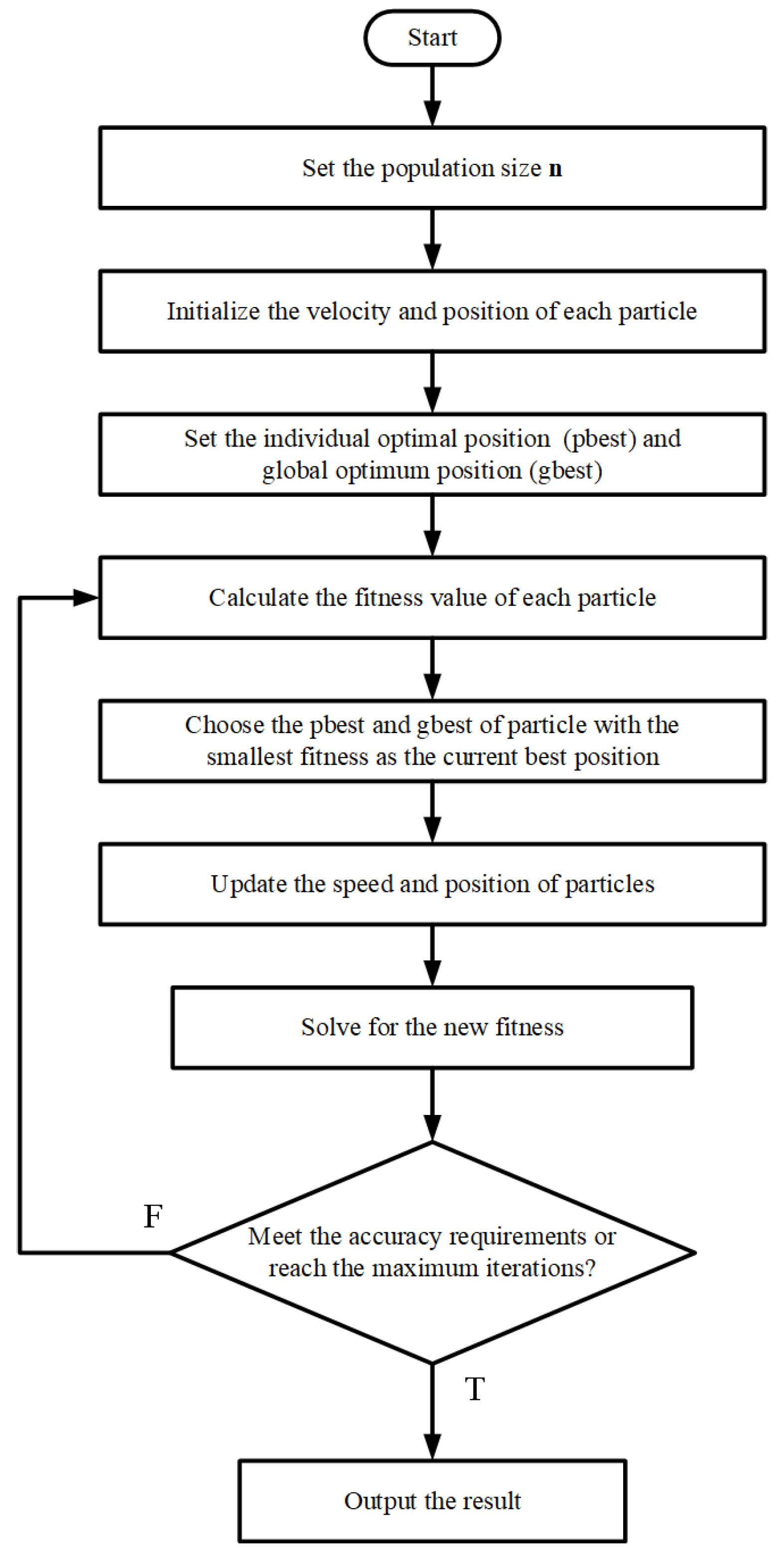
2.2. Particle Swarm Optimization Algorithm

In existing energy forecasting research, scholars mostly use heuristic algorithms to solve model parameters, including the genetic algorithm (GA) [33,34], ant colony algorithm (ACO) [35,36], gray wolf algorithm (GWO) [37,38], particle swarm optimization (PSO) [39,40], sparrow search algorithm (SSA) [41,42]. The parameters that need to be input, $\mathsf{\gamma },$ in the parameter selection process of the SVR model include the $\mathsf{\gamma }$ value and penalty factor, C. A simple grid search does not cover the parameter search space sufficiently and is prone to fall into local optimality, which leads to reduced training result accuracy [43]. Overly complex improved algorithms cannot filter out the noise in the data well and have the risk of overfitting [44]. The particle swarm optimization has the advantages of simplicity, strong adaptability, and strong global search ability. After comparing GA-SVR, GWO-SVR, and PSO-SVR, PSO-SVR demonstrated the best performance, as detailed in Section 3.3.2 Therefore, this paper selects the PSO for optimization.

Particle swarm optimization was proposed by Kennedy and Eberhart in 1995 based on the foraging behavior of bird flocks [45]. In the bird-flock foraging model, each individual is regarded as a particle, and the bird flock is regarded as a particle swarm. Finding the optimal solution to the problem is performed by simulating the movement and information exchange of particles in the solution space [46]. The basic idea is to continuously adjust the speed and position of particles to move them in a direction with better objective function values and to continuously optimize the search space through learning and communication. The algorithm evaluates the current position of each particle and updates the global optimal position to find the optimal fitness value. Its updates include particle velocity and position updates [47,48]. The particle speed update formula is shown in Equation (9).

$${\mathrm{v}}_{\mathrm{i}\mathrm{j}}^{\mathrm{t}+1}=\mathsf{\omega }{\mathrm{v}}_{\mathrm{i}\mathrm{j}}^{\mathrm{t}}+{\mathrm{c}}_1{\mathrm{r}}_{1\mathrm{j}}({\mathrm{p}\mathrm{b}\mathrm{e}\mathrm{s}\mathrm{t}}_{\mathrm{i}\mathrm{j}}-{\mathrm{x}}_{\mathrm{i}\mathrm{j}}^{\mathrm{t}})+{\mathrm{c}}_2{\mathrm{r}}_{2\mathrm{j}}({\mathrm{g}\mathrm{b}\mathrm{e}\mathrm{s}\mathrm{t}}_{\mathrm{j}}-{\mathrm{x}}_{\mathrm{i}\mathrm{j}}^{\mathrm{t}})$$

(9)

where ${\mathrm{v}}_{\mathrm{i}\mathrm{j}}^{\mathrm{t}+1}$ denotes the i updated value of the particle’s speed in the j dimension; $\mathsf{\omega }$ is the inertial weight, which controls the particle to maintain the original direction of movement; ${\mathrm{c}}_1$ and ${\mathrm{c}}_2$ are the acceleration factor; ${\mathrm{r}}_{1\mathrm{j}}$ and ${\mathrm{r}}_{2\mathrm{j}}$ are random numbers; ${\mathrm{p}\mathrm{b}\mathrm{e}\mathrm{s}\mathrm{t}}_{\mathrm{i}\mathrm{j}}$ is the individual optimal solution of the particle in the dimension; ${\mathrm{g}\mathrm{b}\mathrm{e}\mathrm{s}\mathrm{t}}_{\mathrm{j}}$ is the global optimal solution; and ${\mathrm{x}}_{\mathrm{i}\mathrm{j}}^{\mathrm{t}+1}$ is the current position of particle i in dimension j. The particle position update formula is shown in Equation (10).

$${\mathrm{x}}_{\mathrm{i}\mathrm{j}}^{\mathrm{t}+1}={\mathrm{x}}_{\mathrm{i}\mathrm{j}}^{\mathrm{t}}+{\mathrm{v}}_{\mathrm{i}\mathrm{j}}^{\mathrm{t}+1}$$

(10)

where ${\mathrm{x}}_{\mathrm{i}\mathrm{j}}^{\mathrm{t}+1}$ denotes the i updated value of the particle’s velocity in dimension j. After updating the position of each particle, it calculates the current fitness function value and updates the individual historical optimal position and the global historical optimal position until the maximum number of iterations is reached or the accuracy requirement is met. Output the solution corresponding to the global optimal position. Finally, optimal C (pbest) and optimal $\mathsf{\gamma }$ (gbest) are introduced into the model for model prediction and analysis. PSO can obtain the global optimal solution efficiently and quickly in the face of complex high-dimensional parameter spaces, and its performance is better, thereby achieving the effective optimization of support vector regression parameters.

2.3. PSO-SVR Model for Carbon Emissions Prediction

The carbon emissions of China’s logistics industry is studied in this paper. particle swarm optimization is used to optimize the parameters of the SVR model, for brevity, it is called as PSO-SVR model.

According to the characteristics of the particle swarm optimization algorithm, it includes the parameter settings of ${\mathrm{c}}_1,{\mathrm{c}}_2,\mathrm{n},\mathrm{k}$. Based on extensive literature reviews, ${\mathrm{c}}_1,{\mathrm{c}}_2$ denote the weights of the particle’s next segment of displacement originating from its own and the population’s experience. To avoid allowing the particle fall into a locally optimal solution and to improve its convergence speed, the value typically ranges between 1 and 2. Let ${\mathrm{c}}_1$ = 1.5, ${\mathrm{c}}_2$ = 1.7 [49], the number of populations be $\mathrm{N}$ = 50, and the maximum number of iterations be ${\mathrm{t}}_{\mathrm{m}\mathrm{a}\mathrm{x}}=150$. The inertia weight, $\mathrm{k}$, represents the displacement influence of the previous generation of particles on the current generation of particles. The larger the inertia weight, the greater the ability of the particles to explore the new region, and the greater the ability to search for the global optimal solution, but the corresponding ability to search for the local optimal solution will be weakened. The value typically ranges between 0.4 and 0.9 [50]. The model uses the dynamic adjustment of $\mathrm{k}$ in the search process to balance the abilities of the global search and local search as shown in Equation (11) below.

$$\mathrm{k}={\mathrm{k}}_{\mathrm{m}\mathrm{a}\mathrm{x}}-\left({\mathrm{k}}_{\mathrm{m}\mathrm{a}\mathrm{x}}-{\mathrm{k}}_{\mathrm{m}\mathrm{i}\mathrm{n}}\right)\times \frac{\mathrm{t}}{{\mathrm{t}}_{\mathrm{m}\mathrm{a}\mathrm{x}}}$$

(11)

where $\mathrm{t}$, ${\mathrm{t}}_{\mathrm{m}\mathrm{a}\mathrm{x}}$,${\mathrm{k}}_{\mathrm{m}\mathrm{i}\mathrm{n}}$, and ${\mathrm{k}}_{\mathrm{m}\mathrm{a}\mathrm{x}}$ represent the current iteration number, the maximum number of iterations, the minimum inertia weight, and the maximum inertia weight, respectively. The initial value of k is 0.6. Figure 1 shows the flow chart of the PSO algorithm.

3. Case Study

Initially, the carbon emissions values of China’s logistics industry for the period 2000–2021 are calculated in Section 3.1, and gray correlation analysis is applied to determine the factors influencing the carbon emissions data in Section 3.2. Finally, the model is formulated in Section 3.3.

3.1. Data Sources

Relevant energy consumption data for China’s logistics industry from 2000 to 2021, as well as the data of 12 influencing factors in the corresponding years, were used as the data set for this study (data from the website of China’s National Bureau of Statistics). Since the fuels used in the logistics industry are generally relatively carbon-intensive, their carbon emissions mainly come from energy consumption in various transportation, warehousing, and packaging stages. More than 80% comes from emissions caused by primary energy consumption, including coal, gasoline, natural gas, ${\mathrm{C}\mathrm{O}}_2$, etc. Therefore, this study uses the energy coefficient estimation method to estimate the carbon emissions data of the logistics industry. The equation is as follows.

$$\mathrm{C}=\sum _{\mathrm{i}=1}^{\mathrm{n}}{\mathrm{C}}_{\mathrm{i}}=\sum _{\mathrm{i}=1}^{\mathrm{n}}{\mathsf{\alpha }}_{\mathrm{i}}{\mathsf{\beta }}_{\mathrm{i}}{\mathsf{ϵ}}_{\mathrm{i}}$$

(12)

where $\mathrm{C}$ is the total carbon emissions from the logistics industry, ${\mathrm{C}}_{\mathrm{i}}$ is i the carbon emissions from energy, ${\mathsf{\alpha }}_{\mathrm{i}}$ is i the carbon emissions coefficient for energy, ${\mathsf{\beta }}_{\mathrm{i}}$ represents i, the standard coal conversion coefficient of energy, and ${\mathsf{ϵ}}_{\mathrm{i}}$ is the i consumption of energy. The specific coefficients of each energy source are from the “National Greenhouse Gas Emission Inventory Guidelines”, as shown in

Table 1. Table of energy coefficients.

Energy	Coal	Coke	Crude	Gasoline	Kerosene	Diesel Fuel	Fuel Oil	Natural Gas	Electricity
Standard Coal Conversion Coefficient	0.7143	0.9714	1.4286	1.4714	1.4714	1.4571	1.4286	1.3300	0.1229
Carbon Emissions Coefficient	0.7476	0.1128	0.5854	0.5532	0.3416	0.5913	0.6176	0.4479	2.213

.

The carbon emissions from the logistics industry are the key for achieving the “Dual Carbon” goal. Carbon emissions from the logistics industry have increased year by year. In 2020, they declined due to the impact of the COVID-19 pandemic. After 2021, when the economy gradually recovered, carbon emissions increased significantly. Their growth rate has become less volatile, also increasing from a negative growth to 7.5% in 2021. This further illustrates the indispensable position of the logistics industry in daily economic life, and the measurement of carbon emissions in the logistics industry will be of great significance to the achievement of the country’s “Dual Carbon” goals.

According to the calculation results of Formula (11), the trend of carbon emissions data in the logistics industry is shown in Figure 2.

3.2. Selection of Influencing Factors

As an environmental impact model, the STIRPAT model is an extension and improvement of the IPAT model. By adding external variables, including economic factors, population factors, energy structure, technological level, etc. [51], it better captures the impact of human activities on the environment and can more accurately predict environmental change. The formula is shown in Equation (12).

$$\mathrm{I}=\mathsf{\alpha }{\mathrm{P}}^{\mathrm{b}}{\mathrm{A}}^{\mathrm{c}}{\mathrm{T}}^{\mathrm{d}}\mathrm{E}$$

(13)

where I is the environmental pressure, a is the model coefficient; b, c, and d are the elastic coefficients of population, economy, and technical level, respectively; P is the population factor; A is the economic factor; T is the technical level; and E represents resource utilization efficiency.

Based on the definition of influencing factors by the STIRPAT model, this paper preliminarily selects 12 factors, including gross domestic product, gross logistics industry output, total social fixed-asset investment in the logistics industry, total import and export trade, actual foreign investment in the logistics industry, residents’ consumption level (absolute number), population size, proportion of urban population in the country, number of people employed in the tertiary industry, forest coverage rate, total energy consumption, and number of scientific and technological achievements registered, as carbon emissions evaluation factors for China’s logistics industry [52,53]. The selected influencing factors are shown in

Table 2. Selection of influencing factors of carbon emissions in the logistics industry.

Factor Category	Identification	Specific Indicators
Economic Factors	${\mathrm{A}}_1$	Gross domestic product (GDP)
	${\mathrm{A}}_2$	Logistics gross product
	${\mathrm{A}}_3$	Total social fixed-asset investment in the logistics industry
	${\mathrm{A}}_4$	Total import and export trade
	${\mathrm{A}}_5$	Actual used amount of foreign capital
	${\mathrm{A}}_6$	Residents’ consumption level (absolute number)
Demographic Factors	${\mathrm{P}}_7$	Population size
	${\mathrm{P}}_8$	The proportion of the urban population
	${\mathrm{P}}_9$	Number of employees in the tertiary industry
Energy Factors	${\mathrm{E}}_{10}$	Forest cover rate
	${\mathrm{E}}_{11}$	Total energy consumption (standard coal)
Technical Factors	${\mathrm{T}}_{12}$	Tertiary-industry-employed population

.

Our study aims to improve the correlation between the carbon emissions from the logistics industry and the influencing factors and provide more accurate data support for subsequent model training. After using the STIRPAT model to select the influencing factors, the gray correlation analysis GRA model was further used for the initial screening of the influencing factors. Gray correlation analysis is suitable for feature selection in cases of small samples, high dimensions, and non-uniform distributions. It can better handle data with nonlinear relationships, and the results have certain flexibility and versatility [54]. The carbon emissions from China’s logistics industry are taken as the parent sequence, and the other influencing factors are input as the feature sequence. The resolution coefficient $\mathsf{\rho }$ was between 0 and 1 [55]. To reduce the complexity of the model and improve its interpretability of the model, set $\mathsf{\rho }$ = 0.75. After the data was averaged and dimensionless, the gray correlation analysis was performed.

Fixed-asset investments in the logistics industry, population size, GDP, residents’ consumption level, forest coverage rate, and carbon emissions in China’s logistics industry correlated less than 0.75 and were eliminated. The remaining factors had a strong correlation with carbon emissions in the logistics industry. The correlation of each influencing factor is arranged in descending order, as shown in

Table 3. Gray correlation analysis ranking results.

Influencing Factors	Identification	Correlation
Total Energy Consumption	${\mathrm{x}}_{11}$	0.903
Number of Technological Achievements Registered	${\mathrm{x}}_9$	0.820
Actual Used Amount of Foreign Capital	${\mathrm{x}}_5$	0.813
Total Import and Export Trade	${\mathrm{x}}_4$	0.802
Tertiary-Industry-Employed Population	${\mathrm{x}}_{12}$	0.789
The Proportion of Urban Population in China	${\mathrm{x}}_8$	0.779
Logistics Gross Product	${\mathrm{x}}_2$	0.764

.

Finally, this paper selected total energy consumption (${\mathrm{E}}_2)$, number of technological achievements registered (${\mathrm{T}}_1)$, actual used amount of foreign capital (${\mathrm{A}}_5)$, total import and export trade (${\mathrm{A}}_4)$, tertiary-industry-employed population (${\mathrm{P}}_3)$, proportion of urban population in China $\left({\mathrm{P}}_2\right)$, and logistics gross product (${\mathrm{A}}_2)$ as the inputs of the model-independent variables, and used the carbon emissions value of the logistics industry as the dependent variable to train the model. The “Outline of the 14th Five-Year Plan for National Economic and Social Development of the People’s Republic of China and the Long-Term Objectives for 2035” also emphasizes scientific and technological innovations, foreign trade, industrial system reform, urbanization, economic development, and other issues. This shows that the variables selected in this paper have a policy basis and theoretical significance.

3.3. Prediction of the Carbon Emissions Level of China’s Logistics Industry Based on the PSO-SVR Model

3.3.1. Prediction of Carbon Emissions Level of China’s Logistics Industry

The sample period of this study is 2000–2021. Through the cross-validation method, 16 years of annual data were selected as training sets, and 7 years of annual data were selected as test sets. As can be seen in Section 3.2, a total of 7 influencing factors were used as input values of the support vector machine prediction model, and carbon emissions were used as the model output value. After the data were averaged and dimensionless, cross-validation was used to enable the model to be trained and evaluated multiple times on a limited data set. To ensure the accuracy of the results, the predicted value of carbon emissions data should fall within a reasonable fluctuation range of historical data, so as to avoid the prediction results being too far away from reality.

The PSO algorithm was used to optimize the penalty coefficient, C, and kernel function width, $\mathsf{\gamma }$, in the SVR algorithm. The range of the two parameters was set to (0.1, 100) and (0.01, 10) [56]. The specific process is detailed in Section 2.3. The particles were iteratively adjusted based on their own experience and the experience of the optimal individual. The SVM regression model was trained with the training set data. After multiple iterations were converged, the optimal parameters C = 3.6261; $\mathsf{\gamma }$ = 0.1202 were finally obtained. The fitness value of the particle here was the mean square error between the predicted value and the actual value. The fitting curve is shown in Figure 3.

To better capture the features of the data set and thus accurately predict new data, the input parameters were C = 3.6261, $\mathsf{\gamma }$ = 0.1202, and then the trained SVR model was used for the test set prediction. The training and test sets were divided into data labeled 1 to 16 and 1 to 6, respectively. The sets were obtained with excellent fitting effects, while there were some errors in the training set, which indicates that the testing effect effectively removes noise and has better generalization. The model was used to predict the level of carbon emissions in China’s logistics industry, and the algorithm is specified in Section 2. The model training and testing graphs are shown in (a) and (b), respectively, in Figure 4.

The MAPE of the testing set is 0.82%. The prediction results are accurate and effectively predict the carbon emissions level of the logistics industry. Then, we used the model to predict the unpublished carbon emissions data for the logistics industry in 2022 and achieved the result of 178,429,500 tonnes. The test and prediction results of the model are shown in

Table 4. Results of the PSO-SVR model.

Number	Actual Value (10,000 Tons)	Prediction Value (10,000 Tons)	Relative Error
1	5177.19	5210.35	0.64%
2	7586.50	7566.99	0.26%
3	11,601.80	11,672.03	0.61%
4	15,185.33	14,817.34	2.42%
5	17,497.62	17,510.34	0.07%
6	18,243.89	18,072.51	0.94%
Prediction	—	17,842.95	—
MAPE			0.82%

.

3.3.2. Prediction Result Comparison

For small samples of carbon emissions-related data, traditional models use time-series analysis, gray prediction, and other methods to simply output time indicators and carbon emissions data, failing to consider the changes in relevant influencing variables and the environment. Support vector regression in machine learning is significantly better than other models.

To verify the prediction effect of the model proposed in this article, this section also uses gray GM(1,1), ARIMA(0,1,0), metabolism-based FGM(1,1), support vector regression (SVR), genetic algorithm-optimized support vector regression (GA-SVR), and gray wolf algorithm-optimized support vector regression (GWO-SVR) models to predict the carbon emissions from China’s logistics industry, where the metabolism-based FGM (1,1) fractal order is r = 0.25, the SVR parameter is C = 4, $\mathsf{\gamma }=0$.8, the GA-SVR parameter is C = 1.9033, $\mathsf{\gamma }=2$.1408, the GWO-SVR parameter is C = 2.9826, $\mathsf{\gamma }=0$.6979, and the prediction error are shown in

Table 5. Prediction error comparison table.

Model	GM(1,1)	FGM(1,1) (r = 0.25)	ARIMA (0,1,0)	SVR (C = 4, γ = 0.8)	GWO-SVR (C = 2.9826, γ = 0.6979)	GA-SVR (C = 1.9033, γ = 2.1408)	PSO-SVR (C = 3.6261, γ = 0.1202)
MAPE	9.47%	7.01%	3.83%	2.03%	1.16%	1.15%	0.82%

.

As shown in Table 5, GM(1,1) has the worst prediction effect, with an MAPE as high as 9.4%; ARIMA(0,1,0) predicts a reduced MAPE of 7.01%. Among the time-series prediction models, FGM(1,1) has the highest prediction accuracy, with an error of 3.83. As for the machine learning models, the SVR model is significantly better than the time-series prediction model, with an MAPE value of 2.03%. Then, the gray wolf algorithm, genetic algorithm and particle swarm algorithm are chosen to perform the parameter search for optimization on the SVR, with a significant reduction in the MAPE value, and the search for optimization significantly improves the prediction accuracy. It is finally found that the particle swarm algorithm has a significant effect on SVR optimization. SVR optimization has a significant effect and the map value is only 0.82%, indicating that, for this carbon emissions data set, the PSO algorithm effectively handles its noise values and special values, and can be relatively efficient in parameter optimization. Secondly, the SVR model has an excellent fitting effect on the small samples and nonlinear data model. This study better verifies the relevant factors of carbon emissions, reflecting the characteristics of carbon emissions data. It is of great significance for the prediction and analysis of carbon emissions values.

4. Results and Discussion

As a comprehensive industry, the logistics industry is closely connected to other industries, especially the manufacturing industry. Achieving the national “Dual Carbon” goal requires a joint response from all fields. Therefore, measuring and analyzing the carbon emissions level of the logistics industry is of great significance for my country to achieve low-carbon development and expand new productivity. This study uses the STIRPAT model to initially select the influencing factors of carbon emissions in the logistics industry and combines the gray correlation model to screen the influencing factors. The particle swarm optimization support vector machine (SVR) regression model is used to train and predict the data. After the comparison with a single model and other optimization algorithm models, the following conclusions are drawn:

(1)

The gray correlation analysis was conducted on 12 influencing factors that affected carbon emissions in the logistics industry, and seven significant variables were finally screened out. These variables include total energy consumption, the number of registered scientific and technological achievements, the actual amount of foreign capital used in the logistics industry, the total amount of import and export trade, the number of employees in the tertiary industry, the proportion of the national urban population, and total national energy consumption. Gray relational analysis adopts a nonlinear approach, which effectively reduces the dimensionality of the predictive input set and enhances the practicability of the model [57]. Based on these analyses, the government should prioritize optimizing energy structures, strengthening technological innovation [58], utilizing foreign capital rationally, promoting balanced trade development [59], adjusting industrial structures, optimizing urban population distribution [60,61], and enhancing regulatory and law enforcement efforts. These policy recommendations will contribute to reducing carbon emissions in the logistics industry and facilitate its transition toward a green and low-carbon development path.

(2)

The SVR regression model was optimized using the particle swarm optimization algorithm. The mean absolute percentage error (MAPE) was merely 0.82%, significantly outperforming traditional forecasting methods. This result demonstrates the effectiveness and accuracy of the model in predicting carbon emissions from complex systems. The model is capable of capturing the dynamic characteristics of carbon emissions in the logistics industry and effectively forecasting future carbon emissions trends. Based on the forecasting results of the PSO-SVR model, the carbon emissions from China’s logistics industry are expected to reach 178.4295 million tons in the next year.

(3)

Relying solely on energy coefficient estimation methods as a basis for prediction has significant limitations. This approach tends to be based on static or macro-level assumptions. The logistics industry involves multiple processes and factors, such as the choice of transportation modes, the length of transportation distances, differences in cargo types, and the efficiency of warehouse management, all of which have significant impacts on carbon emissions and place higher demands on data. Furthermore, with the continuous development of technology, new optimization techniques are emerging, which may include predictive models based on large models [62] and machine learning. These techniques can more flexibly adapt to industry changes and more accurately simulate and predict carbon emissions in the logistics industry. This paper also acknowledges the need for continuous learning and updating.

References

1. Ren, R.; Gao, G. Chinese Pathway and Construction of Ecological Perspectives in the Context of Dual Carbon Goals—Taking English Reports on “Dual Carbon” in China Daily and Xinhua News Agency as Examples. J. Univ. Sci. Technol. Beijing (Soc. Sci. Ed.) 2024, 40, 94–103. [Google Scholar]
2. He, D. “New Blueprint” for High-quality Development of Modern Logistics—Interpretation of “14th Five-Year Plan for Modern Logistics Development”. China Storage Transp. 2023, 3, 17–19. [Google Scholar]
3. Yao, X.; Zhang, H.; Wang, X. Which model is more efficient in carbon emission prediction research? A comparative study of deep learning models, machine learning models, and econometric models. Environ. Sci. Pollut. Res. Int. 2024, 31, 19500–19515. [Google Scholar] [CrossRef]
4. Yang, D.; Li, Y.; Tian, C. Research on the natural peak characteristics and peak prediction of carbon emissions in the transportation industry. Transp. Syst. Eng. Inf. 2024, 24, 34–44. [Google Scholar]
5. Ju, K.; Li, S.; Ma, Y. Decomposition of influencing factors and peak scenario prediction of carbon emissions in China’s water transport industry. Logist. Technol. 2024, 47, 89–93. [Google Scholar]
6. Zhu, W.; Cheng, Y. Analysis of influencing factors of carbon emissions in China’s construction industry and prediction of carbon peak carbon neutrality. J. Hebei Inst. Environ. Eng. 2024, 34, 1–7. [Google Scholar]
7. Wang, J.; Wei, J. Change characteristics and scenario simulation of building operation carbon emissions in Beijing under time series. J. Beijing Univ. Technol. 2022, 48, 220–229. [Google Scholar]
8. Cheng, M.; Liu, Y.; Li, J. A new modeling method of gray GM (1, N) model and its application to predicting China’s clean energy consumption. Commun. Stat.-Simul. Comput. 2023, 52, 3712–3723. [Google Scholar] [CrossRef]
9. Cheng, M.; Li, J.; Liu, Y.; Liu, B. Forecasting Clean Energy Consumption in China by 2025: Using Improved Gray Model GM (1, N). Sustainability 2020, 12, 698. [Google Scholar] [CrossRef]
10. Deng, W.; Xu, Z. Characteristics of agricultural carbon emissions and carbon peak analysis in Hunan Province. Chin. J. Eco-Agric. 2024, 32, 206–217. [Google Scholar]
11. Shu, F. Forecast of China’s corrugated paper production based on FGM (1,1). China Pap. Ind. 2023, 44, 6–9. [Google Scholar]
12. Chen, T.; Wang, M. Deep Learning-Based Carbon Emission Forecasting and Peak Carbon Pathways in China’s Logistics Industry. Sustainability 2024, 16, 1826. [Google Scholar] [CrossRef]
13. Zhang, X.; Wei, Z.; Chen, Z.; Han, Y. Research on industrial carbon emission prediction method based on LASSO-GWO-KELM. Environ. Eng. 2023, 41, 141–149. [Google Scholar]
14. Shao, C.; Ning, J. Construction and application of carbon emission prediction model for China’s textile and garment industry based on improved WOA-LSTM. J. Beijing Inst. Fash. Technol. (Nat. Sci. Ed.) 2023, 43, 73–81. [Google Scholar]
15. Jiao, L.; Liu, Y.; Wu, Y. Research on carbon emission prediction of transportation industry based on convolutional neural network. Railw. Transp. Econ. 2024, 1–9. [Google Scholar]
16. Zhang, G.; Wang, T.; Lou, Y. Analysis of China’s provincial carbon peak path based on LSTM neural network. Chin. Manag. Sci. 2024, 1–12. [Google Scholar]
17. Wei, B.; Liu, C.; Liu, J. Multi-factor carbon emissions trading price prediction based on Transformer-LSTM model. Price Mon. 2024, 1–13. [Google Scholar]
18. Weige, N.; Ou, A.; Huiming, D. A novel gray prediction model with a feedforward neural network based on a carbon emission dynamic evolution system and its application. Environ. Sci. Pollut. Res. Int. 2022, 30, 20704–20720. [Google Scholar]
19. Wang, Q.; Wang, J.; Zhu, C. Research on carbon emission prediction of the transportation industry integrating VMD and SSA-LSSVR. Environ. Eng. 2023, 41, 124–132. [Google Scholar]
20. Cortes, C.; Vapnik, V. Support-Vector Networks. Mach. Learn. 1995, 20, 273–297. [Google Scholar] [CrossRef]
21. Liu, B.; Fu, C.; Li, J. Research on prediction of CO2 emissions in China based on PCA-SVR model. Arid Land Resour. Environ. 2018, 32, 56–61. [Google Scholar]
22. Yu, S.; Zou, H.; Yu, F.; Fu, C.; Han, N. Application of Fuzzy Neural Network in Short-Term Load Forecasting of Power Systems. Smart Grid 2018, 46, 88–91+97. [Google Scholar]
23. Fu, Y.; Cai, L.; Zheng, G. Failure diagnosis of electro hydraulic servo valve based on SA-PSO-SVM. J. Mech. Sci. Technol. 2022, 36, 5971–5976. [Google Scholar] [CrossRef]
24. Peng, N.; Zhang, Y.; Wang, X.; Zhao, P. Research on Classification Method of Acoustic Emission Signals of Welding Cold Cracks Based on VMD Energy Entropy and GA-SVM. China Meas. Test 2024, 50, 47–53. [Google Scholar]
25. Ren, W.; Yang, X.; Feng, Y.; Yang, L.; Wei, J. Prediction of Slope Deformation Based on GNSS Monitoring Using SSA-SVR Model. Saf. Environ. Eng. 2024, 31, 160–169. [Google Scholar]
26. Ding, Y.; Zhang, Z.; Liu, H. Fault Detection of Transformer Resonance Overvoltage Based on Multi-source Feature Fusion. Electr. Eng. Econ. 2024, 162–164+167. [Google Scholar]
27. Fan, S.; Zhao, Z.; Guo, J. A Review of Data-Driven Methods for Transient Stability Assessment of Power Systems. Proc. CSEE 2024, 44, 3408–3429. [Google Scholar]
28. Singla, M.; Shukla, K.K. Robust statistics-based support vector machine and its variants: A survey. Neural Comput. Appl. 2020, 32, 11173–11194. [Google Scholar] [CrossRef]
29. Shu, H.; Wu, D.; Chen, C. Analysis of Airtightness Detection Method for the Main Brake Cylinder of Electric Vehicles. China Mach. 2023, 77–80. [Google Scholar]
30. Mu, S.; Shen, W.; Lv, D.; Song, W.; Tan, R. Research Progress on Electronic Nose Technology and Its Applications. Mater. Rep. 2024, 1–34. [Google Scholar]
31. Yang, Y.; Liu, J.; Chen, T.; Wei, W.; Wang, S. Short-term natural gas load forecasting based on the PSO-SVR model. Sci. Technol. Eng. 2023, 23, 15210–15216. [Google Scholar]
32. Liu, H.; Wang, L.; Wang, Y.; Xi, L. Wheat yield prediction method in Henan Province based on PSO-SVR model. J. Jiangsu Agric. Sci. 2023, 51, 157–163. [Google Scholar]
33. Zhou, Q.; Zhang, X.; Chen, J.; Shen, W.; Bai, J.; Huang, Y.; Tang, S. Photovoltaic power station power generation prediction method based on genetic algorithm wavelet neural network. Smart Electr. 2024, 52, 78–84. [Google Scholar]
34. Liu, Y.; Ding, S. Research on energy loss in green building design. Housing 2024, 104–107. [Google Scholar]
35. Bao, X.; Liu, S.; Zhang, N. Computing power flexible migration optimization algorithm based on improved ant colony algorithm. Electr. Power Inf. Commun. Technol. 2024, 22, 1–8. [Google Scholar]
36. Feng, L.; You, W. Short-term prediction technology of photovoltaic power generation based on ant colony algorithm. Commun. Inf. Technol. 2023, 36–39. [Google Scholar]
37. Chen, K.; Ding, M.; Liu, J.; Duan, J.; Liu, C.; Xu, D. Short-term wind power forecasting based on improved grey wolf algorithm to optimize WLSSVM. Inn. Mong. Electr. Power Technol. 2024, 42, 1–7. [Google Scholar]
38. Chen, P.; Zhou, J.; Wu, M. Research on online metering error prediction method for DC charging piles based on the improved GWO-GM(1,1) model. Mod. Electron. Technol. 2024, 47, 112–117. [Google Scholar]
39. Chen, Y.; Ma, X.; Cheng, K.; Bao, T.; Chen, Y.; Zhou, C. Ultra-short-term power prediction of new energy based on meteorological feature selection and SVM model parameter optimization. J. Sol. Energy 2023, 44, 568–576. [Google Scholar]
40. Liang, Z.; Zhou, Y.; Feng, D.; Guo, L.; Du, Y. Day-ahead optimal dispatch of the park’s comprehensive energy system considering the coupling of the electricity carbon green certificate market. Electr. Power Constr. 2023, 44, 43–53. [Google Scholar]
41. Yao, H.; Li, C.; Yang, P. Building cooling capacity prediction based on the Sine-SSA-BP algorithm. Comput. Simul. 2023, 40, 525–529+540. [Google Scholar]
42. Xie, S.; He, S.; Yan, X.; Zhang, Q. Photovoltaic short-term power prediction based on SSA-BP neural network. J. Zhejiang Univ. Technol. 2022, 50, 628–633. [Google Scholar]
43. Yang, Y.; Li, L.; Lin, H. Parameter Parallelization: A Machine Learning Parameter Optimization Method Based on Swarm Heuristic Algorithm. Sci. Technol. Eng. 2022, 22, 1972–1980. [Google Scholar]
44. Ni, D. Research on Corporate Credit Risk Prediction Based on High-Dimensional Small Sample Data. Ph.D. Thesis, Chongqing University, Chongqing, China, 2021; pp. 127–130. [Google Scholar]
45. Kennedy, J.; Eberhart, R. Particle Swarm Optimization. In Proceedings of the International Conference on Neural Networks, Perth, Australia, 27 November–1 December 1995. [Google Scholar]
46. Eberhart, R.C.; Kennedy, J. A New Optimizer Using Particle Swarm Theory. In Proceedings of the 6th International Symposium on Micro Machine and Human Science, Nagoya, Japan, 4–6 October 1995. [Google Scholar]
47. Zou, H.; Song, J.; Liu, Y.; Duan, Z.; Zhang, X.; Song, L. Transmission Line Ice-Coating Galloping Prediction Model Based on PSO-SVM Algorithm. J. Vib. Shock 2023, 42, 280–286. [Google Scholar]
48. Zhao, S.; Zhao, Z. A comparative study of landslide susceptibility mapping using SVR and PSO-SVR models based on grid and slope units. Math. Probl. Eng. 2021, 2021, 8854606. [Google Scholar]
49. Zeng, Q.; Chen, G.; Li, W.; Meng, J.; Li, G.; Tong, J.; Tian, Z.; Zhang, X.; Li, G.; Guo, L.; et al. Rapid Detection and Classification of Steel Based on Particle Swarm Optimization-Support Vector Machine Algorithm Using Laser-Induced Breakdown Spectroscopy. Spectrosc. Spectr. Anal. 2024, 44, 1559–1565. [Google Scholar]
50. Xu, H.; Tian, C.; Mao, R.; Gu, X.; Chang, C. Research on the Prediction Model of Air Material Consumption Based on PSO-SVM. Mod. Inf. Sci. Technol. 2024, 8, 142–145. [Google Scholar]
51. Wang, K.; Niu, D.; Zhen, H.; Sun, L.; Xu, X. Research on China’s carbon emissions prediction based on the WOA-ELM model. Ecol. Econ. 2020, 36, 20–27. [Google Scholar]
52. Wang, Y.; Li, Y.; Wang, H.; Dong, P.; Teng, Y.; Lin, Y.; Liu, L. Prediction of Carbon Emissions in Hebei Province Based on an Improved BP Neural Network. Ecol. Econ. 2024, 40, 30–37. [Google Scholar]
53. Li, G.; Huang, Q. Scenario Prediction of Carbon Peak in Beijing-Tianjin-Hebei Region Based on Lasso-GRNN Neural Network Model. Environ. Sci. 2024, 1–21. [Google Scholar]
54. Feng, M.; Zhou, D.; Yang, Y. SWOT Analysis and Countermeasure of Jilin Province Aviation Logistics Industry Development Strategy Based on Low Carbon and Environmental Protection. IOP Conf. Ser. Earth Environ. Sci. 2019, 252, 042043. [Google Scholar] [CrossRef]
55. Shen, Y.; Liu, C. Mining of Users’ Key Needs Based on Opinion Leaders in Online Brand Communities. Comput. Technol. Dev. 2024, 34, 23–31. [Google Scholar]
56. Li, Y.; Wang, Y. Urban rail transit section passenger flow prediction based on PSO-LSSVM algorithm. J. Chang. Univ. (Nat. Sci. Ed.) 2021, 41, 91–102. [Google Scholar]
57. Hu, S.; Wang, P.; Zhao, X.; Zhang, G. Feature Extraction of Decision-Making Parameters in Spinning Production Process Based on Equidistant Feature Mapping. J. Mach. Des. 2024, 41, 82–90. [Google Scholar]
58. Ma, Y.; Li, Y.; Ma, L. Spatial Correlation Effects and Influencing Factors of Green and Low-Carbon Development in China’s Logistics Industry. Environ. Sci. 2024, 1–13. [Google Scholar]
59. The People’s Government of Jiangsu Province. Several Opinions of the CPC Jiangsu Provincial Committee and the Jiangsu Provincial People’s Government on Deeply Implementing the Strategy of Economic Internationalization and Comprehensively Improving the Development Level of an Open Economy. Bull. Jiangsu Prov. People’s Gov. 2012, 5–13.
60. Zhu, X. Research on Evaluation and Prediction of High-Quality Development of China’s Logistics Industry. Master’s Thesis, Beijing University of Posts and Telecommunications, Beijing, China, 2021. [Google Scholar]
61. Wang, L.; Chen, Z. Research on the Efficiency of China’s Logistics Industry under Energy and Environmental Constraints; Nankai University Press: Tianjin, China, 2020; 141p. [Google Scholar]
62. Wei, X.; Feng, X.; Jiang, H. Research on Carbon Emission Prediction Based on Multi-head Attention CNN-LSTM. J. Chongqing Technol. Bus. Univ. (Nat. Sci. Ed.) 2024, 1–11. [Google Scholar]
Figure 1. Flow chart of the particle swarm optimization algorithm.
Mathematics 12 01980 g001
Figure 2. Carbon emissions trend of China’s logistics industry from 2000 to 2021.
Mathematics 12 01980 g002
Figure 3. PSO-optimized SVR fitness curve.
Mathematics 12 01980 g003
Figure 4. Comparison of (a) training results with actual values, (b) testing results with actual values.
Mathematics 12 01980 g004