Exponential Synchronization of Coupled Neural Networks with Hybrid Delays and Stochastic Distributed Delayed Impulses

Abstract

This paper is concerned with exponential synchronization for a class of coupled neural networks with hybrid delays and stochastic distributed delayed impulses. First of all, based on the average impulsive interval method, total probability formula and ergodic theory, several novel impulsive Halanay differential inequalities are established. Two types of stochastic impulses, i.e., stochastic distributed delayed impulses with dependent property and Markov property have been taken into account, respectively. Secondly, some criteria on exponential synchronization in the mean square of a class of coupled neural networks with stochastic distributed delayed impulses are acquired by combining the proposed lemmas and graph theory. The validity of the theoretical results is demonstrated by several numerical simulation examples.

1. Introduction

In recent years, the dynamical properties of neural networks (NNs) have been extensively investigated due to NNs’ high-nonlinearity and good fault tolerance. Various kinds of NNs including Hopfield NNs, Cohen-Grossber NNs, BAM NNs and inertial NNs have been proposed and examined. Moreover, coupled neural networks (CNNs) can be regarded as one kind of complicated NN composed of multiple interconnected nodes. In contrast to NNs with single nodes, CNNs possess more elaborate and unforeseeable characteristics. Recently, a considerable number of results with respect to the collective behavior of CNNs have been reported [1,2,3,4].

Synchronization is an interesting and important class of collective behavior and depicts that several systems adapt each other to a common trajectory that may be an equilibrium point, periodic solution, or chaotic attractor. Since Pecora and Carroll [5] introduced the synchronization of two identical chaotic systems, the synchronization issue has gained considerable attention because it can describe many natural phenomena and has many potential applications for image processing, secure communication, and neuronal synchronization. For instance, the theta rhythm related to the behavior of animals is produced by partial synchronization of neuronal activity in the hippocampal network, and an excessive synchronization of the neuronal activity over a wide area in the brain results in the epileptic rhythm [6]. Currently, various approaches to synchronization of CNNs have been developed including pinning control [7], adaptive control [8], event-triggered control [9], sampling control [10], periodic intermittent control [11], sliding control [12], impulsive control [13,14] and so on. Particularly, in [8], several criteria on exponential synchronization in the mean square and the almost sure sense for a class of neutral stochastic CNNs have been provided by combining M-matrix theory and algebraic inequalities, and adaptive controllers have been designed. In the real environment, it is desirable to realize synchronization within a finite horizon. Consequently, finite-time and fixed-time synchronization [15] of CNNs have been examined which exhibit strong robustness and anti-interference capability.

In addition, some practical networks such as electronic networks and biological networks frequently encounter momentary disturbances and abrupt variations, which could be characterized as impulses. Generally, impulses can be categorized into stabilizing impulses, destabilizing impulses and hybrid impulses. Numerous achievements relevant to the dynamic behaviors of CNNs with impulsive effects have been published. For instance, asymptotic synchronization of CNNs with time delays and stabilizing impulses has been studied by utilizing the stability theory for impulsive functional differential equations in [16] while exponential synchronization issue of CNNs has been dealt with through destabilizing impulses in [17]. By referring to [16,17,18], unified synchronization criteria in an array of CNNs with hybrid impulses have been established, and several concepts on average impulsive interval and average impulsive gain have been put forward in [19]. Furthermore, by using the improved Razumikhin approach, several criteria on pth moment exponential stability of non-autonomous stochastic delayed systems with impulsive effects have been derived in [20,21]. Actually, time delays also exist at the moment of the impulses and affect the dynamic properties in some applicable systems including signal transmission processing and biology systems. Numerous studies about stability and synchronization of nonlinear systems with delayed impulses have been carried out [22,23,24,25]. In [22], by utilizing the impulsive control theory and some comparison principles, various stability of nonlinear systems with state-dependent impulses have been examined. In [25], in light of the average impulsive delay–gain approach, exponential synchronization of CNNs with hybrid delayed impulses has been analyzed. The aforementioned impulsive delays are constant delays or time-varying delays, and one new class of distributed-delay-dependent impulses [26,27,28,29,30,31] has also caught the researchers’ attention. In [28,29], several impulsive Halanay differential inequalities have been presented and applied to the synchronization of network systems with distributed delayed impulses. Furthermore, the mean square stability of stochastic functional systems with distributed delayed impulses has been discussed based on the stochastic analysis technique and average dwell time method in [30,31]. Due to the existence of stochastic disturbances at the impulsive moment, stochastic impulses [32,33,34,35,36,37,38] have been introduced. In [34], under the circumstance that the impulse intensities were supposed to be random, the exponential synchronization problem of the neural networks (NNs) has been tackled, and the results have been further generalized to inertial network systems with stochastic delayed impulses [35,36].

It can be seen that the existing achievements in [26,27,28,29,30,31] are related to the deterministic distributed delayed impulses. Particularly, in [27], exponential synchronization of chaotic NNs with distributed delayed impulses has been examined, and the theoretical work has been extended to CNNs with time-varying delays of unknown bounded in [28]. However, so far, the synchronization issue of CNNs with hybrid delays and stochastic distributed delayed impulses has not been explored. Actually, when some factors such as hybrid delays and stochastic distributed delayed impulses are taken into account simultaneously, the approaches in [34,35,36] can not be directly applied to this case. How to overcome the difficulties that these factors bring is full of challenges. Additionally, the parameter c is limited to the condition $0<c\le 1$ in [34] and $c=1$ in [35], and impulses can not have a positive impact on the synchronization realization of coupled inertial NNs with hybrid delays in [36]. Consequently, how to relax these constraints and reduce the conservativeness of the existing work [34,35,36] is of great significance.

Inspired by the above discussions, we aim to explore the exponential synchronization of a class of CNNs with hybrid delays and stochastic distributed delayed impulses. To begin with, we propose two novel impulsive Halanay differential inequalities, where two types of stochastic impulses, i.e., stochastic distributed delayed impulses with dependent property and Markov property have been considered, respectively. Furthermore, combining the proposed lemmas and graph theory, some criteria on exponential synchronization in the mean square of a class of CNNs with stochastic distributed delayed impulses are obtained. The main contributions can be unfolded in three aspects.

(1)

Different from the deterministic distributed delayed impulses in the literature [26,27,28,29,30,31], in this paper, the intensities of distributed delayed impulses are supposed to be random. Two types of stochastic impulses including stochastic distributed delayed impulses with independent property and Markov property have been explored, respectively.

(2)

Based on the average impulsive interval method, total probability formula and ergodic theory, two novel impulsive Halanay differential inequalities are established, which generalize the findings in the literature [34,35] since time-varying delays, distributed delays and stochastic distributed delayed impulses are introduced simultaneously. Parameter c can be arbitrarily chosen. In view of invariant distribution theory, the stochastic impulses with Markov property are tackled.

(3)

By utilizing the established inequalities and graph theory, some criteria for exponential synchronization of CNNs with stochastic distributed delayed impulses are derived. In [36], impulses can only be regarded as outer disturbances for coupled inertial NNs with hybrid delays. Compared with the work [36], in this paper, impulses may also be viewed as outer perturbations or stabilizing sources, and the case of stochastic impulses with Markov property is also discussed.

The remainder of this paper is arranged as follows. In Section 2, some necessary definitions and assumptions are given, and two novel impulsive Halanay differential inequalities are established. In Section 3, a class of coupled neural networks with stochastic distributed delayed impulses is presented and several criteria on exponential mean square synchronization are derived. In Section 4, two numerical simulation examples are provided to show the validity of the theoretical results. Conclusions are drawn in the last section.

Notations: Let $\mathbb{R}$ and ${\mathbb{R}}^{+}$ be the set of real numbers and the set of non-negative real numbers, respectively. ${\mathbb{N}}^{+}$ stands for the set of positive integer numbers. $C({\mathbb{R}}^{+},\mathbb{R})$ denotes the set of continuous functions $v:{\mathbb{R}}^{+}\to \mathbb{R}$. $D^{+}v(t)$ represents the upper right Dini derivative of a function $v(t)$. $B={(b_{ij})}_{m\times n}$ denotes an $m\times n$ matrix, and $B^T$ denotes the transpose of matrix B. ${\lambda }_{\max }(B)$ denotes the maximal eigenvalue. For a random variable $\beta$, $E(\beta )$ and $D(\beta )$ denote the mathematical expectation and the variance, respectively. $\beta \sim U(a,b)$ and $\beta \sim E(c)$ indicate that $\beta$ obeys the uniform distribution and the exponential distribution, respectively. $P(A)$ represents the probability of the random event A.

2. Preliminaries

In this section, we will propose some necessary definitions and assumptions. Meanwhile, based on the average impulsive interval method, total probability formula and ergodic theory, two novel impulsive Halanay differential inequalities with hybrid delays are given. Two types of stochastic impulses, i.e., stochastic distributed delayed impulses with dependent property and Markov property have been taken into account, respectively.

Definition 1.

Suppose that $\Theta =\{t_1,t_2,\cdots ,t_n\}$ is the impulsive sequence and $T_a$ is the average impulsive interval. If $T_a\in {\mathbb{R}}^{+},N_0\in {\mathbb{N}}^{+}$ satisfied

$$\frac{T-t}{T_a}-N_0\le N_{\Theta }(T,t)\le \frac{T-t}{T_a}+N_0,\forall T\ge t\ge 0,$$

(1)

let $N_{\Theta }(T,t)$ be the number of impulsive times and Θ be the impulsive sequence on the interval $[t,T]$.

Assumption 1.

Let ${\left\{{\beta }_k\right\}}_{k=1,2,\dots }$ denote a sequence of independent and identically distributed random variables satisfying

$$\left\{\begin{array}{cc}\hfill E{\beta }_k=& \alpha >0,\hfill \\ \hfill D{\beta }_k\le & {\gamma }^2,\hfill \\ \hfill {\beta }_k\ge & 0,\hfill \end{array}\right.$$

(2)

where γ is a determined non-negative constant.

Lemma 1.

Let $\Theta =\{t_1,t_2,\cdots ,t_n\}$ denote the impulsive sequence and $T_a$ denote the average impulsive interval. Suppose that Assumption 1 holds. Function $v(t)\in C({\mathbb{R}}^{+},\mathbb{R})$, $t\ge t_0(t\ne t_k)$ satisfies the following differential inequality with stochastic distributed delayed impulses

$$\left\{\begin{array}{cc}\hfill D^{+}v(t)\le & -pv(t)+qv(t-{\sigma }_1(t))+r{\int }_{t-{\sigma }_2}^{t}v(s)ds,t\ne t_k,\hfill \\ \hfill v(t_k)\le & {\beta }_k{\int }_{t-{\rho }_k}^{t}v(s)ds,t=t_k,k=1,2,\cdots ,\hfill \\ \hfill v(t)=& \Phi (t),t\in [t_0-{\tau }_0,t_0],\hfill \end{array}\right.$$

(3)

where $v(t_k)=v(t_k^{+})$, $0\le {\rho }_k\le \rho$, ${\sigma }_2\ge {\rho }_k$, ${\sigma }_1(t)\le {\sigma }_1$, ${\tau }_0=\max \{{\sigma }_1,{\sigma }_2\}$, $p\ge 0$, $q\ge 0$, $r\ge 0$ and ${\parallel {\Phi }_{t_0}\parallel }_{{\tau }_0}=\underset{-{\tau }_0\le s\le 0}{\sup }\parallel \Phi (t_0+s)\parallel$. Denote $M_1=\max \left\{c^{-\frac{{\sigma }_1}{T_a}-N_0},1\right\}$ and $M_2=\max \left\{c^{-\frac{{\sigma }_2}{T_a}-N_0},1\right\}$. If $p>q{M}_1+r{M}_2{\sigma }_2\ge 0$, then we have

$$\begin{array}{c}\hfill Ev(t)\le M_0{\parallel {\Phi }_{t_0}\parallel }_{{\tau }_0}{e}^{-\left({\displaystyle \overline{ϵ}}-\frac{\ln \lambda }{T_a}\right)(t-t_0)},\forall t\ge t_0,\end{array}$$

(4)

where $\lambda \triangleq \min \left\{\alpha {\rho }_i{e}^{{\displaystyle \overline{ϵ}}{\rho }_i}+\frac{c{\rho }_i^2{e}^{2{\displaystyle \overline{ϵ}}{\rho }_i}{\gamma }^2}{{(\alpha {\rho }_i{e}^{{\displaystyle \overline{ϵ}}{\rho }_i}-c)}^2},\alpha {\rho }_i{e}^{{\displaystyle \overline{ϵ}}{\rho }_i}+c\right\}$, $M_0\triangleq \max \{{\lambda }^{-N_0},{\lambda }^{N_0}\}$, $c\ne \alpha {\rho }_i{e}^{{\displaystyle \overline{ϵ}}{\rho }_i}$ and ${\displaystyle \overline{ϵ}}>0$ is the unique solution of $\Pi (ϵ)=ϵ-p+q{M}_1{e}^{{\sigma }_1ϵ}+r{M}_2\frac{1}{ϵ}(e^{{\sigma }_2ϵ}-1)=0$.

Proof. 

Construct the following function

$$\begin{array}{c}\hfill \Pi (ϵ)=ϵ-p+q{M}_1{e}^{ϵ{\sigma }_1}+r{M}_2\frac{1}{ϵ}(e^{ϵ{\sigma }_2}-1).\end{array}$$

(5)

Noting that $\underset{ϵ\to 0^{+}}{\lim }\Pi (ϵ)=-p+q{M}_1+r{M}_2{\sigma }_2<0$, $\underset{ϵ\to +\infty }{\lim }\Pi (ϵ)>0$ and ${\Pi }^{\prime }(ϵ)>0$, there exists a unique positive root ${\displaystyle \overline{ϵ}}$ for equation $\Pi (ϵ)=0$. Subsequently, we will claim that

$$v(t)\le \left(\prod _{i=1}^k{\mu }_i\right){\parallel {\Phi }_{t_0}\parallel }_{{\tau }_0}{e}^{-{\displaystyle \overline{ϵ}}(t-t_0)},t\in [t_k,t_{k+1}),k=0,1,2,\dots ,$$

(6)

where ${\mu }_i\triangleq \max \{{\beta }_i{\rho }_i{e}^{{\displaystyle \overline{ϵ}}{\rho }_i},c\},i=1,2,\dots ,$ and $c>0$. When $t\in [t_0-\tau ,t_0]$, obviously, $v(t)\le {\parallel {\Phi }_{t_0}\parallel }_{\tau }$. Let $\Gamma >{\parallel {\Phi }_{t_0}\parallel }_{{\tau }_0}$. In order to show that assertion (5) holds, we need to prove that

$$v(t)<\Gamma \left(\prod _{i=1}^k{\mu }_i\right)e^{-{\displaystyle \overline{ϵ}}(t-t_0)}=z_k(t),\forall t\in [t_k,t_{k+1}),k=0,1,2,\dots .$$

(7)

When $k=0$, since the system is not influenced by impulse, we need to show that

$$v(t)<\Gamma e^{-{\displaystyle \overline{ϵ}}(t-t_0)}\triangleq z_0(t),\forall t\in [t_0,t_1).$$

(8)

Assume that inequality (8) is not satisfied, there exists a $t^{*}\in [t_0,t_1)$ such that

$$\begin{array}{c}\hfill v(t)<\Gamma e^{-{\displaystyle \overline{ϵ}}(t-t_0)},t\in [t_0,t_{*}),v(t^{*})=\Gamma e^{-{\displaystyle \overline{ϵ}}(t^{*}-t_0)};D^{+}v(t^{*})\ge D^{+}{z}_0(t^{*}).\end{array}$$

(9)

It follows from (9) that

$$\begin{array}{cc}\hfill D^{+}v(t^{*})\le & -pv(t^{*})+qv(t^{*}-{\sigma }_1(t))+r{\int }_{t^{*}-{\sigma }_2}^{t^{*}}v(s)ds\hfill \\ \hfill <& -p\Gamma e^{-{\displaystyle \overline{ϵ}}(t^{*}-t_0)}+q\Gamma e^{-{\displaystyle \overline{ϵ}}(t^{*}-{\sigma }_1-t_0)}+r{\int }_{t*-{\sigma }_2}^{t*}\Gamma e^{-{\displaystyle \overline{ϵ}}(s-t_0)}ds\hfill \\ \hfill <& \left[-p+q{M}_1{e}^{{\sigma }_1{\displaystyle \overline{ϵ}}}+\frac{r}{{\displaystyle \overline{ϵ}}}(e^{{\sigma }_2{\displaystyle \overline{ϵ}}}-1)M_2\right]z_0(t^{*})\hfill \\ \hfill =& D^{+}{z}_0(t^{*}),\hfill \end{array}$$

(10)

which means that $D^{+}v(t^{*})<D^{+}z(t^{*})$. It yields a contradiction with (9). Hence, inequality (8) holds. Assume that inequality (7) holds for $k\le m_0-1,m_0\in {\mathbb{N}}^{+}$, i.e.,

$$v(t)<z_k(t),\forall t\in [t_k,t_{k+1}),k=1,2,\dots ,m_0-1.$$

(11)

In what follows, we need to prove that inequality (7) is true for $k=m_0$. Actually, when $t=t_{m_0}$, one has that $v(t_{m_0})<{\beta }_{m_0}{\int }_{t-{\rho }_{m_0}}^{t_{m_0}}\Gamma \left({\displaystyle \prod _{i=1}^{m_0-1}}{\mu }_i\right)e^{-{\displaystyle \overline{ϵ}}(s-t_0)}ds\le \Gamma {\beta }_{m_0}{e}^{{\displaystyle \overline{ϵ}}{\rho }_{m_0}}{\rho }_{m_0}\left({\displaystyle \prod _{i=1}^{m_0-1}}{\mu }_i\right)e^{-{\displaystyle \overline{ϵ}}(t_{m_0}-t_0)}\le \Gamma \left({\displaystyle \prod _{i=1}^{m_0}}{\mu }_i\right)e^{-{\displaystyle \overline{ϵ}}(t_{m_0}-t_0)}\le z_{m_0}(t_{m_0})$. If inequality (7) is incorrect for $t\in (t_{m_0},t_{m_0+1})$, then there exists a $t_{*}\in (t_{m_0},t_{m_0+1})$ such that

$$\begin{array}{c}\hfill v(t)<z_{m_0}(t),t\in [t_{m_0},t_{*}),v(t_{*})=z_{m_0}(t_{*});D^{+}v(t_{*})\ge D^{+}{z}_{m_0}(t_{*}).\end{array}$$

(12)

For $\forall t\in [t_{*}-{\sigma }_1,t_{*})$, suppose $t\in [t_{b_t},t_{b_t+1})$, where $b_t$ is related to t. It follows from inequalities (11) and (12)

$$\begin{array}{c}\hfill v(t)<z_{b_t}(t),\forall t\in [t_{*}-{\sigma }_1,t_{*}).\end{array}$$

(13)

Noting that ${\mu }_i\ge c$, we may know that

$$\begin{array}{c}\hfill v(t)<z_{b_t}(t)=\frac{1}{{\mu }_{b_t+1}\dots {\mu }_{m_0}}\left(\prod _{i=1}^{m_0}{\mu }_i\right)\Gamma e^{{\displaystyle \overline{ϵ}}(t_{*}-t)}{e}^{-{\displaystyle \overline{ϵ}}(t_{*}-t_0)}\le \frac{e^{{\displaystyle \overline{ϵ}}(t_{*}-t)}}{c^{m_0-b_t}}{z}_{m_0}(t_{*}),\forall t\in [t_{*}-{\sigma }_1,t_{*}).\end{array}$$

(14)

Let $t_{*}-{\sigma }_1\in [t_{d_0},t_{d_0+1})$; we can find that $b_t\in [d_0,m_0]$. According to Definition 1, we can derive that

$$\begin{array}{c}\hfill 0\le m_0-b_t\le m_0-d_0=N_{\Theta }(t_{*}-{\sigma }_1,t_{*})\le \frac{{\sigma }_1}{T_a}+N_0,\forall t\in [t_{*}-{\sigma }_1,t_{*}).\end{array}$$

(15)

When $c\le 1$, combining inequalities (14) and (15) yields

$$v(t)<c^{-\frac{{\sigma }_1}{T_a}-N_0}{e}^{{\displaystyle \overline{ϵ}}(t_{*}-t)}{z}_{m_0}(t_{*}),\forall t\in [t_{*}-{\sigma }_1,t_{*}).$$

(16)

When $c>1$, according to inequalities (14) and (15), we obtain that

$$v(t)<e^{{\displaystyle \overline{ϵ}}(t_{*}-t)}{z}_{m_0}(t_{*}),\forall t\in [t_{*}-{\sigma }_1,t_{*}).$$

(17)

Since $z_{m_0}(t)$ is decreasing, it satisfies the following inequality

$$v(t_{*}-{\sigma }_1(t_{*}))<\max \left\{c^{-\frac{{\sigma }_1}{T_a}-N_0},1\right\}{e}^{{\sigma }_1{\displaystyle \overline{ϵ}}}{z}_{m_0}(t_{*})=M_1{e}^{{\sigma }_1{\displaystyle \overline{ϵ}}}{z}_{m_0}(t_{*}).$$

(18)

Similarly, when $s\in [t_{*}-{\sigma }_2,t_{*}]$, we also have that

$$v(s)<\max \left\{c^{-\frac{{\sigma }_2}{T_a}-N_0},1\right\}{e}^{{\displaystyle \overline{ϵ}}(t_{*}-s)}{z}_{m_0}(t_{*}).$$

(19)

It follows from inequality (18) and inequality (19) that

$$\begin{array}{cc}\hfill D^{+}v(t_{*})\le & -pv(t_{*})+qv(t_{*}-{\sigma }_1(t_{*}))+r{\int }_{t_{*}-{\sigma }_2}^{t_{*}}v(s)ds\hfill \\ \hfill <& -p{z}_{m_0}(t_{*})+q{M}_1{e}^{{\sigma }_1{\displaystyle \overline{ϵ}}}{z}_{m_0}(t_{*})+r\max \left\{c^{-\frac{{\sigma }_2}{T_a}-N_0},1\right\}{z}_{m_0}(t_{*}){\int }_{t_{*}-{\sigma }_2}^{t_{*}}{e}^{{\displaystyle \overline{ϵ}}(t_{*}-s)}ds\hfill \\ \hfill =& \left[-p+q{M}_1{e}^{{\displaystyle \overline{ϵ}}{\sigma }_1}+r{M}_2\frac{1}{{\displaystyle \overline{ϵ}}}(e^{{\displaystyle \overline{ϵ}}{\sigma }_2}-1)\right]z_{m_0}(t_{*})\hfill \\ \hfill =& D^{+}{z}_{m_0}(t_{*}),\hfill \end{array}$$

(20)

which means that $D^{+}v(t_{*})<D^{+}z(t_{*})$. It yields a contradiction with inequality (12). Hence, inequality (7) is true when $k=m_0$. Let $\Gamma \to {\parallel {\Phi }_{t_0}\parallel }_{{\tau }_0}$; we can infer that inequality (6) is satisfied. Since $\left\{{\beta }_i\right\}$ is an independent and identically distributed stochastic sequence, ${\delta }_i={\beta }_i{\rho }_i{e}^{{\displaystyle \overline{ϵ}}{\rho }_i},(i=1,2,\dots )$ is also an independent and identically distributed stochastic sequence. Taking expectation on the both sides of inequality (6) gives that

$$\begin{array}{cc}\hfill Ev(t)\le & E\left[\left(\prod _{i=1}^k{\mu }_i\right){\parallel {\Phi }_{t_0}\parallel }_{{\tau }_0}{e}^{-{\displaystyle \overline{ϵ}}(t-t_0)}\right]\hfill \\ \hfill =& \left(\prod _{i=1}^{k}E{\mu }_i\right){\parallel {\Phi }_{t_0}\parallel }_{{\tau }_0}{e}^{-{\displaystyle \overline{ϵ}}(t-t_0)},\forall t\ge t_0,t\in [t_k,t_{k+1}).\hfill \end{array}$$

(21)

Subsequently, by estimating $E{\mu }_i$, we have that

$$\begin{array}{c}\hfill E{\mu }_i=P({\delta }_i\le c)c+P({\delta }_i>c)E({\delta }_i|{\delta }_i>c)\le P({\delta }_i\le c)c+E({\delta }_i)\le P({\delta }_i\le c)c+\alpha {\rho }_i{e}^{{\displaystyle \overline{ϵ}}{\rho }_i}.\end{array}$$

(22)

According to Assumption 1 $E{\beta }_i=\alpha \ne c,D{\beta }_i\le {\gamma }^2$, by employing the Chebyshev inequality, we find that

$$\begin{array}{cc}\hfill P({\delta }_i\le c)\le & \min \left\{\frac{{\rho }_i^2{e}^{2{\displaystyle \overline{ϵ}}{\rho }_i}{\gamma }^2}{{(\alpha {\rho }_i{e}^{{\displaystyle \overline{ϵ}}{\rho }_i}-c)}^2},1\right\}.\hfill \end{array}$$

(23)

Hence, we have that

$$\begin{array}{cc}\hfill E{\mu }_i\le & \min \left\{\alpha {\rho }_i{e}^{{\displaystyle \overline{ϵ}}{\rho }_i}+\frac{c{\rho }_i^2{e}^{2{\displaystyle \overline{ϵ}}{\rho }_i}{\gamma }^2}{{(\alpha {\rho }_i{e}^{{\displaystyle \overline{ϵ}}{\rho }_i}-c)}^2},\alpha {\rho }_i{e}^{{\displaystyle \overline{ϵ}}{\rho }_i}+c\right\}\triangleq \lambda .\hfill \end{array}$$

(24)

It follows from inequalities (21) and (24) that

$$\begin{array}{cc}\hfill Ev(t)\le & {\lambda }^k{\parallel {\Phi }_{t_0}\parallel }_{{\tau }_0}{e}^{-{\displaystyle \overline{ϵ}}(t-t_0)}\hfill \\ \hfill \le & {\lambda }^{\frac{t-t_0}{T_a}}\max \left\{{\lambda }^{-N_0},{\lambda }^{N_0}\right\}{\parallel {\Phi }_{t_0}\parallel }_{{\tau }_0}{e}^{-{\displaystyle \overline{ϵ}}(t-t_0)}\hfill \\ \hfill \le & M_0{\parallel {\Phi }_{t_0}\parallel }_{{\tau }_0}{e}^{-\left({\displaystyle \overline{ϵ}}-\frac{\ln \lambda }{T_a}\right)(t-t_0)},\forall t\ge t_0.\hfill \end{array}$$

(25)

This completes the proof. □

Assumption 2.

Assume that the random impulsive intensity is satisfied:

H1. 

${\left\{\psi (t_k)\right\}}_{k\in {\mathbb{N}}^{+}}$ is a discrete-time Markov chain and takes values from $\Omega \triangleq \{1,2,\dots ,m\}$. Let this Markov chain be irreducible and all states are positive recurrent. Denote that ${\Xi }_1=({\xi }_1,{\xi }_2,\dots ,{\xi }_{\nu })$ is a unique invariant distribution of this Markov chain.

H2. 

Let ${\left\{{\beta }^{(i)}\right\}}_{i\in \Omega }$ denote m kinds of different random variables independent each other and satisfy

$$\left\{\begin{array}{cc}\hfill E{\beta }^{(i)}=& {\alpha }_i>0,\hfill \\ \hfill D{\beta }^{(i)}\le & {\gamma }_i^2,\hfill \\ \hfill {\beta }^{(i)}\ge & 0,i\in \Omega ,\hfill \end{array}\right.$$

(26)

where ${\gamma }_i$ are determined non-negative constant.

H3. 

Let ${\left\{{\beta }_k\right\}}_{k=1,2,\dots }$ denote a sequence of independent random variables. Furthermore, ${\beta }_k$ has the same distribution with ${\beta }^{(\psi (t_k))}.$

Lemma 2.

Let $\Theta =\{t_1,t_2,\cdots ,t_k\}$ be the impulsive sequence and $T_a$ be the average impulsive interval. Suppose that Assumption 2 holds. Function $v(t)\in C({\mathbb{R}}^{+},\mathbb{R})$, $t\ge t_0(t\ne t_k)$ satisfies the following differential inequality with stochastic distributed delayed impulses

$$\left\{\begin{array}{cc}\hfill D^{+}v(t)\le & -pv(t)+qv(t-{\sigma }_1(t))+r{\int }_{t-{\sigma }_2}^{t}v(s)ds,t\ne t_k,\hfill \\ \hfill v(t_k)\le & {\beta }_k{\int }_{t-{\rho }_k}^{t}v(s)ds,t=t_k,k=1,2,\cdots ,\hfill \\ \hfill v(t)=& \Phi (t),t\in [t_0-{\tau }_0,t_0],\hfill \end{array}\right.$$

(27)

where $v(t_k)=v(t_k^{+})$, $0\le {\rho }_k\le \rho$, ${\sigma }_2\ge {\rho }_k$, ${\sigma }_1(t)\le {\sigma }_1$, ${\tau }_0=\max \{{\sigma }_1,{\sigma }_2\},p\ge 0,q\ge 0,r\ge 0$ and ${\parallel {\Phi }_{t_0}\parallel }_{{\tau }_0}=\underset{-{\tau }_0\le s\le 0}{\sup }\parallel \Phi (t_0+s)\parallel$. Denote $M_1=\max \left\{c^{-\frac{{\sigma }_1}{T_a}-N_0},1\right\}$ and $M_2=\max \left\{c^{-\frac{{\sigma }_2}{T_a}-N_0},1\right\}$. If $p>q{M}_1+r{M}_2{\sigma }_2\ge 0$; then, we have

$$\begin{array}{c}\hfill Ev(t)\le M_0^{*}{\parallel {\Phi }_{t_0}\parallel }_{{\tau }_0}{e}^{-\left({\displaystyle \overline{ϵ}}-\frac{\ln (\zeta +{ϵ}_0)}{T_a}\right)(t-t_0)},\forall t\ge t_0,\end{array}$$

(28)

where $M_0^{*}={\max }_{1\le k\le {\displaystyle \overline{N}}}\left\{{\left(\frac{\kappa }{(\zeta +{ϵ}_0)}\right)}^k\right\}{e}^{N_0\left|\ln (\zeta +{ϵ}_0)\right|}$, $\zeta ={\displaystyle \sum _{i=1}^m}{\xi }_i{\lambda }_i$, ${\lambda }_i\triangleq \min \left\{{\alpha }_i\rho e^{{\displaystyle \overline{ϵ}}\rho }+\frac{c{\rho }^2{e}^{2{\displaystyle \overline{ϵ}}\rho }{\gamma }_i^2}{{({\alpha }_i\rho e^{{\displaystyle \overline{ϵ}}\rho }-c)}^2},{\alpha }_i\rho e^{{\displaystyle \overline{ϵ}}\rho }+c\right\}>0$, $\kappa ={\max }_{i\in \Omega }\left\{{\lambda }_i\right\}$, $c\ne {\alpha }_i\rho e^{{\displaystyle \overline{ϵ}}\rho },{\displaystyle \overline{N}}>0,{ϵ}_0>0$ and ${\displaystyle \overline{ϵ}}>0$ is the unique solution of $\Pi (ϵ)=ϵ-p+q{M}_1{e}^{{\sigma }_1ϵ}+r{M}_2\frac{1}{ϵ}(e^{{\sigma }_2ϵ}-1)=0$.

Proof. 

Let $c>0$, ${\mu }^{(i)}\triangleq \max \{{\beta }^{(i)}\rho e^{{\displaystyle \overline{ϵ}}\rho },c\}$, and ${\mu }_i\triangleq \max \{{\beta }_i\rho e^{{\displaystyle \overline{ϵ}}\rho },c\}\in \{{\mu }^{(1)},{\mu }^{(2)},\cdots ,{\mu }^{(m)}\},i\in \Omega$. Similar to the proof of Lemma 1, we can derive that

$$\begin{array}{c}\hfill E{\mu }^{(i)}\le {\lambda }_i,i=1,2,\dots ,m,\end{array}$$

(29)

and

$$v(t)\le \left(\prod _{i=1}^k{\mu }_i\right){\parallel {\Phi }_{t_0}\parallel }_{{\tau }_0}{e}^{-{\displaystyle \overline{ϵ}}(t-t_0)},\forall t\ge t_0,t\in [t_k,t_{k+1})k=0,1,2,\dots .$$

(30)

Let ${\mathcal{F}}_k=\sigma (\psi (t_1),\psi (t_2),ߪ,\psi (t_k))$. ${\left\{{\mathcal{F}}_t\right\}}_{t\ge t_0}$ denotes the filtration in the probability space $(\Omega ,\mathcal{F},P)$. Accordingly, we have that

$$\begin{array}{c}\hfill Ev(t)=E\left[\left[Ev(t)\right]|{\mathcal{F}}_k\right]\le E\left[E\left[\prod _{i=1}^k{\mu }_i\right]|{\mathcal{F}}_k\right]{\parallel {\Phi }_{t_0}\parallel }_{{\tau }_0}{e}^{-{\displaystyle \overline{ϵ}}(t-t_0)},t\in [t_k,t_{k+1}).\end{array}$$

(31)

On the other hand, we can obtain from Theorem 4.3.3 in [39] that

$$\underset{k\to \infty }{\lim }\sum _{j=1}^{m}P(\psi (t_k)=i|\psi (t_1)=j)={\pi }_i,$$

(32)

which means that

$$\underset{k\to \infty }{\lim }\sum _{i=1}^{m}P(\psi (t_k)=i)={\pi }_i.$$

(33)

By the total probability formula, we have that

$$E{\mu }_{\psi (t_k)}=\sum _{i=1}^{m}P(\psi (t_k)=i)E{\mu }^{(i)},$$

(34)

Substituting Equation (33) to Equation (34) yields

$$\underset{k\to \infty }{\lim }E{\mu }_{\psi (t_k)}=\sum _{i=1}^m{\pi }_{i}E{\mu }^{(i)}\le \sum _{i=1}^m{\pi }_i{\lambda }_i=\zeta .$$

(35)

According to Equation (35), we can find one sufficient small positive constant ${ϵ}_0$ and one large enough positive constant ${\displaystyle \overline{N}}$ such that

$$E{\mu }_{\psi (t_k)}\le \zeta +{ϵ}_0,k>{\displaystyle \overline{N}}.$$

(36)

Moreover, we may estimate that

$$\begin{array}{cc}\hfill E\left[E\left[\prod _{j=1}^k{\mu }_j\right]|{\mathcal{F}}_k\right]=& E\left[\left[\prod _{j=1}^{k}E{\mu }^{(\psi (t_j))}\right]|{\mathcal{F}}_k\right]\hfill \\ \hfill =& \sum _{i_1=1}^m\sum _{i_2=1}^m\cdots \sum _{i_k=1}^m(\left(\prod _{j=1}^{k}E{\mu }^{(i_j)}\right)\hfill \\ & \times P\left((\psi (t_1)=i_1,\psi (t_2)=i_2,\dots ,\psi (t_k)=i_k\right)),\hfill \end{array}$$

(37)

where $E{\mu }^{(\psi (t_j))}=E{\mu }^{(i_j)},j\in \{1,2,\cdots ,k\},i_j\in \{1,2,\cdots ,m\}$. If $k>{\displaystyle \overline{N}}$, we have

$$\begin{array}{c}\hfill \sum _{i_1=1}^m\sum _{i_2=1}^m\cdots \sum _{i_k=1}^m\left(\left(\prod _{j=1}^{k}E{\mu }^{(i_j)}\right)\times P\left((\psi (t_1)=i_1,\psi (t_2)=i_2,\dots ,\psi (t_k)=i_k\right)\right)\le {\kappa }^{{\displaystyle \overline{N}}}\left(\prod _{{\displaystyle \overline{N}}+1}^{k}E{\mu }^{(i_j)}\right)\\ \hfill \le {\kappa }^{{\displaystyle \overline{N}}}{(\zeta +{ϵ}_0)}^{k-{\displaystyle \overline{N}}},\end{array}$$

(38)

where $\kappa ={\max }_{i\in \Omega }\left\{{\lambda }_i\right\}$. On the other hand, if $k\le {\displaystyle \overline{N}}$, then we also acquire that

$$\begin{array}{c}\hfill \sum _{i_1=1}^m\sum _{i_2=1}^m\cdots \sum _{i_k=1}^m(\left(\prod _{j=1}^{k}E{\mu }^{(i_j)}\right)\times P((\psi (t_1)=i_1,\psi (t_2)=i_2,\dots ,\psi (t_k))\le {\kappa }^k.\end{array}$$

(39)

Furthermore, according to Definition 1, we can find that

$$\begin{array}{cc}\hfill E\left[E\left[\prod _{j=1}^k{\mu }_j\right]|{\mathcal{F}}_k\right]\le & \underset{1\le k\le {\displaystyle \overline{N}}}{\max }\left\{{\left(\frac{\kappa }{(\zeta +{ϵ}_0)}\right)}^k\right\}{(\zeta +{ϵ}_0)}^k\hfill \\ \hfill \le & \underset{1\le k\le {\displaystyle \overline{N}}}{\max }\left\{{\left(\frac{\kappa }{(\zeta +{ϵ}_0)}\right)}^k\right\}{e}^{N_0\left|\ln (\zeta +{ϵ}_0)\right|}{e}^{\frac{\ln (\zeta +{ϵ}_0)}{T_a}(t-t_0)}.\hfill \end{array}$$

(40)

It follows from inequalities (31) and (40) that

$$\begin{array}{c}\hfill Ev(t)\le E\left[E\left[\prod _{i=1}^k{\mu }_i\right]|{\mathcal{F}}_k\right]\parallel {\Phi }_{t_0}{\parallel }_{{\tau }_0}{e}^{-{\displaystyle \overline{ϵ}}(t-t_0)}\le M_0^{*}{\parallel {\Phi }_{t_0}\parallel }_{{\tau }_0}{e}^{-\left({\displaystyle \overline{ϵ}}-\frac{\ln (\zeta +{ϵ}_0)}{T_a}\right)(t-t_0)},\forall t\ge t_0,\end{array}$$

(41)

where $M_0^{*}=\underset{1\le k\le {\displaystyle \overline{N}}}{\max }\left\{{\left(\frac{\kappa }{(\zeta +{ϵ}_0)}\right)}^k\right\}{e}^{N_0\left|\ln (\zeta +{ϵ}_0)\right|}$. □

Remark 1.

In the literature [26,27,28,29,30,31], dynamic properties of various nonlinear systems with distributed delayed impulses have been investigated. It is worth pointing out that the considered distributed-delay-dependent impulses are deterministic, but in this paper, the intensities of distributed delayed impulses are supposed to be random. Two types of stochastic impulses including stochastic distributed delayed impulses with independent property and Markov property have been explored, respectively. Based on the average impulsive interval method, total probability formula and ergodic theory, two novel impulsive Halanay differential inequalities are established, which generalize the findings in the literature [34,35] since time-varying delays, distributed delays and stochastic distributed delayed impulses are introduced simultaneously. Parameter c can be arbitrarily chosen. In view of invariant distribution theory, the stochastic impulses with Markov property is tackled.

3. Main Results

In this section, the exponential synchronization of coupled neural networks with stochastic distributed delayed impulses is investigated. Some sufficient conditions are attained based on the established lemmas and stochastic analysis technique.

Consider the following coupled neural networks model with hybrid delays and stochastic distributed delayed impulses composed of N nodes described by

$$\left\{\begin{array}{cc}\hfill & {\dot{u}}_i(t)=D{u}_i(t)+Ag(u_i(t))+Bg(u_i(t-{\sigma }_1(t))+C{\int }_{t-{\sigma }_2}^{t}g(u_i(s))ds\hfill \\ & +\theta \sum _{j=1}^N{l}_{ij}\Gamma u_j(t)+J(t),t\ge 0,t\ne t_k,k\in N^{+},\hfill \\ \hfill & u_j(t_k^{+})-u_i(t_k^{+})={\eta }_k{\int }_{t-{\rho }_k}^t(u_j(s)-u_i(s))ds,k\in N^{+},\hfill \\ \hfill & u_i(t)={\varphi }_i(t),-{\displaystyle \overline{\sigma }}\le t\le 0,\hfill \end{array}\right.$$

(42)

where $u_i(·)$ denotes the state vector of the ith neural network, and the initial value ${\varphi }_i(t)\in \mathbb{C}([-{\displaystyle \overline{\sigma }},0],{\mathbb{R}}^n)$. $g(·)\in {\mathbb{R}}^n$ denotes the activation function. $D,A,B,C\in {\mathbb{R}}^{n\times n}$ are connection weights matrices. $\Gamma$ is the inner coupling matrix which is positive definite. Meanwhile, $L={(l_{ij})}_{N\times N}$ denotes the outer coupling matrices, where $l_{ij}\ge 0,l_{ij}\ne 0$, if and only if there is a connection between nodes i and $j(j\ne i)$, and $l_{ii}=-{\sum }_{j=1,j\ne i}^N{l}_{ij}$. $\theta$ represents the coupling strength, and $J(t)$ is an external input vector. ${\sigma }_1(t)$ is the time-varying delay, and ${\eta }_k$ is the stochastic impulsive intensity at $t_k$. In addition, the isolated node of the coupled neural networks is given as

$$\left\{\begin{array}{cc}\hfill \dot{s}(t)=& Ds(t)+Ag(s(t))+Bg(s(t-{\sigma }_1(t))+C{\int }_{t-{\sigma }_2}^{t}g(s(s))ds+J(t),t\ge 0,\hfill \\ \hfill s(t)=& \varphi (t),-{\displaystyle \overline{\sigma }}\le t\le 0.\hfill \end{array}\right.$$

(43)

Let error vector $z_i(t)=u_i(t)-s(t)$. Subtracting Equation (43) from Equation (42) yields that

$$\left\{\begin{array}{cc}\hfill & {\dot{z}}_i(t)=D{z}_i(t)+A{\displaystyle \overline{\mathrm{g;}}}(z_i(t))+B{\displaystyle \overline{g}}(z_i(t-{\sigma }_1(t))+C{\int }_{t-{\sigma }_2}^t{\displaystyle \overline{g}}(z_i(s))ds\hfill \\ & +\theta \sum _{j=1}^N{l}_{ij}\Gamma z_j(t),t\ge 0,t\ne t_k,k\in N^{+}\hfill \\ \hfill & z_j(t_k^{+})-z_i(t_k^{+})={\eta }_k{\int }_{t-{\rho }_k}^t(z_j(s)-z_i(s))ds,k\in N^{+},\hfill \\ \hfill & z_i(t)={\Phi }_i(t),-{\displaystyle \overline{\sigma }}\le t\le 0,\hfill \end{array}\right.$$

(44)

where ${\displaystyle \overline{g}}(z_i(t))=g(u_i(t))-g(s(t))$, ${\displaystyle \overline{g}}(z_i(t-{\sigma }_1(t))=g(u_i(t-{\sigma }_1(t))-g(s(t-{\sigma }_1(t))$, ${\displaystyle \overline{g}}(z_i(s))=g(u_i(s))-g(s(s))$ and ${\Phi }_i(t)={\varphi }_i(t)-\varphi (t)$. By introducing the Kronecker product, Equation (44) is turned into the following form

$$\left\{\begin{array}{cc}\hfill & \dot{z}(t)=(I_N\otimes D)z(t)+(I_N\otimes A){\displaystyle \overline{G}}(z(t))+(I_N\otimes B){\displaystyle \overline{G}}(z(t-{\sigma }_1(t))\hfill \\ & +(I_N\otimes C){\int }_{t-{\sigma }_2}^t{\displaystyle \overline{G}}(z(s))ds+\theta (\Gamma \otimes L)z(t),t\ge 0,t\ne t_k,\hfill \\ \hfill & z_j(t_k^{+})-z_i(t_k^{+})={\eta }_k{\int }_{t-{\rho }_k}^t(z_j(s)-z_i(s))ds,k\in N^{+}\hfill \\ \hfill & z_i(t)={\Phi }_i(t),-{\displaystyle \overline{\sigma }}\le t\le 0,\hfill \end{array}\right.$$

(45)

where $z(t)={\left(z_1^T(t),z_2^T(t),\dots ,z_N^T(t)\right)}^T$, ${\displaystyle \overline{G}}(z(t))={({{\displaystyle \overline{g}}}^T(z_1(t)),{{\displaystyle \overline{g}}}^T(z_2(t)),\dots ,{{\displaystyle \overline{g}}}^T(z_N(t)))}^T$, ${\displaystyle \overline{G}}(z(t-{\sigma }_1(t))=({{\displaystyle \overline{g}}}^T(z_1(t-{\sigma }_1(t)),{{\displaystyle \overline{g}}}^T(z_2(t-{\sigma }_1(t),\dots ,{{\displaystyle \overline{g}}}^T{(z_N(t-{\sigma }_1(t)))}^T$ and ${\displaystyle \overline{G}}(z(s))=({\displaystyle \overline{g}}(z_1(s)),{\displaystyle \overline{g}}(z_2(s)),\dots ,{\displaystyle \overline{g}}(z_N(s)))$.

Assumption 3.

Assume that outer coupling matrix L is a irreducible matrix.

Lemma 3

([40]). Under Assumption 3, the left eigenvector corresponding to the zero eigenvalue of matrix L is $\xi ={({\xi }_1,\dots ,{\xi }_N)}^T$ and ${\sum }_{i=1}^N{\xi }_i=1,{\xi }_i\ge 0$. Denote $\Xi =\mathrm{diag}\{{\xi }_1,\dots ,{\xi }_N\}$. Then, ${\displaystyle \overline{L}}=\Xi L+L^T\Xi$ is irreducible and symmetric, whose eigenvalues satisfy $0={\lambda }_1({\displaystyle \overline{L}})>{\lambda }_2({\displaystyle \overline{L}})\ge ߪ{\lambda }_N({\displaystyle \overline{L}})$.

Assumption 4.

For vector-valued function ${\displaystyle \overline{G}}(·)$ in Equation (45), there exists a matrix $Q\in {\mathbb{R}}^{n\times n}$ such that

$$\begin{array}{c}\hfill {\left[{\displaystyle \overline{G}}(u_1)-{\displaystyle \overline{G}}(u_2)\right]}^T\left[{\displaystyle \overline{G}}(u_1)-{\displaystyle \overline{G}}(u_2)\right]\le {(u_1-u_2)}^{T}Q{Q}^T(u_1-u_2)\end{array},$$

(46)

where $u_1,u_2\in {\mathbb{R}}^n$.

Definition 2.

If there are positive constants ${\displaystyle \overline{M}}$ and ι such that

$$\begin{array}{c}\hfill E\parallel z_i{(t)\parallel }^2\le {\displaystyle \overline{M}}{e}^{-\iota t},\forall t\ge 0,i=1,2,\dots ,N,\end{array}$$

(47)

then system (42) is said to be globally exponentially synchronized in mean square.

Based on the above assumptions, by utilizing the proposed lemmas in Section 2, we can derive the following criteria for exponential synchronization of CNNs with hybrid delays and stochastic distributed delayed impulses.

Theorem 1.

Let Assumptions 3 and 4 hold. ${\eta }_k$ is the stochastic impulsive intensity with $E({\eta }_k)={\displaystyle \overline{\alpha }}$, $D({\eta }_k)={{\displaystyle \overline{\gamma }}}^2,E({\eta }_k^4)=\chi$. Time delays ${\sigma }_1(t),{\sigma }_2,{\rho }_k$ satisfy ${\sigma }_1(t)\le {\sigma }_1$, ${\sigma }_2\ge \rho \ge {\rho }_k\ge 0$, ${\tau }_0=\max \{{\sigma }_1,{\sigma }_2\}$. If the following conditions hold,

(i) 

$p>q{M}_1+r{M}_2{\sigma }_2\ge 0$, where $W=\Xi -\xi {\xi }^T$, $b=-\frac{{\lambda }_2({\displaystyle \overline{L}})}{{\lambda }_{\max }(W)}$, $p=-{\lambda }_{\max }\left(D+D^T+A{A}^T+Q{Q}^T+B{B}^T+C{C}^T-\theta b\Gamma \right)$, $q={\lambda }_{\max }(Q{Q}^T)$, $r={\sigma }_2{\lambda }_{\max }(Q{Q}^T)$, $M_1=\max \left\{c^{-\frac{{\sigma }_1}{T_a}-N_0},1\right\}$ and $M_2=\max \left\{c^{-\frac{{\sigma }_2}{T_a}-N_0},1\right\},c>0$.

(ii) 

${\displaystyle \overline{ϵ}}-\frac{\ln \lambda }{T_a}>0$, where $\lambda \triangleq \min \left\{\alpha {\rho }_i{e}^{{\displaystyle \overline{ϵ}}{\rho }_i}+\frac{c{\rho }_i^2{e}^{2{\displaystyle \overline{ϵ}}{\rho }_i}{\gamma }^2}{{(\alpha {\rho }_i{e}^{{\displaystyle \overline{ϵ}}{\rho }_i}-c)}^2},\alpha {\rho }_i{e}^{{\displaystyle \overline{ϵ}}{\rho }_i}+c\right\}$, $M_0\triangleq \max \{{\lambda }^{-N_0},{\lambda }^{N_0}\}$, $c\ne \alpha {\rho }_i{e}^{{\displaystyle \overline{ϵ}}{\rho }_i}$, ${\rho }_k({{\displaystyle \overline{\alpha }}}^2+{{\displaystyle \overline{\gamma }}}^2)=\alpha$, ${\rho }_k^2(\chi -{({{\displaystyle \overline{\alpha }}}^2+{{\displaystyle \overline{\gamma }}}^2)}^2)={\gamma }^2$ and ${\displaystyle \overline{ϵ}}>0$ is the unique solution of $\Pi (ϵ)=ϵ-p+q{M}_1{e}^{{\sigma }_1ϵ}+r{M}_2\frac{1}{ϵ}(e^{{\sigma }_2ϵ}-1)=0$.

Then we have

$$\begin{array}{c}\hfill {E\left|z(t)\right|}^2\le M_0{\parallel {\Phi }_{t_0}\parallel }_{{\tau }_0}{e}^{-\left({\displaystyle \overline{ϵ}}-\frac{\ln \lambda }{T_a}\right)t},\forall t\ge 0,\end{array}$$

(48)

which means that system (42) can achieve exponential synchronization in mean square.

Proof. 

Choose the Lyapunov function $V(t)=z^T(t)(W\otimes I_n)z(t)$, where $W=\Xi -\xi {\xi }^T$, $\Xi$ and $\xi$ are the same as Lemma 3. Since $W={(w_{ij})}_{N\times N}$ is semi-positive definite and zero-row-sum, function $V(t)$ can be rewritten by $V(t)=-\frac{1}{2}{\sum }_{i=1}^N{\sum }_{j=1,j\ne i}^N{w}_{ij}{(z_i(t)-z_j(t))}^T(z_i(t)-z_j(t))$. For $t\in [t_{n-1},t_n],n\in {\mathbb{Z}}_{+}$, calculating the time-derivative of V along the trajectories of the error system (45) yields that

$$\begin{array}{cc}\hfill D^{+}V(t)=& 2z^T(t)(W\otimes I_n)\dot{z}(t)\hfill \\ \hfill =& 2z^T(t)(W\otimes I_n)[(I_N\otimes D)z(t)+(I_N\otimes A){\displaystyle \overline{G}}(z(t))+(I_N\otimes B){\displaystyle \overline{G}}(z(t-{\sigma }_1(t))\hfill \\ & +(I_N\otimes C){\int }_{t-{\sigma }_2}^t{\displaystyle \overline{G}}(z(s))ds+\theta (L\otimes \Gamma )z(t)]\hfill \\ \hfill =& 2z^T(t)(W\otimes D)z(t)+2z^T(t)(W\otimes A){\displaystyle \overline{G}}(z(t))+2z^T(t)(W\otimes B){\displaystyle \overline{G}}(z(t-{\sigma }_1(t))\hfill \\ & +2z^T(t)(W\otimes C){\int }_{t-{\sigma }_2}^t{\displaystyle \overline{G}}(z(s))ds+2\theta z^T(t)((WL)\otimes \Gamma +\frac{b}{2}W\otimes \Gamma )z(t)\hfill \\ & -b\theta z^T(t)(W\otimes \Gamma )z(t),\hfill \end{array}$$

(49)

where $b=-\frac{{\lambda }_2({\displaystyle \overline{L}})}{{\lambda }_{\max }(W)}$ and ${\displaystyle \overline{L}}$ is same as Lemma 3. Then, we have that

$$\begin{array}{cc}\hfill 2z^T(t)(W\otimes A){\displaystyle \overline{G}}(z(t))=& -\sum _{i=1}^N\sum _{j=1,j\ne i}^N{w}_{ij}{(z_i(t)-z_j(t))}^{T}A({\displaystyle \overline{G}}(z_i(t))-{\displaystyle \overline{G}}(z_j(t)))\hfill \\ \hfill \le & -\frac{1}{2}\sum _{i=1}^N\sum _{j=1,j\ne i}^N{w}_{ij}{[(z_i(t)-z_j(t))}^{T}A{A}^T(z_i(t)-z_j(t))\hfill \\ & +{(z_i(t)-z_j(t))}^{T}Q{Q}^T(z_i(t)-z_j(t))]\hfill \\ \hfill =& z^T(t)(W\otimes A{A}^T)z(t)+z^T(t)(W\otimes Q{Q}^T)z(t).\hfill \end{array}$$

(50)

Similarly, it follows that

$$\begin{array}{cc}\hfill 2z^T(t)(W\otimes B){\displaystyle \overline{G}}(z(t-{\sigma }_1(t))\le & z^T(t)(W\otimes B{B}^T)z(t)\hfill \\ & +z^T(t-{\sigma }_1(t))(W\otimes Q{Q}^T)z(t-{\sigma }_1(t)),\hfill \end{array}$$

(51)

$$\begin{array}{cc}\hfill 2z^T(t)(W\otimes C){\int }_{t-{\sigma }_2}^t{\displaystyle \overline{G}}(z(s))ds\le & z^T(t)(W\otimes C{C}^T)z(t)\hfill \\ & +{\sigma }_2{\int }_{t-{\sigma }_2}^{t}z{(s)}^T(W\otimes Q{Q}^T)z(s)ds.\hfill \end{array}$$

(52)

Noting that ${\displaystyle \overline{L}}=\Xi L+L^T\Xi$ is irreducible and symmetric, by the Perron–Frobenius theorem, we infer that the eigenvalues of ${\displaystyle \overline{L}}$ satisfy

$$\begin{array}{c}\hfill 0={\lambda }_1({\displaystyle \overline{L}})>{\lambda }_2({\displaystyle \overline{L}})\ge \dots {\lambda }_N({\displaystyle \overline{L}}).\end{array}$$

(53)

Furthermore, since matrix ${\displaystyle \overline{L}}$ is symmetric, there exists a unitary matrix U such that ${\displaystyle \overline{L}}=U\Lambda U^T$, where $\Lambda =\mathrm{diag}\{0,{\lambda }_2({\displaystyle \overline{L}}),\dots ,{\lambda }_N({\displaystyle \overline{L}})\}$, $U=(U_1,U_2,\dots ,U_N)$ and $U_1={(\frac{1}{\sqrt{N}},\dots ,\frac{1}{\sqrt{N}})}^T$. Let $y(t)={(y_1^T(t),y_2^T(t),\dots ,y_N^T(t))}^T=(U^T\otimes I_n)z(t)$, which signifies $z(t)=(U\otimes I_n)y(t)$. It also can be verified that $WL+L^{T}W=(\Xi -\xi {\xi }^T)L+L^T(\Xi -\xi {\xi }^T)=\Xi L-\xi ({\xi }^{T}L)+L^T\Xi -{({\xi }^{T}L)}^T\xi ={\displaystyle \overline{L}}$. Hence, we can acquire that

$$\begin{array}{cc}\hfill 2\theta z^T(t)((WL)\otimes \Gamma +\frac{b}{2}W\otimes \Gamma ))z(t)=& \theta z^T(t)((WL+L^{T}W)\otimes \Gamma +b(W\otimes \Gamma ))z(t)\hfill \\ \hfill =& \theta y^T(t)(U^T\otimes I_n)(({\displaystyle \overline{L}}\otimes \Gamma )(U\otimes I_n)y(t)\hfill \\ & +\theta b{y}^T(t)((U^{T}WU)\otimes \Gamma )y(t)\hfill \\ \hfill \le & \theta \left(\sum _{i=2}^N{\lambda }_i({\displaystyle \overline{L}})y_i^T(t)\Gamma y_i(t)+b{\lambda }_{\max }(W)\sum _{i=2}^N{y}_i^T(t)\Gamma y_i(t)\right)\hfill \\ \hfill \le & \theta ({\lambda }_2({\displaystyle \overline{L}})+b{\lambda }_{\max }(W))\sum _{i=2}^N{y}_i^T(t)\Gamma y_i(t)=0.\hfill \end{array}$$

(54)

Substituting Equation (54) to Equation (49) yields that

$$\begin{array}{cc}\hfill D^{+}V(t)\le & z^T(t)(W\otimes (D+D^T+A{A}^T+Q{Q}^T+B{B}^T+C{C}^T-\theta b\Gamma )z(t)+\hfill \\ & z^T(t-{\sigma }_1(t))(W\otimes Q{Q}^T)z(t-{\sigma }_1(t))+{\sigma }_2{\int }_{t-{\sigma }_2}^{t}z{(s)}^T(W\otimes Q{Q}^T)z(s)ds\hfill \\ \hfill \le & {\lambda }_{\max }(D+D^T+A{A}^T+Q{Q}^T+B{B}^T+C{C}^T-\theta b\Gamma )V(t)\hfill \\ & +{\lambda }_{\max }(Q{Q}^T)V(t-{\sigma }_1(t))+{\sigma }_2{\lambda }_{\max }(Q{Q}^T){\int }_{t-{\sigma }_2}^{t}V(s)ds\hfill \\ \hfill \triangleq & -pV(t)+qV(t-{\sigma }_1(t))+r{\int }_{t-{\sigma }_2}^{t}V(s)ds.\hfill \end{array}$$

(55)

Since the outer coupling matrix L is an irreducible matrix, then there always exists a path for any nodes j and i. In other words, there are $s_1,s_2,\dots ,s_m$ such that $l_{j{s}_m}\ge 0,\dots ,l_{s_{1}i}\ge 0$. Hence, we can find that

$$\begin{array}{cc}\hfill z_j(t_k^{+})-z_i(t_k^{+})=& u_j(t_k^{+})-u_i(t_k^{+})\hfill \\ \hfill =& \left(u_j(t_k^{+})-u_{s_m}(t_k^{+})\right)+\left(u_{s_m}(t_k^{+})-u_{s_{m-1}}(t_k^{+})\right)+\cdots +\left(u_{s_1}(t_k^{+})-u_i(t_k^{+})\right)\hfill \\ \hfill =& {\eta }_k{\int }_{t-{\rho }_k}^t(u_j(v)-u_{s_m}(v)+u_{s_m}(v)-u_{s_{m-1}}(v)+\cdots +u_{s_1}(v)-u_i(v))dv\hfill \\ \hfill =& {\eta }_k{\int }_{t-{\rho }_k}^t(z_j(s)-z_i(s))ds.\hfill \end{array}$$

(56)

According to Equation (56), one has that

$$\begin{array}{cc}\hfill V(t_k^{+})=& -\frac{1}{2}\sum _{i=1}^N\sum _{j=1,j\ne i}^N{w}_{ij}{(z_i(t_k^{+})-z_j(t_k^{+}))}^T(z_i(t_k^{+})-z_j(t_k^{+}))\hfill \\ \hfill =& -\frac{{\eta }_k^2}{2}\sum _{i=1}^N\sum _{j=1,j\ne i}^N{w}_{ij}\left[{\int }_{t-{\rho }_k}^t{(z_j(s)-z_i(s))}^{T}ds{\int }_{t-{\rho }_k}^t(z_j(s)-z_i(s))ds\right]\hfill \\ \hfill \le & -\frac{{\eta }_k^2{\rho }_k}{2}\sum _{i=1}^N\sum _{j=1,j\ne i}^N{w}_{ij}\left[{\int }_{t-{\rho }_k}^t{(z_j(s)-z_i(s))}^T(z_j(s)-z_i(s))ds\right]\hfill \\ \hfill \le & {\beta }_k{\int }_{t-{\rho }_k}^{t}V(s)ds,\hfill \end{array}$$

(57)

where ${\beta }_k={\eta }_k^2{\rho }_k$. Noting that $E({\eta }_k)={\displaystyle \overline{\alpha }}$, $D({\eta }_k)={{\displaystyle \overline{\gamma }}}^2,E({\eta }_k^4)=\chi$, we can obtain that

$$\begin{array}{c}\hfill E({\beta }_k)=E({\eta }_k^2{\rho }_k)={\rho }_k({{\displaystyle \overline{\alpha }}}^2+{{\displaystyle \overline{\gamma }}}^2)=\alpha \end{array},$$

(58)

and

$$\begin{array}{c}\hfill D({\beta }_k)=D({\eta }_k^2{\rho }_k)={\rho }_k^2(\chi -{({{\displaystyle \overline{\alpha }}}^2+{{\displaystyle \overline{\gamma }}}^2)}^2)={\gamma }^2\end{array}.$$

(59)

Combining conditions (i) and (ii), by Lemma 1, we immediately obtain the following assertion

$$\begin{array}{c}\hfill EV(t)\le M_0{\parallel {\Phi }_{t_0}\parallel }_{{\tau }_0}{e}^{-\left({\displaystyle \overline{ϵ}}-\frac{\ln \lambda }{T_a}\right)t},\forall t\ge 0,\end{array}$$

(60)

where $\lambda \triangleq \min \left\{\alpha {\rho }_i{e}^{{\displaystyle \overline{ϵ}}{\rho }_i}+\frac{c{\rho }_i^2{e}^{2{\displaystyle \overline{ϵ}}{\rho }_i}{\gamma }^2}{{(\alpha {\rho }_i{e}^{{\displaystyle \overline{ϵ}}{\rho }_i}-c)}^2},\alpha {\rho }_i{e}^{{\displaystyle \overline{ϵ}}{\rho }_i}+c\right\}$, $M_0\triangleq \max \{{\lambda }^{-N_0},{\lambda }^{N_0}\}$, $c\ne \alpha {\rho }_i{e}^{{\displaystyle \overline{ϵ}}{\rho }_i}$ and ${\displaystyle \overline{ϵ}}>0$ is the unique solution of $\Pi (ϵ)=ϵ-p+q{M}_1{e}^{{\sigma }_1ϵ}+r{M}_2\frac{1}{ϵ}(e^{{\sigma }_2ϵ}-1)=0$. According to the construction of V(t), we can derive that

$$\begin{array}{cc}\hfill V(t)=z^T(t)(W\otimes I_n)z(t)=& -\frac{1}{2}\sum _{i=1}^N\sum _{j=1,j\ne i}^N{w}_{ij}{(z_i(t)-z_j(t))}^T(z_i(t)-z_j(t))\hfill \\ \hfill \ge & \frac{1}{2}\sum _{i=1}^N\sum _{j=1,j\ne i}^N{\xi }_i{\xi }_j{(z_i(t)-z_j(t))}^T(z_i(t)-z_j(t))\hfill \\ \hfill \ge & \frac{1}{2}{\xi }_1{\xi }_2{\parallel z_1(t)-z_2(t)\parallel }^2\hfill \end{array}$$

(61)

which implies that ${\parallel z_1(t)-z_2(t)\parallel }^2\le \frac{2}{{\xi }_1{\xi }_2}V(t)$. Hence, we have

$$\begin{array}{cc}\hfill {\parallel z_1(t)\parallel }^2\le & (\parallel z_1(t)-z_2(t)\parallel +\parallel z_2(t){\parallel )}^2\hfill \\ \hfill \le & 2\parallel z_1(t)-z_2{(t)\parallel }^2+2{\parallel z_2(t)\parallel }^2\hfill \\ \hfill \le & \frac{4}{{\xi }_1{\xi }_2}V(t)+2{\parallel z_2(t)\parallel }^2.\hfill \end{array}$$

(62)

Additionally, similar to the matrix decomposition procedures before inequality (54), we can acquire that

$$\begin{array}{c}\hfill V(t)=z^T(t)(W\otimes I_n)z(t)\ge {\lambda }_2(W)\sum _{l=2}^N{z}_l^T(t)z_l(t)={\lambda }_2(W)\sum _{l=2}^N{\parallel z_l(t)\parallel }^2,\end{array}$$

(63)

where $0={\lambda }_1(W)<{\lambda }_2(W)\le \dots {\lambda }_N(W)$ and ${\lambda }_i(W),(i=1,2,\cdots ,N)$ denotes the eigenvalues of the matrix W. It implies that

$$\begin{array}{c}\hfill {\parallel z_l(t)\parallel }^2\le \frac{1}{{\lambda }_2(W)}V(t),l=2,3,\cdots ,N.\end{array}$$

(64)

Combining Equations (62) and (64), we can obtain that

$$\begin{array}{c}\hfill {\parallel z_l(t)\parallel }^2\le \left(\frac{4}{{\xi }_1{\xi }_2}+\frac{2}{{\lambda }_2(W)}\right)V(t)\triangleq \delta V(t),l=1,2,3,\cdots ,N,\end{array}$$

(65)

It follows from inequalities (60) and (65) that

$$\begin{array}{c}\hfill E\parallel z_l{(t)\parallel }^2\le {\displaystyle \overline{M}}{\parallel {\Phi }_{t_0}\parallel }_{{\tau }_0}{e}^{-\left({\displaystyle \overline{ϵ}}-\frac{\ln \lambda }{T_a}\right)t},\forall t\ge 0,l=1,\dots ,N,\end{array}$$

(66)

where ${\displaystyle \overline{M}}=\delta M_0,\delta =\left(\frac{4}{{\xi }_1{\xi }_2}+\frac{2}{{\lambda }_2(W)}\right)$. Therefore, system (42) is mean square exponentially synchronized. □

Remark 2.

In Theorem 1, it can be seen that parameter p contains coupling strength θ. When coupling strength θ becomes larger, accordingly, parameter p also becomes larger. It is noted that parameter p satisfies the equation $\Pi (ϵ)=ϵ-p+q{M}_1{e}^{{\sigma }_1ϵ}+r{M}_2\frac{1}{ϵ}(e^{{\sigma }_2ϵ}-1)=0$. Consequently, it can be inferred that the positive root ${\displaystyle \overline{ϵ}}$ of the above equation will become larger when parameter p becomes larger, which implies that convergent rate becomes larger and error trajectories will converge to zero vector more quickly.

Theorem 2.

Let Assumptions 3 and 4 hold. The impulsive sequence $\left\{t_k\right\},k\in {\mathbb{Z}}_{+}$ satisfies Definition 1. Let $\psi (t)$ be a Markov chain satisfying Assumption 2. ${\left\{{\eta }^{(i)}\right\}}_{i\in \Omega }$ denotes m kinds of different independent random variables with $E({\eta }^{(i)})={\mu }^{(i)}>0$, $D({\eta }^{(i)})={({\omega }^{(i)})}^2$ and $E{({\eta }^{(i)})}^4={\chi }^{(i)}$, $i\in \Omega$, and ${\eta }_k$ has the same distributed with $\left\{{\eta }^{(\psi (k))}\right\}$. Time delays ${\sigma }_1(t),{\sigma }_2,{\rho }_k$ satisfy ${\sigma }_1(t)\le {\sigma }_1$, ${\sigma }_2\ge \rho \ge {\rho }_k\ge 0$, ${\tau }_0=\max \{{\sigma }_1,{\sigma }_2\}$. If the following conditions hold,

(i) 

$p>q{M}_1+r{M}_2{\sigma }_2\ge 0$, where $W=\Xi -\xi {\xi }^T$, $b=-\frac{{\lambda }_2({\displaystyle \overline{L}})}{{\lambda }_{\max }(W)}$, $p=-{\lambda }_{\max }\left(D+D^T+A{A}^T+Q{Q}^T+B{B}^T+C{C}^T-\theta b\Gamma \right)$, $q={\lambda }_{\max }(Q{Q}^T)$, $r={\sigma }_2{\lambda }_{\max }(Q{Q}^T)$, $M_1=\max \left\{c^{-\frac{{\sigma }_1}{T_a}-N_0},1\right\}$ and $M_2=\max \left\{c^{-\frac{{\sigma }_2}{T_a}-N_0},1\right\},c>0$;

(ii) 

${\displaystyle \overline{ϵ}}-\frac{\ln (\zeta +{ϵ}_0)}{T_a}>0$, where $\zeta ={\displaystyle \sum _{i=1}^m}{\xi }_i{\lambda }_i$, ${\lambda }_i\triangleq \min \left\{{\alpha }_i\rho e^{{\displaystyle \overline{ϵ}}\rho }+\frac{c{\rho }^2{e}^{2{\displaystyle \overline{ϵ}}\rho }{\gamma }_i^2}{{({\alpha }_i\rho e^{{\displaystyle \overline{ϵ}}\rho }-c)}^2},{\alpha }_i\rho e^{{\displaystyle \overline{ϵ}}\rho }+c\right\}$, $c\ne {\alpha }_i\rho e^{{\displaystyle \overline{ϵ}}\rho }$, $\rho \left[{({\mu }^{(i)})}^2+{({\omega }^{(i)})}^2\right]={\alpha }_i$, ${\rho }^2\left[{\chi }^{(i)}-{({({\mu }^{(i)})}^2+{({\omega }^{(i)})}^2)}^2\right]={\gamma }_i^2$, $M_0^{*}={\max }_{1\le k\le {\displaystyle \overline{N}}}\left\{{\left(\frac{\kappa }{(\zeta +{ϵ}_0)}\right)}^k\right\}{e}^{N_0\left|\ln (\zeta +{ϵ}_0)\right|}$, ${\displaystyle \overline{N}}>0$, ${ϵ}_0$ is a sufficient small positive constant and ${\displaystyle \overline{ϵ}}>0$ is the unique solution of $\Pi (ϵ)=ϵ-p+q{M}_1{e}^{{\sigma }_1ϵ}+r{M}_2\frac{1}{ϵ}(e^{{\sigma }_2ϵ}-1)=0$;

Then we have

$$\begin{array}{c}\hfill {E\left|z(t)\right|}^2\le M_0^{*}{\parallel {\Phi }_{t_0}\parallel }_{{\tau }_0}{e}^{-\left({\displaystyle \overline{ϵ}}-\frac{\ln (\zeta +{ϵ}_0)}{T_a}\right)t},\forall t\ge 0,\end{array}$$

(67)

which means that system (42) can achieve exponential synchronization in mean square.

Proof. 

Choose a Lyapunov function $V(t)=z^T(t)(W\otimes I_n)z(t)$ the same as Theorem 1. Similar to Theorem 1, by computing, we have that

$$\begin{array}{cc}\hfill D^{+}V(t)\le & -pV(t)+qV(t-{\sigma }_1(t))+r{\int }_{t-{\sigma }_2}^{t}V(s)ds,\hfill \end{array}$$

(68)

and

$$\begin{array}{cc}\hfill V(t_k^{+})\le & \rho {\eta }_k^2{\int }_{t-{\rho }_k}^{t}V(s)ds.\hfill \end{array}$$

(69)

Let ${\beta }_k=\rho {\eta }_k^2$ and ${\beta }^{(i)}=\rho {({\eta }^{(i)})}^2,i\in \Omega$. Then, we can find that

$$\begin{array}{c}\hfill E({\beta }^{(i)})=E(\rho {({\eta }^{(i)})}^2)=\rho \left[{({\mu }^{(i)})}^2+{({\omega }^{(i)})}^2\right]={\alpha }_i\end{array},$$

(70)

and

$$\begin{array}{c}\hfill D({\beta }^{(i)})=D(\rho {({\eta }^{(i)})}^2)={\rho }^2\left[{\chi }^{(i)}-{({({\mu }^{(i)})}^2+{({\omega }^{(i)})}^2)}^2\right]={\gamma }_i^2\end{array}.$$

(71)

Combining conditions (i) and (ii), by Lemma 2, we immediately have the following assertion

$$\begin{array}{c}\hfill EV(t)\le M_0^{*}{\parallel {\Phi }_{t_0}\parallel }_{{\tau }_0}{e}^{-\left({\displaystyle \overline{ϵ}}-\frac{\ln (\zeta +{ϵ}_0)}{T_a}\right)t},\forall t\ge 0,\end{array}$$

(72)

where $M_0^{*}={\max }_{1\le k\le {\displaystyle \overline{N}}}\left\{{\left(\frac{\kappa }{(\zeta +{ϵ}_0)}\right)}^k\right\}{e}^{N_0\left|\ln (\zeta +{ϵ}_0)\right|}$, ${\displaystyle \overline{N}}>0$, $\zeta ={\displaystyle \sum _{i=1}^m}{\xi }_i{\lambda }_i$, ${\lambda }_i\triangleq \min \left\{{\alpha }_i{\rho }_i{e}^{{\displaystyle \overline{ϵ}}{\rho }_i}+\frac{c{\rho }_i^2{e}^{2{\displaystyle \overline{ϵ}}{\rho }_i}{\gamma }_i^2}{{({\alpha }_i{\rho }_i{e}^{{\displaystyle \overline{ϵ}}{\rho }_i}-c)}^2},{\alpha }_i{\rho }_i{e}^{{\displaystyle \overline{ϵ}}{\rho }_i}+c\right\}$, $c\ne {\alpha }_i{\rho }_i{e}^{{\displaystyle \overline{ϵ}}{\rho }_i}$ and ${\displaystyle \overline{ϵ}}>0$ is the unique solution of $\Pi (ϵ)=ϵ-p+q{M}_1{e}^{{\sigma }_1ϵ}+r{M}_2\frac{1}{ϵ}(e^{{\sigma }_2ϵ}-1)=0$. It is easy to know that

$$\begin{array}{c}\hfill {\parallel z_l(t)\parallel }^2\le \left(\frac{4}{{\xi }_1{\xi }_2}+\frac{2}{{\lambda }_2(W)}\right)V(t)\triangleq \delta V(t),l=2,3,\cdots ,N,\end{array}$$

(73)

According to Equations (72) and (73), we can find that

$$\begin{array}{c}\hfill E\parallel z_l{(t)\parallel }^2\le {\displaystyle \overline{M}}{\parallel {\Phi }_{t_0}\parallel }_{{\tau }_0}{e}^{-\left({\displaystyle \overline{ϵ}}-\frac{\ln (\zeta +{ϵ}_0)}{T_a}\right)t},\forall t\ge 0,l=1,ߪ,N,\end{array}$$

(74)

where ${\displaystyle \overline{M}}=\delta M_0^{*},\delta =\left(\frac{4}{{\xi }_1{\xi }_2}+\frac{2}{{\lambda }_2(W)}\right)$. Therefore, system (42) is mean square exponentially synchronized. □

Remark 3.

In [34], under the circumstance that the impulses intensities were supposed to be random, the exponential synchronization problem of the NNs has been tackled, and the results have been further generalized to inertial network systems with stochastic delays impulses [35,36]. Different from the findings in [34,35,36], by utilizing the proposed lemmas and graph theory, this paper acquires some novel criteria on exponential synchronization of CNNs with hybrid delays and stochastic distributed delayed impulses. In [36], impulses can only be regarded as outer disturbances for coupled inertial NNs with hybrid delays. Compared with [36], in this paper, impulses may also be viewed as outer perturbations or stabilizing sources, and the case of stochastic impulses with Markov property is also discussed.

Remark 4.

The Razumikhin approach is one significant and effective tool for analyzing dynamic characteristics. Particularly, in [20,21], with the help of the improved Razumikhin method, several criteria on p th moment exponential stability of non-autonomous stochastic delayed systems with impulsive effects have been derived. It is noted that the impulsive sequences are deterministic impulses in [20,21], and non-autonomous stochastic systems with stochastic delayed impulses have not been examined by adopting the Razumikhin approach, which deserves further investigation. On the other hand, in [37], input-to-state stability for switched stochastic nonlinear systems with random impulses has been tackled. However, it is required that stochastic impulsive intensity ${\rho }_{k,k_l}$ satisfy $1<E{\rho }_{k,k_l}={\rho }_i<+\infty$. In our paper, this restrictive condition is removed, and two types of stochastic impulses, i.e., stochastic distributed delayed impulses with dependent property and Markov property have been taken into account, respectively.

Remark 5.

In [38], pth exponential stability of stochastic delayed semi-Markov jump systems with stochastic mixed impulses has been investigated. A new impulsive differential inequality with semi-Markov jump and stochastic mixed impulses has been established by virtue of stochastic theory, which is further applied to a kind of stochastic delayed semi-Markov jump oscillator systems. Compared with the work in [38], we consider the effects of hybrid delays and two types of stochastic distributed delayed impulses. In the future, our findings can be extended to stochastic delayed semi-Markov jump oscillator systems.

Remark 6.

In [41], almost surely synchronization of directed CNNs via stochastic distributed delayed impulsive control has been studied by adopting graph theory, the Chebyshev inequality, the Borel–Cantelli Lemma and the stochastic Lyapunov functional method. It is noted that the distributed impulsive control is imposed from the perspective of the spatial structure while the distributed delayed impulses are considered here from the perspective of time delay. In this paper, stochastic intensities are not restricted to obeying the Gaussian distribution, and two types of stochastic impulses with independent property and Markov property have been explored.

Remark 7.

Neuronal synchronization has appeared in real applications. For instance, the theta rhythm related to the behavior of animals is produced by partial synchronization of neuronal activity in the hippocampal network, and an excessive synchronization of the neuronal activity over a wide area in the brain results in the epileptic rhythm [6]. On the other hand, the results of exponential synchronization of CNNs in our paper can be further extended to coupled oscillators, multi-agent systems, and coupled unmanned aerial vehicles (UAV) communicating with each other. In the future, when random noise and stochastic impulses coexist, the dynamical properties of nonlinear coupled systems are worthy of further exploration.

4. Examples

In this section, two numerical examples are provided to demonstrate the validity of the proposed findings.

Example 1.

Consider the following coupled neural networks model with hybrid delays and stochastic distributed delayed impulses

$$\left\{\begin{array}{cc}\hfill & {\dot{u}}_i(t)=D{u}_i(t)+Ag(u_i(t))+Bg(u_i(t-{\sigma }_1(t))+C{\int }_{t-{\sigma }_2}^{t}g(u_i(s))ds\hfill \\ & +\theta \sum _{j=1}^N{l}_{ij}\Gamma u_j(t)+J(t),t\ge 0,t\ne t_k,k\in N^{+},\hfill \\ \hfill & u_j(t_k^{+})-u_i(t_k^{+})={\eta }_k{\int }_{t-{\rho }_k}^t(u_j(s)-u_i(s))ds,k\in N^{+},\hfill \\ \hfill & u_i(t)={\varphi }_i(t),-{\displaystyle \overline{\sigma }}\le t\le 0,\hfill \end{array}\right.$$

(75)

where $u_i={(u_{i1},u_{i2})}^T,N=5,{\sigma }_1(t)=0.6\cos (t)\le {\sigma }_1=0.6,{\sigma }_2=0.5,\theta =1.8,J(t)={(0.4,2.6)}^T,0\le {\rho }_k=0.5=\rho ,g(u_i(t))=0.8(\tanh {(u_{i1}(t),\tanh (u_{i2}(t)))}^T,i=1,\dots ,N$, and the corresponding coefficient matrices and inner coupled matrix are selected below

$$D=\left(\begin{array}{cc}-4.8& 0\\ 0& -5.2\end{array}\right),A=\left(\begin{array}{cc}-1.7& -1.4\\ -1.6& 1.12\end{array}\right),B=\left(\begin{array}{cc}-1.7& -2.6\\ -2.54& 1.1\end{array}\right),$$

$$C=\left(\begin{array}{cc}0.3& -0.17\\ 0.35& 0.35\end{array}\right),\Gamma =\left(\begin{array}{cc}1.2& 0\\ 0& 2.4\end{array}\right),$$

and the outer coupling matrix is

$$L=\left(\begin{array}{ccccc}-4& 2& 0& 0& 2\\ 0& -3& 2& 1& 0\\ 1& 0& -5& 0& 4\\ 2& 0& 1& -3& 0\\ 0& 1& 0& 1& -2\end{array}\right).$$

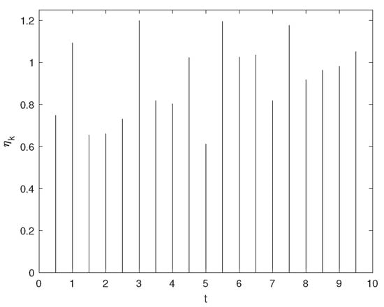
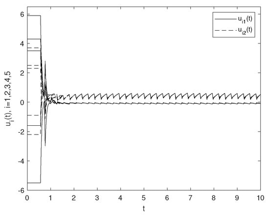
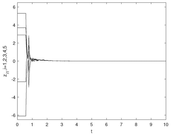
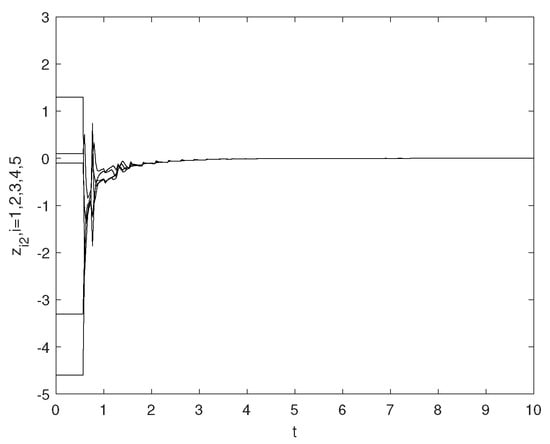
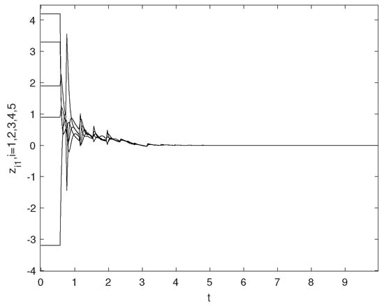
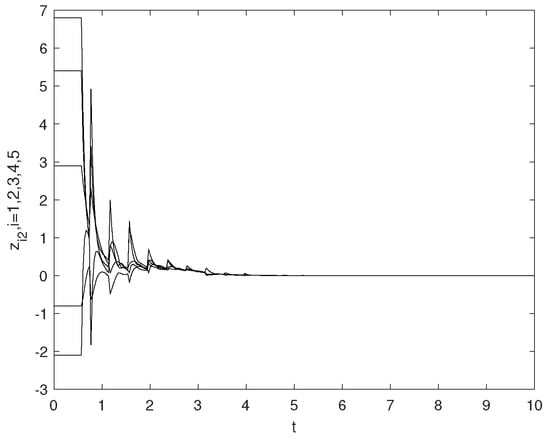
${\eta }_k$ is the stochastic impulsive intensity at $t_k$ satisfying the uniform distribution U(0.6, 1.2). Figure 1 shows the stochastic impulsive sequence ${\eta }_k$ with $T_a=0.5$ and $N_0=1$. Let $c=0.75$. The impulsive sequence is chosen as $t_k=0.5k,k\in N^{+}$. Apparently, $T_a=0.5,N_0=1$. By calculation, we can obtain that $Q=\mathrm{diag}\{0.8,0.8\}$, ${\displaystyle \overline{\alpha }}=0.9$, ${{\displaystyle \overline{\gamma }}}^2=0.03$, $\chi =0.8035$, $b=-\frac{{\lambda }_2({\displaystyle \overline{L}})}{{\lambda }_{\max }(W)}=3.6227$, $p=-{\lambda }_{\max }\left(D+D^T+A{A}^T+Q{Q}^T+B{B}^T+C{C}^T-\theta b\Gamma \right)=1.5836$, $q={\lambda }_{\max }(Q{Q}^T)=0.64$, $r={\sigma }_2{\lambda }_{\max }(Q{Q}^T)=0.32$, $M_1=\max \left\{c^{-\frac{{\sigma }_1}{T_a}-N_0},1\right\}=1.8831$, $M_2=\max \left\{c^{-\frac{{\sigma }_2}{T_a}-N_0},1\right\}=1.7778$, $\alpha ={\rho }_k({{\displaystyle \overline{\alpha }}}^2+{{\displaystyle \overline{\gamma }}}^2)=0.42$, and ${\gamma }^2={\rho }_k^2[\chi -{({{\displaystyle \overline{\alpha }}}^2+{{\displaystyle \overline{\gamma }}}^2)}^2]=0.0244$. Since $p>q{M}_1+r{M}_2{\sigma }_2=1.4896$, we can find that ${\displaystyle \overline{ϵ}}=0.052>0$ is the unique solution of equation $ϵ-p+q{M}_1{e}^{{\sigma }_1ϵ}+r{M}_2\frac{1}{ϵ}(e^{{\sigma }_2ϵ}-1)=0$. Furthermore, we can compute that $\lambda =\min \left\{\alpha {\rho }_k{e}^{{\displaystyle \overline{ϵ}}{\rho }_k}+\frac{c{\rho }_k^2{e}^{2{\displaystyle \overline{ϵ}}{\rho }_k}{\gamma }^2}{{(\alpha {\rho }_k{e}^{{\displaystyle \overline{ϵ}}{\rho }_k}-c)}^2},\alpha {\rho }_k{e}^{{\displaystyle \overline{ϵ}}{\rho }_k}+c\right\}=0.2324$. Noting that ${\displaystyle \overline{ϵ}}-\frac{\ln \lambda }{T_a}=1.3195$, all the conditions in Theorem 1 are satisfied, which signifies that system (75) can be exponentially synchronized in mean square. Figure 2 shows the state trajectories of all nodes, and the error trajectories $z_{i1},(i=1,2,3,4,5)$ and $z_{i2},(i=1,2,3,4,5)$ are shown in Figure 3 and Figure 4, respectively. It can be seen from Figure 2, Figure 3 and Figure 4 that the state trajectories of different nodes tend to be consistent.

Example 2.

Consider the coupled neural network system (75) with $u_i={(u_{i1},u_{i2})}^T,N=5,{\sigma }_1(t)=0.6\cos (t)\le {\sigma }_1=0.6,{\sigma }_2=0.5,\theta =1.8,J(t)={(1.2,3.6)}^T,0\le {\rho }_k=0.5=\rho ,g(u_i(t))=0.9(\tanh {(u_{i1}(t),\tanh (u_{i2}(t)))}^T,i=1,\dots ,N$. Meanwhile, the corresponding coefficient matrices and inner coupled matrix are selected below.

$$D=\left(\begin{array}{cc}-3& 0\\ 0& -3.6\end{array}\right),A=\left(\begin{array}{cc}1.9& 1.5\\ -1.6& 1.2\end{array}\right),B=\left(\begin{array}{cc}-1.9& 1.2\\ -1.6& 1.7\end{array}\right)$$

$$C=\left(\begin{array}{cc}0.3& -0.1\\ 0.4& 0.5\end{array}\right),\Gamma =\left(\begin{array}{cc}2.1& 0\\ 0& 1.5\end{array}\right),$$

and the outer coupling matrix is

$$L=\left(\begin{array}{ccccc}-3& 0& 1& 2& 0\\ 1& -2& 1& 0& 0\\ 0& 0& -4& 2& 2\\ 0& 1& 0& -3& 2\\ 1& 1& 0& 0& -2\end{array}\right).$$

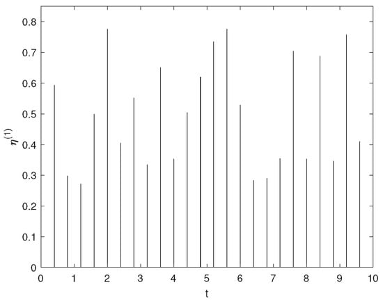
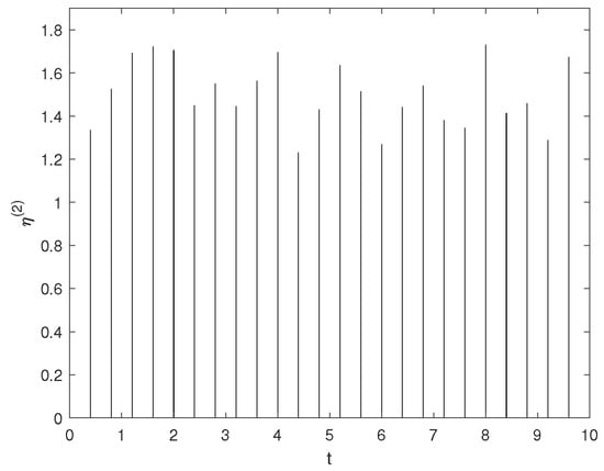
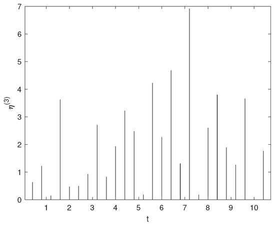
${\left\{{\eta }^{(i)}\right\}}_{i\in \Omega },\Omega \triangleq \{1,2,3\}$ denotes three kinds of different independent random variables and satisfy ${\eta }^{(1)}\sim U(0.2,0.8),{\eta }^{(2)}\sim U(1.2,1.8)$, and ${\eta }^{(3)}\sim E(1.6)$. Figure 5, Figure 6 and Figure 7 show the stochastic impulsive sequence ${\left\{{\eta }^{(i)}\right\}}_{i\in \Omega },\Omega \triangleq \{1,2,3\}$ with $T_a=0.5$ and $N_0=1$, respectively. A transition probability matrix is

$$P=\left(\begin{array}{ccc}0.2& 0.5& 0.3\\ 0.4& 0.3& 0.3\\ 0.3& 0.6& 0.1\end{array}\right),$$

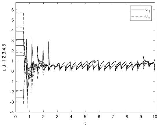
and ${\xi }_1=0.3125,{\xi }_2=0.4375,{\xi }_3=0.25$. Let $c=1$. The impulsive sequence is chosen as $t_k=0.4k,k\in N^{+}$. Apparently, $T_a=0.4,N_0=1$. By calculation, we can obtain that $Q=\mathrm{diag}\{0.9,0.9\}$, ${\mu }_1^{(i)}=0.5$, ${({\omega }_1^{(i)})}^2=0.03$, ${\chi }_1^{(i)}=0.1091$, ${\mu }_2^{(i)}=1.5$, ${({\omega }_2^{(i)})}^2=0.03$, ${\chi }_2^{(i)}=5.4691$, ${\mu }_3^{(i)}=0.625$, ${({\omega }_3^{(i)})}^2=0.3906$, ${\chi }_3^{(i)}=15$, $b=-\frac{{\lambda }_2({\displaystyle \overline{L}})}{{\lambda }_{\max }(W)}=3.8514$, $p=-{\lambda }_{\max }\left(D+D^T+A{A}^T+Q{Q}^T+B{B}^T+C{C}^T-\theta b\Gamma \right)=3.8202$, $q={\lambda }_{\max }(Q{Q}^T)=0.81$, $r={\sigma }_2{\lambda }_{\max }(Q{Q}^T)=0.4050$, $M_1=\max \left\{c^{-\frac{{\sigma }_1}{T_a}-N_0},1\right\}=1$, $M_2=\max \left\{c^{-\frac{{\sigma }_2}{T_a}-N_0},1\right\}=1$, ${\alpha }_1=\rho \left[{({\mu }_1^{(i)})}^2+{({\omega }_1^{(i)})}^2\right]=0.1400$, and ${\gamma }_1^2={\rho }^2\left[{\chi }_1^{(i)}-{({({\mu }_1^{(i)})}^2+{({\omega }_1^{(i)})}^2)}^2\right]=0.0077$, ${\alpha }_2=\rho \left[{({\mu }_2^{(i)})}^2+{({\omega }_2^{(i)})}^2\right]=1.1400$, and ${\gamma }_2^2={\rho }^2\left[{\chi }_2^{(i)}-{({({\mu }_2^{(i)})}^2+{({\omega }_2^{(i)})}^2)}^2\right]=0.0677$, ${\alpha }_3=\rho \left[{({\mu }_3^{(i)})}^2+{({\omega }_3^{(i)})}^2\right]=0.3906$, and ${\gamma }_3^2={\rho }^2\left[{\chi }_3^{(i)}-{({({\mu }_3^{(i)})}^2+{({\omega }_3^{(i)})}^2)}^2\right]=3.5974$. Since $p>q{M}_1+r{M}_2{\sigma }_2=1.0125$, we can find that ${\displaystyle \overline{ϵ}}=1.5115>0$ is the unique solution of equation $ϵ-p+q{M}_1{e}^{{\sigma }_1ϵ}+r{M}_2\frac{1}{ϵ}(e^{{\sigma }_2ϵ}-1)=0$. Furthermore, we can compute that ${\lambda }_1=\min \left\{{\alpha }_1\rho e^{{\displaystyle \overline{ϵ}}\rho }+\frac{c{\rho }^2{e}^{2{\displaystyle \overline{ϵ}}\rho }{\gamma }_1^2}{{({\alpha }_1\rho e^{{\displaystyle \overline{ϵ}}\rho }-c)}^2},{\alpha }_1\rho e^{{\displaystyle \overline{ϵ}}\rho }+c\right\}=0.1610$, ${\lambda }_2=\min \left\{{\alpha }_2\rho e^{{\displaystyle \overline{ϵ}}\rho }+\frac{c{\rho }^2{e}^{2{\displaystyle \overline{ϵ}}\rho }{\gamma }_2^2}{{({\alpha }_2\rho e^{{\displaystyle \overline{ϵ}}\rho }-c)}^2},{\alpha }_2\rho e^{{\displaystyle \overline{ϵ}}\rho }+c\right\}=2.2136$, ${\lambda }_3=\min \left\{{\alpha }_3\rho e^{{\displaystyle \overline{ϵ}}\rho }+\frac{c{\rho }^2{e}^{2{\displaystyle \overline{ϵ}}\rho }{\gamma }_3^2}{{({\alpha }_3\rho e^{{\displaystyle \overline{ϵ}}\rho }-c)}^2},{\alpha }_3\rho e^{{\displaystyle \overline{ϵ}}\rho }+c\right\}=1.4216$. $\zeta =1.3742$, ${ϵ}_0=0.1$. Noting that ${\displaystyle \overline{ϵ}}-\frac{\ln (\zeta +{ϵ}_0)}{T_a}=0.5412$, all the conditions in Theorem 1 are satisfied, which signifies that system (75) can be exponentially synchronized in mean square. Figure 8 shows the state trajectories of all nodes, and the error trajectories $z_{i1},(i=1,2,3,4,5)$ and $z_{i2},(i=1,2,3,4,5)$ are shown in Figure 9 and Figure 10, respectively. It can be seen from Figure 8, Figure 9 and Figure 10 that the state trajectories of different nodes tend to be consistent.

Remark 8.

In Examples 1 and 2, apart from stochastic distributed impulsive sequence, hybrid delays and coupled strengthen have been considered and discussed simultaneously. Particularly, when coupled strengthen θ become large, error trajectories will converge to zero vector more quickly. In references [34,35,36], although stochastic impulses have been considered, hybrid delays, coupled structure and stochastic distributed impulses have been ignored. Therefore, those theoretical results in [34,35,36] can not be directly to Examples 1 and 2, and by utilizing Theorems 1 and 2, we can verified that the exponential synchronization in mean square of CNNs is realized in Examples 1 and 2.

5. Conclusions

In this article, we have investigated the exponential synchronization of CNNs with hybrid delays and stochastic distributed delayed impulses. Some new criteria on the exponential synchronization in the mean square of CNNs are derived.

Firstly, two types of stochastic impulses, i.e., stochastic distributed delayed impulses with dependent property and Markov property have been taken into account, respectively. By utilizing the average impulsive interval method, total probability formula and ergodic theory, two novel Halanay differential inequalities with stochastic distributed delay impulses are established.

Secondly, based on the previous two novel impulsive Halanay differential inequalities, some sufficient conditions are acquired to guarantee the mean square exponential synchronization of CNNs.

Thirdly, the effectiveness of theoretical results is verified through two simulation examples, stochastic impulsive sequences, state trajectories of all the nodes and error trajectories have been shown through a series of figures.

However, semi-Markov jump CNNs or discrete CNNs with stochastic delayed impulses have not been investigated. Therefore, in the future, we can further explore the mean square exponential synchronization of semi-Markov jump CNNs or discrete CNNs with stochastic delayed impulses.

References

- Nishio, Y.; Ushida, A. Spatio-temporal chaos in simple coupled chaotic circuits. IEEE Trans. Circuits Syst. I Fundam. Theory Appl. 1995, 42, 678–686. [Google Scholar] [CrossRef][Green Version]
- Perez-Munuzuri, V.; Perez-Villar, V.; Chua, O.L. Autowaves for image processing on a two-dimensional CNN array of excitable nonlinear circuits:Flat and wrinkled labyrinths. IEEE Trans. Circuits Syst. I Fundam. Theory Appl. 1993, 40, 174–181. [Google Scholar] [CrossRef]
- Xiu, R.; Zhang, W.; Zhou, Z. Synchronization issue of coupled neural networks based on flexible impulse control. Neural Netw. 2022, 149, 57–65. [Google Scholar] [CrossRef] [PubMed]
- Mao, X.; Wang, Z. Stability switches and bifurcation in a system of four coupled neural networks with multiple time delays. Nonlinear Dyn. 2015, 82, 1551–1567. [Google Scholar] [CrossRef]
- Pecora, L.M.; Carroll, T.L. Synchronization in chaotic systems. Phys. Rev. Lett. 1990, 64, 821–824. [Google Scholar] [CrossRef] [PubMed]
- Liang, J.; Wang, Z.; Liu, Y.; Liu, X. Robust synchronization of an array of coupled stochastic discrete-time delayed neural networks. IEEE Trans. Neural Netw. 2008, 19, 1910–1921. [Google Scholar] [CrossRef] [PubMed]
- Wang, J.L.; Wu, H.N.; Huang, T. Pinning control strategies for synchronization of linearly coupled neural networks with reaction-diffusion terms. IEEE Trans. Neural Netw. Learn. Syst. 2016, 27, 749–761. [Google Scholar] [CrossRef] [PubMed]
- Chen, H.; Shi, P.; Lim, C.C. Exponential synchronization for Markovian stochastic coupled neural networks of neutral-type via adaptive feedback control. IEEE Trans. Neural Netw. Learn. Syst. 2017, 28, 1618–1632. [Google Scholar] [CrossRef]
- Wen, S.; Zeng, Z.; Chen, M.Z.Q.; Huang, T. Synchronization of switched neural networks with communication delays via the event-triggered control. IEEE Trans. Neural Netw. Learn. Syst. 2017, 28, 2334–2343. [Google Scholar] [CrossRef]
- Gao, C.; Wang, Z.; He, X.; Yue, D. Sampled-data-based fault-tolerant consensus control for multi-agent systems: A data privacy preserving scheme. Automatica 2021, 133, 109–847. [Google Scholar] [CrossRef]
- Zhang, L.; Liu, J. Exponential synchronization for delayed coupled systems on networks via graph-theoretic method and periodically intermittent control. Phys. A 2020, 545, 123–733. [Google Scholar] [CrossRef]
- Zhang, G.; Xia, Y.; Li, X.; He, S. Multievent-triggered sliding-Mode control for a class of complex dynamic network. IEEE Trans. Control Netw. Syst. 2022, 9, 835–844. [Google Scholar] [CrossRef]
- Fan, H.; Rao, Y.; Shi, K.; Wen, H. Global synchronization of fractional-order multi-delay coupled neural networks with multi-link complicated structures via hybrid impulsive control. Mathematics 2023, 11, 3051. [Google Scholar] [CrossRef]
- Rao, R.; Zhu, Q. Synchronization for reaction–diffusion switched delayed feedback epidemic systems via impulsive control. Mathematics 2024, 12, 447. [Google Scholar] [CrossRef]
- Xiao, Q.; Liu, H.; Wang, Y. An improved finite-time and fixed-time stable synchronization of coupled discontinuous neural networks. IEEE Trans. Neural Netw. Learn. Syst. 2021, 34, 3516–3526. [Google Scholar] [CrossRef]
- Li, P.; Cao, J.; Wang, Z. Robust impulsive synchronization of coupled delayed neural networks with uncertainties. Phys. A 2007, 373, 261–272. [Google Scholar] [CrossRef]
- Lu, J.; Ho, D.W.; Cao, J.; Kurths, J. Exponential synchronization of linearly coupled neural networks with impulsive disturbances. IEEE Trans. Neural Netw. 2011, 22, 329–335. [Google Scholar] [CrossRef] [PubMed]
- Yang, D.; Li, X.; Song, S. Finite-time synchronization for delayed complex dynamical networks with synchronizing or desynchronizing impulses. IEEE Trans. Neural Netw. Learn. Syst. 2022, 33, 736–746. [Google Scholar] [CrossRef]
- Wang, N.; Li, X.; Lu, J.; Alsaadi, F.E. Unified synchronization criteria in an array of coupled neural networks with hybrid impulses. Neural Netw. 2018, 101, 25–32. [Google Scholar] [CrossRef]
- Xu, H.; Zhu, Q.; Zheng, W.X. Exponential stability of stochastic nonlinear delay systems subject to multiple periodic impulses. IEEE Trans. Autom. Control 2023, 69, 2621–2628. [Google Scholar] [CrossRef]
- Hu, W.; Zhu, Q.; Karimi, H.R. Some improved Razumikhin stability criteria for impulsive stochastic delay differential systems. IEEE Trans. Autom. Control 2019, 64, 5207–5213. [Google Scholar] [CrossRef]
- Li, X.; Wu, J. Stability of nonlinear differential systems with state-dependent delayed impulses. Automatica 2016, 64, 63–69. [Google Scholar] [CrossRef]
- Liu, X.; Zhang, K. Synchronization of linear dynamical networks on time scales: Pinning control via delayed impulses. Automatica 2016, 72, 147–152. [Google Scholar] [CrossRef]
- Huang, Z.; Cao, J.; Li, J.; Bin, H. Quasi-synchronization of neural networks with parameter mismatches and delayed impulsive controller on time scales. Nonlinear Anal. Hybri. 2019, 33, 104–115. [Google Scholar] [CrossRef]
- Gao, K.; Lu, J.; Zheng, W.X.; Chen, X. Synchronization in coupled neural networks with hybrid delayed impulses: Average impulsive delay-gain method. IEEE Trans. Neural Netw. Learn. Syst. 2024; in press. [Google Scholar] [CrossRef]
- Liu, X.; Zhang, K. Stabilization of nonlinear time-delay systems: Distributed-delay dependent impulsive control. Syst. Control Lett. 2018, 120, 17–22. [Google Scholar] [CrossRef]
- Xu, Z.; Peng, D.; Li, X. Synchronization of chaotic neural networks with time delay via distributed delayed impulsive control. Neural Netw. 2019, 118, 332–337. [Google Scholar] [CrossRef]
- Zhang, X.; Li, C.; Li, H.; Cao, Z. Synchronization of uncertain coupled neural networks with time-varying delay of unknown bound via distributed delayed impulsive control. IEEE Trans. Neural Netw. Learn. Syst. 2021, 34, 3624–3635. [Google Scholar] [CrossRef] [PubMed]
- Fang, Q.; Wang, M.; Li, X. Event-triggered distributed delayed impulsive control for nonlinear systems with applications to complex networks. Chaos Soliton Fract. 2023, 175, 113–943. [Google Scholar] [CrossRef]
- Hu, W.; Zhu, Q. Stability criteria for impulsive stochastic functional differential systems with distributed-delay dependent impulsive effects. IEEE Trans. Syst. Man, Cybern. 2021, 51, 2027–2032. [Google Scholar] [CrossRef]
- Li, J.; Zhu, Q. Stability of neutral stochastic delayed systems with switching and distributed-delay dependent impulses. Nonlinear Anal. Hybri. 2023, 47, 101–279. [Google Scholar] [CrossRef]
- Tang, Y.; Wu, X.; Shi, P.; Qian, F. Input-to-state stability for nonlinear systems with stochastic impulses. Automatica 2020, 113, 108–766. [Google Scholar] [CrossRef]
- Liu, J.; Zhu, Q. Finite time stability of time-varying stochastic nonlinear systems with random impulses. Int. J. Control 2023. [Google Scholar] [CrossRef]
- Sun, Y.; Li, L.; Liu, X. Exponential synchronization of neural networks with time-varying delays and stochastic impulses. Neural Netw. 2020, 132, 342–352. [Google Scholar] [CrossRef]
- Cui, Q.; Li, L.; Cao, J. Stability of inertial delayed neural networks with stochastic delayed impulses via matrix measure method. Neurocomputing 2022, 471, 70–78. [Google Scholar] [CrossRef]
- Li, L.; Cui, Q.; Cao, J.; Qiu, J.; Sun, Y. Exponential synchronization of coupled inertial neural networks with hybrid delays and stochastic impulses. IEEE Trans. Neural Netw. Learn. Syst. 2023; in press. [Google Scholar] [CrossRef]
- Ling, G.; Liu, X.; Guan, Z.H.; Ge, M.F.; Tong, Y.H. Input-to-state stability for switched stochastic nonlinear systems with mode-dependent random impulses. Inf. Sci. 2022, 596, 588–607. [Google Scholar] [CrossRef]
- Zhang, N.; Huang, S.; Li, W. Stability of stochastic delayed semi-Markov jump systems with stochastic mixed impulses: A novel stochastic impulsive differential inequality. J. Franklin Inst. Eng. Appl. Math. 2022, 359, 10785–10812. [Google Scholar] [CrossRef]
- Ross, S.M. Stochastic Processes; John Wiley & Sons: New York, NY, USA, 1996. [Google Scholar]
- Lu, J.; Ho, D.W.C.; Cao, J. A unified synchronization criterion for impulsive dynamical networks. Automatica 2010, 46, 1215–1221. [Google Scholar] [CrossRef]
- Dong, S.; Shi, K.; Wen, S.; Shen, Y.; Zhong, S. Almost surely synchronization of directed coupled neural networks via stochastic distributed delayed impulsive control. Chaos Soliton Fract. 2023, 174, 113–742. [Google Scholar] [CrossRef]
Disclaimer/Publisher’s Note: The statements, opinions and data contained in all publications are solely those of the individual author(s) and contributor(s) and not of MDPI and/or the editor(s). MDPI and/or the editor(s) disclaim responsibility for any injury to people or property resulting from any ideas, methods, instructions or products referred to in the content. |
© 2024 by the authors. Licensee MDPI, Basel, Switzerland. This article is an open access article distributed under the terms and conditions of the Creative Commons Attribution (CC BY) license (https://creativecommons.org/licenses/by/4.0/).