Article

Reservoir Slope Stability Analysis under Dynamic Fluctuating Water Level Using Improved Radial Movement Optimisation (IRMO) Algorithm

School of Civil Engineering, Central South University, No. 68, Shaoshan South Rd., Changsha 410075, China
*
Author to whom correspondence should be addressed.
Mathematics 2024, 12(13), 2055; https://doi.org/10.3390/math12132055
Submission received: 6 May 2024 / Revised: 14 June 2024 / Accepted: 27 June 2024 / Published: 30 June 2024

Abstract

:
External water level fluctuation is the major trigger causing reservoir slope failure, and therefore it is of great significance for the safety assessment and corresponding safety management of reservoir slopes. In this work, the seepage effects stemming from fluctuating external water levels are given special analysis and then incorporated into the rigorous limit equilibrium method for assessing the stability of reservoir slope. An advanced metaheuristic intelligent algorithm, the improved radial movement optimisation (IRMO), is introduced to efficiently locate the critical failure surface and associated minimum factor of safety. Consequently, the effect of water level fluctuation directions, changing rates, and soil permeability coefficient on reservoir stability are investigated by the proposed method in three cases. It is found that the clay slope behaved more sensitively in stability fluctuation compared to the silty slope. With the dropping of external water, the higher dropping speed and lower soil permeability coefficient have worse impacts on the slope stability. The critical pool level during reservoir water dropping could be effectively obtained through the analysis. The results indicate that the IRMO-based method herein could effectively realise the stability analysis of the reservoir slope in a dynamic fluctuating reservoir water level, which could provide applicable technology for following preventions.

1. Introduction

The effects of groundwater seepage significantly influence the stability of most slopes, especially for those located in the reservoir area. In Japan [1], nearly 60 percent of the reservoir landslides occurred during the sudden drawdown of the reservoir water level, and the remaining 40 percent occurred during the rise period of the reservoir water level, including the initial reservoir impoundment. In China, the Three Gorges Conservancy project resulted in a large increase in the reservoir water level since 1994, and correspondingly, the number of landslide hazards increased in the first ten years, as shown in Figure 1. Accurately locating the potential reservoir slope failure and taking effective protective measures is always the main work to ensure the safety of reservoir area. The rainfall and fluctuating external water levels are usually seen as the main reasons for inside seepage changes and are therefore considered as main factors responsible for landslides and reservoir slope failure. For this issue, an effective method for analysing the influence of dynamic and fluctuating water levels on reservoir slope stability is presented in this work.
During the reservoir water level drawdown, in addition to the strength reduction in geomaterial, the higher water level within the reservoir slope results in the development of seepage force destabilising the slope. A variety of relative studies have investigated the effect of seepage induced by water level fluctuation or rainfall on the safety evaluation of slopes. There are four main methods used to carry out the safety evaluation of reservoir slopes: limit analysis method (LAM) [3,4,5]; limit equilibrium method (LEM) [6,7]; numerical analysis [8,9,10]; and probabilistic analysis [11,12]. Compared with FEM and probabilistic analysis method, which require complex pre-processing and high-quality computation power, the LEM is more easily applied in engineering practices to locate the critical failure surface for the stability evaluation.
To study the influence of varying reservoir water levels on the reservoir slope stability, it is necessary to obtain the relationship between the external water level and the seepage field inside of reservoir slopes, accounting for the seepage and seepage forces on slope stability. The determination of the phreatic surface is a crucial issue in the field of seepage, involving unconfined free surface seepage. Based on numerous slope examples from projects, scholars have made great progress in numerical analysis using the finite element method [13,14]. Using numerical analysis, Zhang et al. [15] studied the influence of the phreatic surface positions and matric suction on the seepage field. By coupling the seepage field and stress field, Zhang and Dai [16] found that the soil permeability and seepage boundary conditions would directly affect the slope stability. Mao et al. [17] investigated the change in seepage field and the distribution of unsaturated zones inside the reservoir slope, and then carried out the stability analysis considering saturated–unsaturated seepage based on the theory of unsaturated soil mechanics. Using the commercial software SEEP/W and SLOPE/W, Mandal, Li and Shrestha [14] used the Morgenstern–Price method to investigate the influence of the rising rate of the reservoir water level on the rock slope stability. Most numerical simulations are based on complex numerical models and simulation schemes. To be more applicable to a wide range of practical situations, some scholars simplified the calculation formula for the phreatic surface to yield a simplified seepage field which could be used to calculate the pore water pressure or conduct equivalent seepage analysis for stability analysis. Zheng et al. [18] obtained the simplified formula for calculating the phreatic surface under falling reservoir water levels based on the Boussinesq equations and further studied the difference between the analytical solutions and numerical solutions of the phreatic surface by finite element software PLAXIS [19]. Similarly, Sun et al. [20] used the polynomial expression to fit the phreatic surface equation to obtain a simpler method for practical applications, by which the influence of rainfall and reservoir water level fluctuation on reservoir slope stability is further investigated. Moreover, Deng et al. [21] simplified the actual flow direction in seepage into the horizontal direction and classified the slices of slope according to the phreatic surface position. The stability of the reservoir slope with different classifications is analysed using the simplified Janbu method. Lu and Chen [22] obtained the analytical solution of pore water pressure on the failure surface by assuming that the phreatic surfaces were parabolic; by using the simplified Bishop method, the circular critical failure surface (CFS) and the corresponding factor of safety (FS) were determined for the slopes under two-dimensional steady seepage.
The search and determination of the CFS are essential parts of the slope stability analysis, which is usually presented as an unconstrained and complex nonlinear global optimisation problem. With the consideration of seepage effects, the problem will become more complicated, and higher requirements are put forward for the computation and optimisation performance. Compared with several traditional methods, such as the calculus of variation method, grid search method, golden section method, and random search method [23], the global optimisation algorithm showed great advantages in solving multi-dimensional objective functions with high efficiency and great accuracy, which could be effectively applied to search the CFS with minimum FS. In reviewing the existing literature, a variety of optimisation techniques have been integrated with various seepage analysis approaches to enhance the analysis of slope stability by accounting for seepage effects, as concluded in Table 1. Despite the efforts to successfully apply these methods, there remain some limitations associated with existing seepage analysis methods as well as each optimisation algorithm. As shown in Table 1, the pore–water pressure was commonly used in the calculation to approach the equivalent consideration, which made it hard to realise the actual interaction between water and earth in the slope. Additionally, difficulties remain in the selection of parameters in the Genetic Algorithm (GA) [24,25,26], the low searching efficiency in the Ant Colony Optimisation (ACO) algorithm [27,28], and the poor convergence and instability in the Particle Swarm Optimisation algorithm (PSO) [29,30,31] and Simulating Annealing algorithm (SA) [32]. These challenges make it difficult to achieve ideal global optimisation (easily falling into local optimal solutions), as each algorithm has its limitations [33]. Therefore, many scholars have endeavoured to enhance these existing algorithms to explore more efficient and precise ways that are better suited for more complex slope stability analysis in conditions of seepage effect [34].
The Radial Movement algorithm (RMO) [37] is a novel metaheuristic algorithm with the advantages of simple progress, taking up little storage and convergence quickly for application. But when it comes to the slope stability with LEMs, it was difficult for the RMO algorithm to obtain stable results for searching CFS with a minimum FS. It was found that it easily ignores the self-feedback of the particles and loses the particle information which contributes to poor performance in search precision and stability. To overcome these limitations, Jin et al. (2016) [38] improved its data structures and proposed a new method, namely the Improved Radial Movement Optimisation (IRMO), which has shown great stability and accuracy in slope stability analysis combined with the imbalance trust method [38], the Morgenstern–Price method [39], and the Spencer method [40]. Moreover, the IRMO algorithm has been found to be suitable for employing the slope stability analysis with seepage flows, as per previous studies [36]. Summarised findings from the comparison with alternative competitive optimisation methods are outlined in Table 2 and Table 3. And the results related to the IRMO are highlighted in bold. As shown in Table 2, the IRMO algorithm can achieve a significantly lower minimum FS compared to most existing optimisation techniques, which indicates its substantial advantages in solving this kind of complex nonlinear analytical problem. The IRMO algorithm can also yield more stable computation results over 20 trials (Table 3). It suggests that the IRMO algorithm exhibits great efficiency, superior stability, and accuracy in searching CFS for such reservoir slopes affected by seepage. With the support of the above research results, the reservoir slope stability analysis under fluctuating external water levels is further investigated based on the IRMO algorithm in this paper.
In the present study, the hysteresis effect of the seepage field within a slope related to the reservoir water level fluctuation is being considered. The phreatic surface expressions during the decline of the reservoir water levels are derived according to Boussinesq Equation and subsequently fitted with a parabola for engineering applications. The mechanical expression of the seepage force is accordingly derived based on static equilibrium analysis. Comprehensively, by utilising the phreatic surface of the slope under fluctuating reservoir water levels, the seepage force equation, and the limit equilibrium method (rigorous Janbu method), an integrated approach for analysing reservoir slope stability under seepage force is proposed and implemented by programming based on the advanced IRMO algorithm. The IRMO algorithm has been proven to be highly efficient and robust, making it suitable for solving complex problems related to reservoir slopes. Finally, by applying these methods to several typical reservoir slope cases, the assessment of reservoir slope stability is further investigated in terms of different reservoir water fluctuation directions (i.e., rising or dropping), changing the rates of the reservoir water level and soil permeability coefficients.

2. Rigorous Limit Equilibrium Analysis Considering Seepage Force

The change of seepage field induced by external water level fluctuation is the main reason that causes the changes in reservoir slope stability. However, it is always challenging to depict the actual seepage field and obtain a precise seepage analysis. In previous studies, the pore water pressure is generally used to equivalent the effects of groundwater seepage. It can be confusing at times whether to take into account a void ratio when calculating the seepage force. To accurately calculate the seepage force, which is the drag force created by the water on the soil particles under the action of seepage, this paper started the seepage force analysis according to the water pressure acting on each slope slice boundary. The limit equilibrium method (rigorous Janbu method) was further expanded with the seepage analysis under the fluctuating external water levels, and then carried out the reservoir slope stability analysis results.

2.1. Seepage Analysis

2.1.1. Relationship of Phreatic Surface and Fluctuating External Water Level

In practice, most seepage analysis regarding reservoir slopes (as well as foundation pits and dams) are usually assumed as the two-dimensional seepage problem occurring in the plane parallel to the seepage direction. Following the fundamental assumptions outlined below, the phreatic surfaces within the reservoir slope induced by external water level fluctuations were determined and then employed to calculate the seepage force within slope slices.
Basic assumptions for the determination of phreatic surface:
  • The reservoir slope is considered a vertical slope. The reservoir slope within the declining amplitude is much smaller than the ground, so it is considered a vertical slope for simplification.
  • The change in phreatic flow parallel to the slope surface is caused by the reservoir water-level fluctuation. (The change in phreatic flow perpendicular to the slope surface caused by the rainfall infiltration is not considered herein.)
  • The external reservoir water level is decreasing or increasing at a constant speed of V0.
  • The aquifer within the slope is homogeneous and isotropic with an infinite lateral extension.
Based on the above assumptions, the phreatic surface can be obtained by the Boussinesq Equation, which can be written as:
u t = k h m μ 2 u x 2 x > 0 , u > 0 ,
where x is the coordinate axis; μ is the specific yield; hm is the average value of the aquifer thickness; u is the water head at time t; t is time; k is the soil permeability coefficient.
By applying the Laplace transformation and its inverse transformation, the solution of Equation (1) could be expressed as:
u ( x , t ) = V 0 t 1 + 2 λ 2 E r f c λ 2 π λ e λ 2 ,
where λ = x / 2 μ / k h m t , E r f c λ is the residual error function, E r f c λ = 2 / π λ e λ 2 d x .
Thus, the phreatic surface in the reservoir slope when the external water level drops at the same speed V0 can be further derived as [20]:
h x , t = h 0 , 0 u ( x , t ) ,
where hx,t is the expression of the phreatic surface line at time t and h0,0 is the phreatic surface level before the reservoir water drawdown.
However, the u(x, t) is so complex to calculate directly without using integral in the practices. To facilitate the engineering practices, a polynomial was used to fit the phreatic surface in the calculation. The simplified calculation formula of the phreatic surface was consistent with the results of finite element calculation under the same condition, therefore verifying its correctness [18]. Accordingly, the parabola is used in this work to simplify the calculation of fluctuating phreatic surfaces for seepage analysis.

2.1.2. Simplification of Seepage Field

In the seepage analysis, the flow function and potential function of the seepage field can be obtained as the phreatic surface has been determined, and therefore analyse the seepage force of divided slices. Due to simplifying the phreatic surface as a parabolic expression in this study, the potential function perpendicular to it becomes a complex curve, which brings some difficulties to determining the seepage force of each slope slice. To facilitate the programming calculation, the parabola phreatic surface is fitted by multiple micro-segments to determine the paralleled flow function and perpendicular potential function, the simplified seepage field as shown in Figure 2. According to the simplified seepage field, the seepage force of each slope slice could be determined by the static equilibrium analysis. The micro-segments of the parabolic phreatic surface are consistent with the divided slices of the slide body, which ensures the accuracy of seepage analysis in the slope under a specific seepage field. For sufficiently small widths of each slice and the phreatic surface segment, the reliability of the seepage analysis and slope stability analysis could be achieved simultaneously.

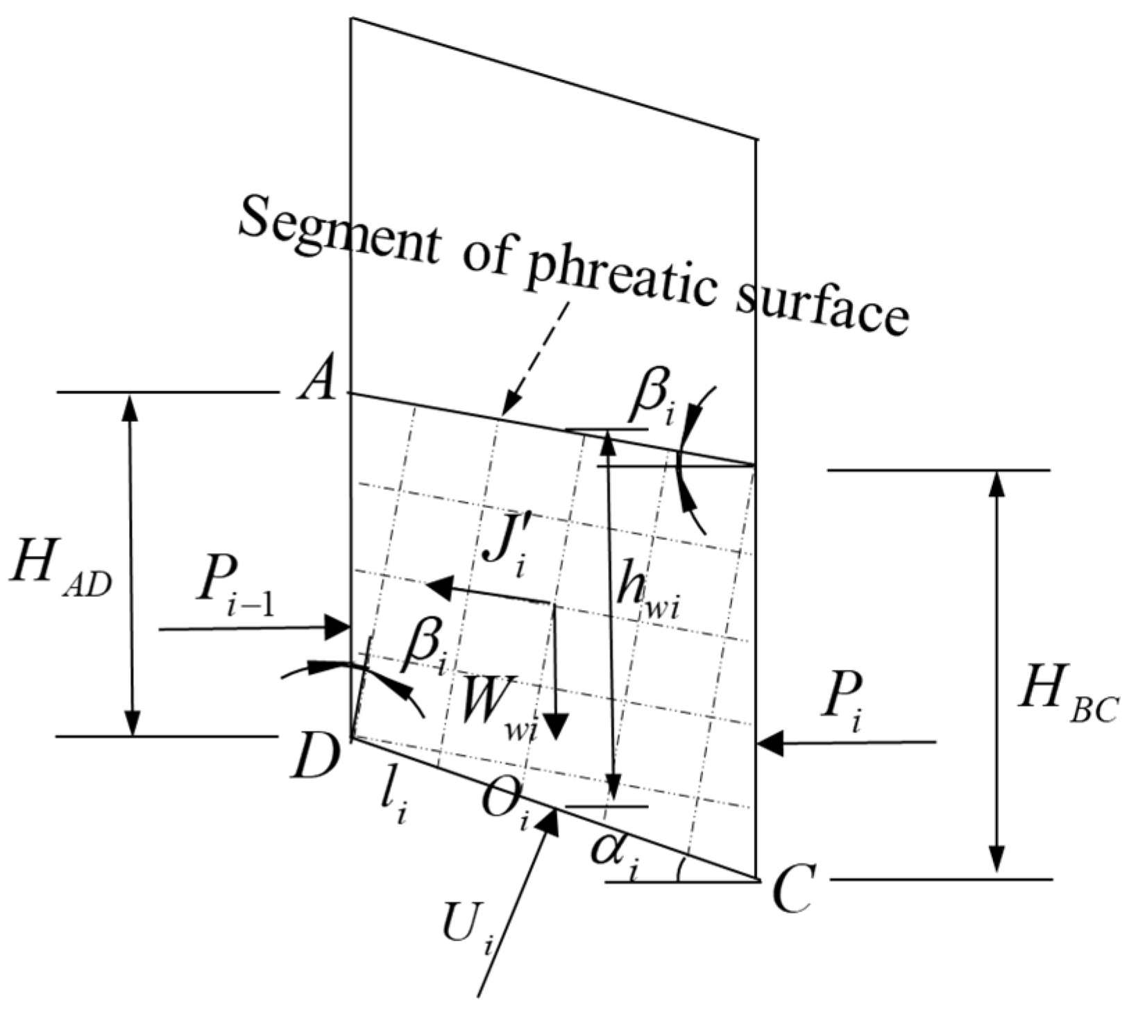
2.1.3. Seepage Force Analysis

On the basis of the simplified seepage field, the seepage force of each slope slice could be carried out as follows. As shown in Figure 3, the effective interaction force between soil and water is considered as the seepage force by analysing the soil skeleton and water body of each slice separately. Based on the static equilibrium conditions of the water body below the phreatic surface, the seepage force in the horizontal and vertical directions could be determined.
In Figure 3, Pi is the pore water pressure; HAD and HBC are the heights of the phreatic surface at sides; Ui is the pore water pressure at the slice base; hwi is the phreatic surface average height; βi is the phreatic surface inclination angle; αi is the base inclination angle; J’i is the reacting force of seepage force; Wwi is the unit weight of groundwater; and l i is the slice base length.
For the i-th slice, the force static equilibrium along the x direction is
U i sin α i J i x + P i 1 P i = 0 ,
the force static equilibrium along the y direction is:
W w i U i cos α i J i y = 0 ,
where
U i = γ w l i h w i cos 2 β i P i = 1 2 γ w H B C 2 cos 2 β i P i 1 = 1 2 γ w H A D 2 cos 2 β i ,
By incorporating the Ui, Pi, and Pi−1 with respect to other parameters into Equations (4) and (5), the component of seepage force Ji in horizontal and vertical directions could be expressed as:
J i x = γ w h w i cos 2 β i H A D H B C + l i sin α i J i y = J i y = γ w h w i sin 2 β i l i cos α i ,
According to the geometric condition,
H A D + l i sin α i H B C l i cos α i = tan β i ,
The seepage force Ji could be expressed as Equation (9):
J i = J i = J i y sin β i = γ w h w i l i sin β i cos α i ,
When it comes to the slice method, it is necessary to divide the sliding body into as many slices as possible to ensure the accuracy of the calculation. Therefore, once the slice width is small enough, the vertical forces, pore water pressure Ui, and contact pressure Ni in the slice can be considered to all pass through the slice base centre Oi. The moment equilibrium around Oi could be simplified as
P i 1 1 3 H i 1 + 1 2 l i sin α i P i 1 3 H i 1 2 l i sin α i J i cos β i L y = 0 ,
where the action location of the seepage force Ly could be expressed as
L y = P i 1 1 3 H i 1 + 1 2 l i sin α i P i 1 3 H i 1 2 l i sin α i J i cos β i ,
As the width of the slice is small enough, it could be assumed that Hi = Hi−1 = hwi, and therefore the action location of seepage force Ly could be deprived as:
L y = 1 2 h w i ,

2.2. Rigorous Janbu Method Combined with Seepage Force

The commonly used limit equilibrium strip method includes the Bishop method, Spencer method, Morgenstern–Price method, Janbu method, etc. Different methods have different assumptions and applicable conditions. Compared to the conventional Janbu method, the Rigorous Janbu method strictly considers both static equilibrium and moment equilibrium conditions to improve the accuracy of calculation, which is suitable for locating both the non-circular failure surface and circular failure surface. On the basis of the rigorous Janbu method, the seepage force obtained above is further added to the force analysis of slope slices for calculating the FS.
As shown in Figure 4, Ei is the normal forces; Ti is the shear forces; hi is the heights of action position of normal forces Ei; Wi1 is the unit weight of the slice part over the phreatic surface; W i 2 is the submerged unit weight of the slice part below the phreatic surface; Ni is the normal force acting at the base of the slice; Si is the shear force acting at the base of the slice; Ji is the seepage force; αi is the base inclination angle; and βi is the phreatic surface inclination angle.
For the i-th slice, the moment equilibrium equation around the base centre Oi could be written as:
T i + T i 1 l i cos α i 2 + E i h i 1 2 l i cos α i tan α i E i 1 h i 1 + 1 2 l i cos α i tan α i J i h w i cos β i 2 = 0
Substitute ΔEi = EiEi−1 and ΔTi = TiTi−1 into Equation (13), and ignoring the high-order of minuteness related to shear force increment ΔTi, the shear force Ti can be obtained as follows:
T i = J i h w i cos β i 2 l i cos α i E i h i h i 1 l i sin α i + Δ E i h i 1 + 1 2 l i cos α i tan α i l i cos α i ,
For the i-th slice, the static equilibrium equation along the horizontal direction and vertical direction could be written as
N i sin α i S i cos α i + J i cos β i + E i 1 E i = 0 W i 1 + W i 2 N i cos α i S i sin α i + J i sin β i + T i 1 T i = 0 ,
According to the Mohr–Coulomb criterion, the relationship between shear force and normal force is
S i = N i tan φ i F S + c i l i F S ,
In the condition of static equilibrium from Equation (15), the relationship of normal force increment ΔEi and factor of safety FS considering the seepage force can be concluded as the following implicit expression:
Δ E i = ( W i 1 + W i 2 Δ T i ) tan α i + J i sin β i tan α i + J i cos β i sec 2 α i F S + tan φ i tan α i ( W i 1 + W i 2 Δ T i ) tan φ i + J i sin β i tan φ i + c i l i cos α i ,
where φi is the internal friction angle and ci is the cohesive strength.
Without any external force acting on the assumed slide body, all of the normal force increments could be offset to zero, ΣΔEi = 0, as shown in Equation (16), which only contains two unknown parameters, F S and ΔTi. With an assumed initial value ΔTi = 0, the FS can be iteratively corrected to the minimum value by the Newton iteration method. The iteration calculation process is presented as follows:
Δ E i = ( W i 1 + W i 2 Δ T i ) tan α i + J i sin β i tan α i + J i cos β i sec 2 α i c i l i cos α i + ( W i 1 + W i 2 Δ T i ) tan φ i + J i tan φ i sin β i F S + tan φ i tan α i = 0 ,
Iterative computation process:
  • Assuming ΔTi = 0 at the beginning, there is only FS unknown in Equation (18).
  • Using the Newton iteration method, the initial FS1 can be obtained by Equation (18).
  • Substitute the initial FS1 and assumed ΔTi into Equation (17) to obtain the value of ΔEi and Ei.
  • According to Equation (14), the ΔTi and Ti can be updated iteratively with known ΔEi and Ei.
  • Repeat steps (1)–(2) above, the FSk can also be updated with the Newton iteration method.
  • If FSkFSk−1 < δ, δ is the requirement of calculation accuracy set in advance, the FSk will be output as the final result. Otherwise, repeat steps (3)–(5) above until the calculation accuracy is satisfied.

2.3. Non-Circular Critical Failure Surface Model

Regarding the slope stability analysis above, the IRMO algorithm is applied to search the CFS according to the non-circular model [25]. As shown in Figure 5, any non-circular failure surfaces can be determined by the initial horizontal distance d, the initial vertical deflection angle α1, and inclination increments Δαi. Thus, any non-circular failure surface can be represented by an N-dimensional vector for iterative computation, as shown in Equation (19).
x i = d     α 1     Δ α 2     Δ α 3         Δ α n s . t   :     d min < d < d max   10 ° < α 1 < 70 °     0 ° < Δ α i < 30 ° ,
For each assumed non-circular failure surface modelled as Figure 5 and Equation (19), the corresponding FS will be calculated by the Rigorous Janbu method following the iteration process above. By setting Equation (20) as the objective function, the FS of the M potential non-circular failure surfaces will be automatically calculated, compared, and updated in the IRMO algorithm. As the iteration ends with the terminate conditions, the optimal solution (the non-circular failure surface with minimum FS solution) will be output as the final CFS of the slope.
Objective   function : min : f ( X ) = f ( X M , N ) = f ( F S ) = Δ E i ,
where the variable matrix X M , N = x 1 x i x M T , M is the number of potential non-circular failure surfaces for each iteration, N is the number of all variables for each potential non-circular failure surface, N = n + 1.

3. Improved Radial Movement Optimisation (IRMO) Algorithm

3.1. Introduction of IRMO Algorithm

IRMO is a newly proposed global optimisation algorithm developed from the Radial Movement Optimisation (RMO) [37], which is designed to quickly find the optimum solution for nonlinear optimisation problems, such as locating the critical failure surface and determining the ultimate bearing capacity of the foundation [36,38,39,40]. After the objective function and variables’ matrix are determined, IRMO will randomly generate multiple particles (potential critical failure surfaces herein) and obtain the corresponding function values (value of FS herein). By comparing the function values, the optimum solution will be selected to be the central particle Center to guide the evolution of the particles, which could be called the radial movement. But, in IRMO, the particles are not completely governed by the Center when new particles are generated, whereas RMO is. To enhance the self-feedback iteration for generating high-quality new particles, some particles in IRMO holding excellent position information (variables’ value) could directly be inherited by the next generation. The stability of the algorithm can be greatly improved while the precision of the solution can be ensured.
According to previous studies, the IRMO algorithm has been proven to have great stability and accuracy in locating the CFS with a minimum FS for some classical slope problems. In this work, with the help of the IRMO, the CFS and corresponding minimum FS of the reservoir slope will be efficiently located to explore the effect of a dynamic fluctuating water level on the reservoir slope stability. The framework of the IRMO algorithm is detailed in Table 4.

3.2. Computation Process of the IRMO Algorithm

The process details of the IRMO algorithm follow the steps below:

3.2.1. Initialisation

x i = x i , 1 x i , j x i , N ,
x i , j = min x j + rand ( 0 , 1 ) × ( max x j min x j ) ,
In IRMO, every particle can be mathematically represented by an N-dimensional vector x i , as shown in Equation (21), which contains all the variables for getting a potential solution by the fitness function. At the beginning of the iterative computation, the value of each variable in x i is randomly generated within their constraint ranges as Equation (22), where the constraint ranges minxj and maxxj (1 ≤ jN) have been set in advance. The population size will be controlled within M particles aiming to find the optimal solution from the M constantly updated potential solutions. The corresponding variables matrix can be written as [XM, N], as shown in Equation (23).
X M , N = x 1 , 1 x 1 , 2 x 1 , N 1 x 1 , N x 2 , 1 x 2 , 2 x 2 , N 1 x 2 , N x M , 1 x M , 2 x M , N 1 x M , N ,
By Equation (20), calculating and comparing the fitness values f([XM,N])1 of the initial particles, the particle with the optimal fitness value (minimum FS) is set as the initial central particle Center1 and global optimal solution Gbest for the evolution.

3.2.2. Evolution: New Particles Updated

To enhance the self-feedback of particles (preservation of excellent particles), there are two different ways for particle evolution provided in the IRMO algorithm, updated by the central position or directly inheriting the information of old particles. Two random parameters, r1 and r2 = rand (0, 1), will be used to decide the updating way here. If r1 < R or r2 < P, new positions are produced around the Center by Equation (24), R is the probability of mutation set in advance, and P is the ratio of the N with the number of effective variables of the old particle. Otherwise, by Equation (25), calculate the fitness values f(Xik) of new particles in [XM,N]k and the contemporary optimal fitness value of the new group will be selected as Rbestk first. If the Rbestk is better than the existing Gbest, then update the information of the global optimal solution Gbest.
x i , j k = w k × rand ( 0.5 , 0.5 ) × ( max x j min x j ) + C e n t e r j k 1 ,
x i , j k = x i , j k 1 ,
where wk is the dynamically changing weight decreasing with the generation k increasing, as shown in Equation (26). The G is the value of the generation which is set in advance.
w k + 1 = w max ( w max w min ) 2 k G k G 2 , f G b e s t f R b e s t k W w k + 1 = w max ( w max w min ) k G 2 , f G b e s t f R b e s t k < W ,
By using this weight decreasing model, the IRMO algorithm can adjust the optimisation strategy during evolution according to the population quality. This allows it to adapt to the complex nonlinear variations when solving objective functions.

3.2.3. Evolution: Radial Movement of the Central Particle

To ensure the central particle’s prominent position in the global search direction and reduce the likelihood of getting stuck in a local optimum, the C e n t r e k is defined to be updated by contemporary optimal solution Rbestk−1 and global optimal solution Gbest, as shown in Equation (27),
C e n t e r k = C e n t e r k 1 + C 1 × ( G b e s t C e n t e r k 1 ) + C 2 × ( R b e s t k 1 C e n t e r k 1 )
where C1 and C2 are the coefficients affecting the convergence speed and accuracy of the algorithm. For the RMO algorithm, The values of C1 and C2 are generally chosen in the range of 0.4–0.9 for different objective functions [37]. In this study, C1 and C2 are set as 0.4 and 0.5 to balance the exploration and exploitation performance of IRMO according to previous studies [36,38,39,40].

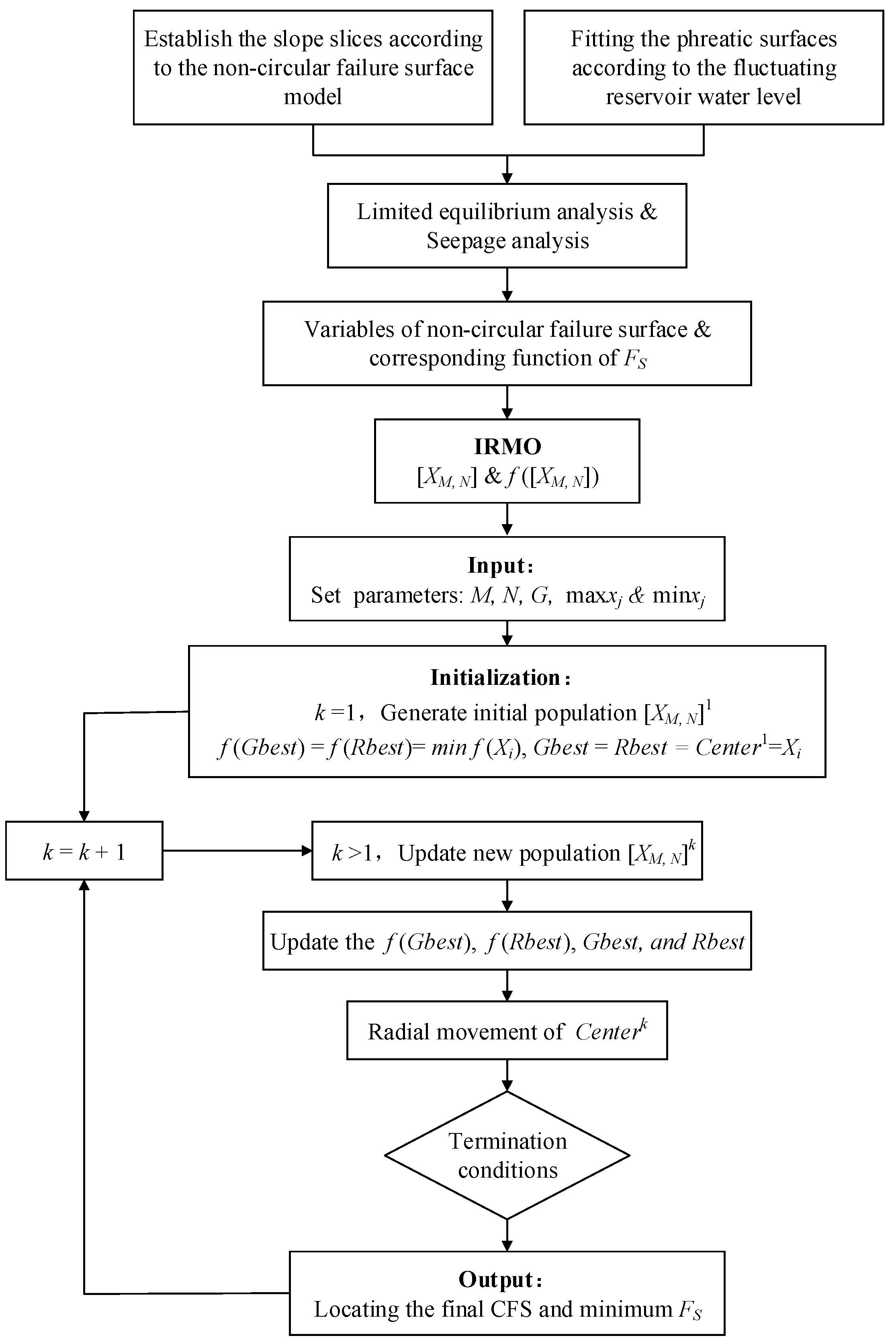
3.3. Implementation of IRMO Algorithm for Reservoir Slope Stability Analysis

Based on the slope modelled in Equation (19) and the implicit function of FS expressed in Equation (18), the reservoir slope stability could be efficiently analysed with the implementation of the IRMO algorithm. Following the evolution steps outlined above, the CFS and minimum FS of each reservoir slope with fluctuating external water levels could be determined. The algorithm parameters M (population size), N (the number of variables), and G (the maximum number of generations) have been tuned in advance to release the algorithm’s performance, where the details of parameters tuning could be referred to reference [36], as presented in Table 5. The implementation flowchart of the IRMO-based reservoir slope stability analysis in the condition of fluctuating external water level is shown in Figure 6.

4. Case Studies

To demonstrate the impact of seepage force on the slope stability, a standard slope model with phreatic surfaces is first analysed with and without considering the seepage force, respectively. The results are then compared with existing methods in the literature. Furthermore, based on the IRMO algorithm and the rigorous Janbu method considering seepage effects, this section analysed the stability of various reservoir slope conditions under reservoir water level fluctuations. The influences of the reservoir water level fluctuation direction, fluctuation rate, and soil permeability coefficient on the reservoir slope stability are investigated for both silt slopes and clay slopes.

4.1. Comparative Analysis of the Impact of Seepage Force

This case involves a homogeneous slope model with a gradually decreasing water table. The groundwater flows out from the foot of the slope and remains at the same elevation as the ground surface. The soil properties are as follows: γ = 18 kN/m3, c = 20 kPa, φ = 10°. The geometrical configuration of the slope model is depicted in Figure 7 below.
In previous studies, Pham and Fredlund [41] compared their DYNPROG program with other LEMs and commercial software for this slope case, while only considering the distribution of pore–water pressures during the slope stability analysis. Qin [42] conducted a mechanical analysis of seepage within this slope for stability analysis as well. However, the analysis only located the circular CFSs without any assistance from optimisation technology. Moreover, to illustrate the impact of seepage force on slope stability, this slope case was analysed with and without considering the seepage force using the IRMO algorithm, respectively. The locations of CFSs obtained by different methods are presented in Figure 7 as well.
It is observed that the location of the non-circular CFS obtained by IRMO which considers the seepage force, is highly similar to most previous research, regardless of whether those methods considered the seepage force or only considered the pore–water pressures. However, the non-circular CFS without considering seepage force is located in a shallower position with a smaller potential sliding volume. The detailed comparison and corresponding minimum FS values for each method are summarised in Table 6. The results obtained by the IRMO are highlighted in bold.
As shown in Table 3, without considering seepage force, the minimum FS obtained by the IRMO algorithm is 1.181, which is slightly higher than the results for other methods (on average by +3.4%). While considering the seepage force, the minimum FS calculated by IRMO is 1.007, which is significantly lower (on average by −20.6%) than the results obtained by the other methods, regardless of whether those methods considered the seepage force or considered the pore–water pressures only. Although Qin [42] also adopted the rigorous Janbu method while considering seepage force and obtained a result (FS = 1.178) close to the result of this study, which did not consider seepage force (FS = 1.181), they only analysed a fixed circular CFS instead of conducting a global search through an optimisation algorithm, as in this paper. It could be concluded that the IRMO demonstrates excellent performance in locating an effective hazardous CFS with a lower minimum FS due to its superior global search capability.

4.2. Effect of Varying Fluctuation Direction and Rate

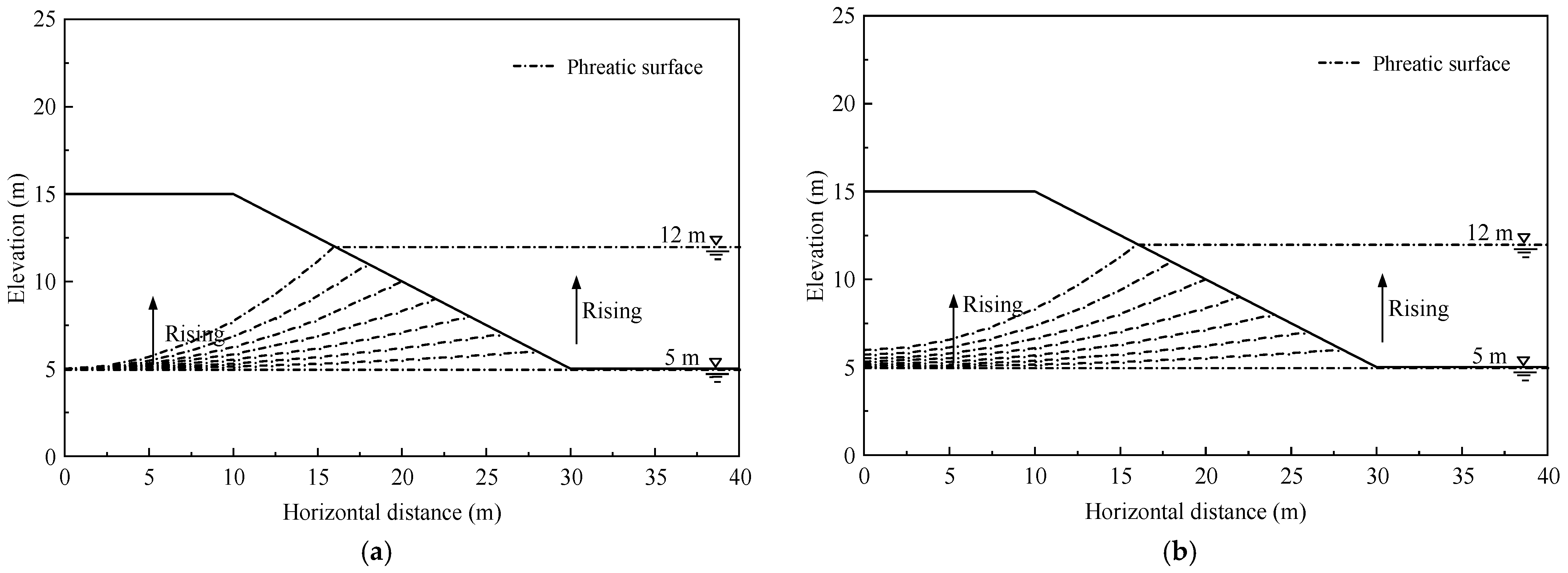
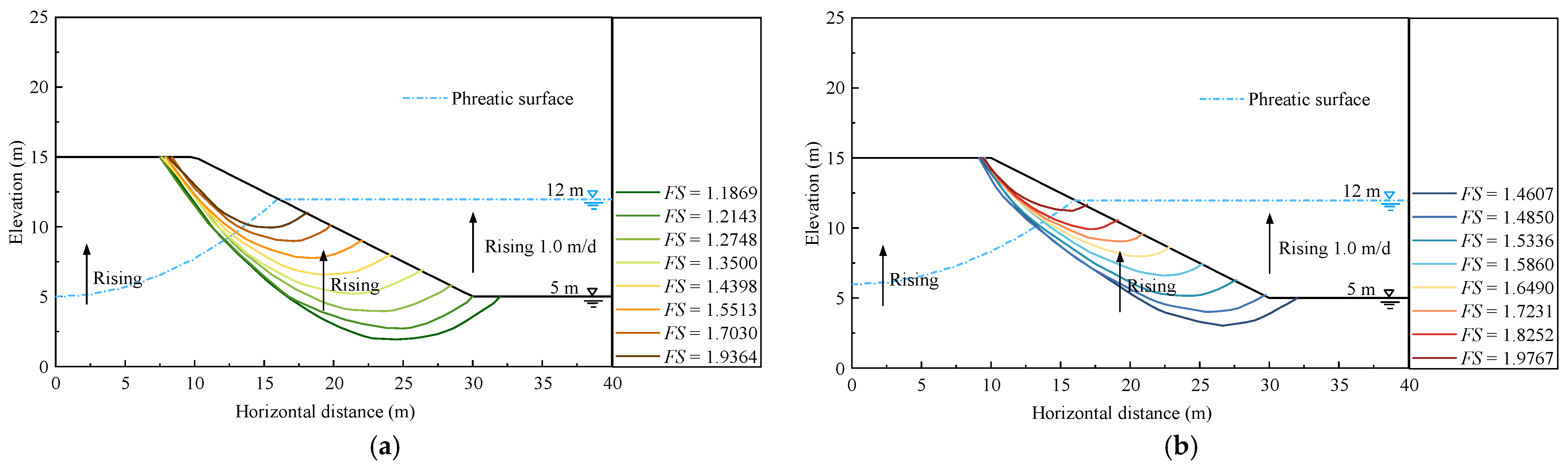
4.2.1. Effect of Reservoir Water Level Rising with Different Rates

This case is the silt slope and clay slope from Jiang [46]. Table 7 shows the related soil properties of the slopes.
Under the same water level fluctuation, the phreatic surface inside the slope exhibits significant positional differences, as shown in Figure 8 and Figure 9. In general, the water level inside the slope lags behind the water level outside during the process of the external water level rising, which is known as the hysteresis of the phreatic surfaces [18]. In the same slope with the same permeability coefficient k, the hysteresis will be more pronounced with the higher water level rising rate (such as Figure 8a and Figure 9a). However, with the same water level rising rate, the hysteresis of the phreatic surfaces in clay slope is more pronounced due to a lower permeability coefficient (as illustrated in Table 2, Figure 8 and Figure 9).
Using the IRMO algorithm to search the non-circular critical failure surfaces of the slope models in the condition of each position of the phreatic surface and calculate the corresponding minimum FS, the results are shown in Figure 10 and Figure 11.
It could be found that both the clay slope and silt slope exhibited the retrogressive failure mode. With the rising reservoir water level, the endpoint of the non-circular failure surface rises while the upper-end point moves slightly towards the slope edge, and the slide body becomes smaller. Figure 12 shows the change in minimum FS in such processes.
As shown in Figure 13, the minimum FS increases with the rising reservoir water level, and the increasing rate increases with a higher rising rate as well. For different soil slopes, the influence of the rising rate on the silt slope is greater than that of the clay slope. Comparing the calculated results with the previous study by Jiang [46], as shown in Figure 13, it could be found that the calculated FS values of this study are smaller than Jiang [46]. This is because the matric suction effect was not considered in this study. But it also proves that the matric suction is beneficial for slope stability during the rising of reservoir water level, especially in low water levels [46].

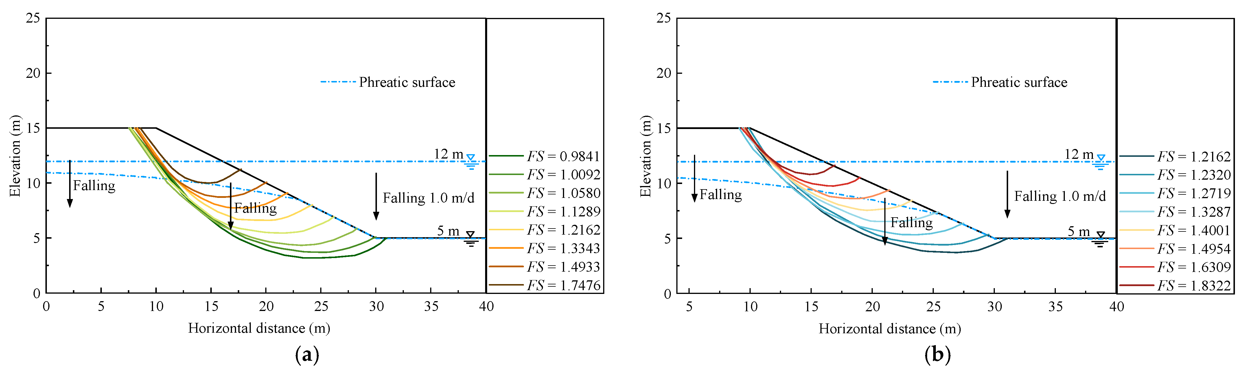
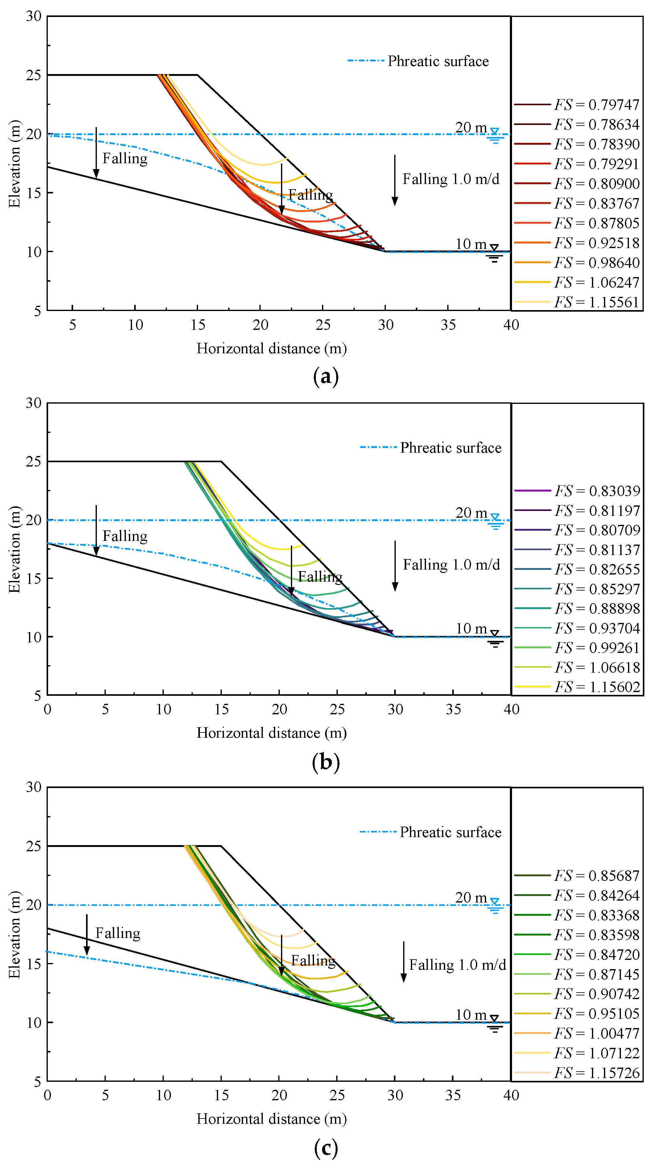
4.2.2. Effect of Reservoir Water Level Dropping

When the reservoir water level drops, the positions of the corresponding phreatic surface are shown in Figure 14 and Figure 15.
Similarly to the cases of rising reservoir water levels, the phreatic surfaces exhibited a pronounced hysteresis phenomenon to varying degrees as well, which are especially significant in the case of clay slope at a drop rate of 1.0 m/d, as shown in Figure 15a. By IRMO-based programming analysis, the non-circular CFSs of the slope models in the condition of each position of the phreatic surface are shown in Figure 16 and Figure 17.
Similarly to the cases of rising reservoir water level, with the dropping of the reservoir water level, the end point of the non-circular failure surface drops while the upper end point slightly moves away from the slope edge, and the slide body becomes larger. Figure 18 shows the change in minimum FS in such processes.
As shown in Figure 18, the minimum FS of silt slope decreases by 23.53% and 33.62% when the water level drops at 0.1 m/d and 1.0 m/d, respectively. Under the same conditions, the decrement in minimum FS for clay slope is 38.65% and 43.69%, respectively. It could be found that the stability of clay slope would decrease more than that of the silt slope under the same dropping rate of the reservoir water. Furthermore, the decreasing differences in the minimum FS of each slope are 10.09% and 5.04%, respectively, which demonstrates that the stability of the silt slope is more easily influenced by the different dropping rates. Comparing the results of the water level dropping at 1.0 m/d with the previous study, as shown in Figure 19, it could be found that the calculated FS values of this study are higher than those found in Jiang [46], which is opposite to those for rising reservoir water levels. This is due to the fact that matric suction is not considered in this study. When the reservoir water level drops, the negative impacts of the matric suction on slope stability should be adequately considered in slope stability analysis. Unlike the cases for rising water levels, the minimum FS will slightly increase when the reservoir water level is close to the lowest level. Because of the hysteresis effect of the phreatic surface, the inside groundwater will flow to the outside slope for a short while after the reservoir water level drops to the lowest level. In such a situation, the contributions of increasing matric suction and decreasing pore water pressure are beneficial to the slope stability compared to the decreasing hydrostatic pressure of reservoir water. But, with the increasing dropping rate, the difference between these decreases due to the short drainage time and maintenance of pore water pressure.

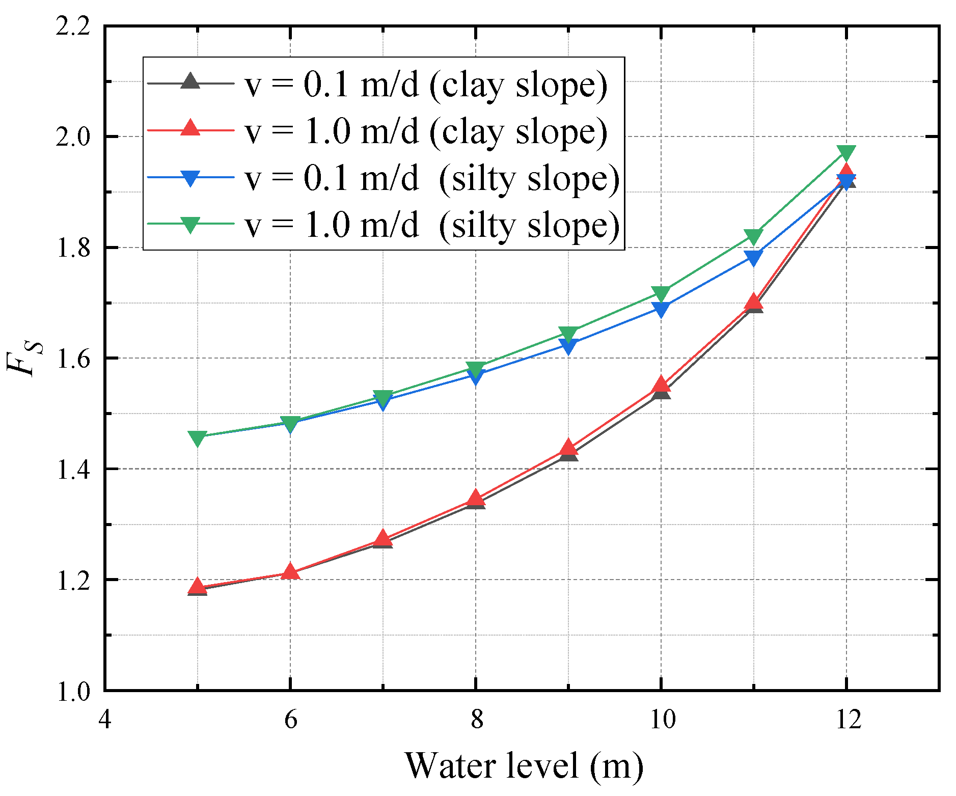
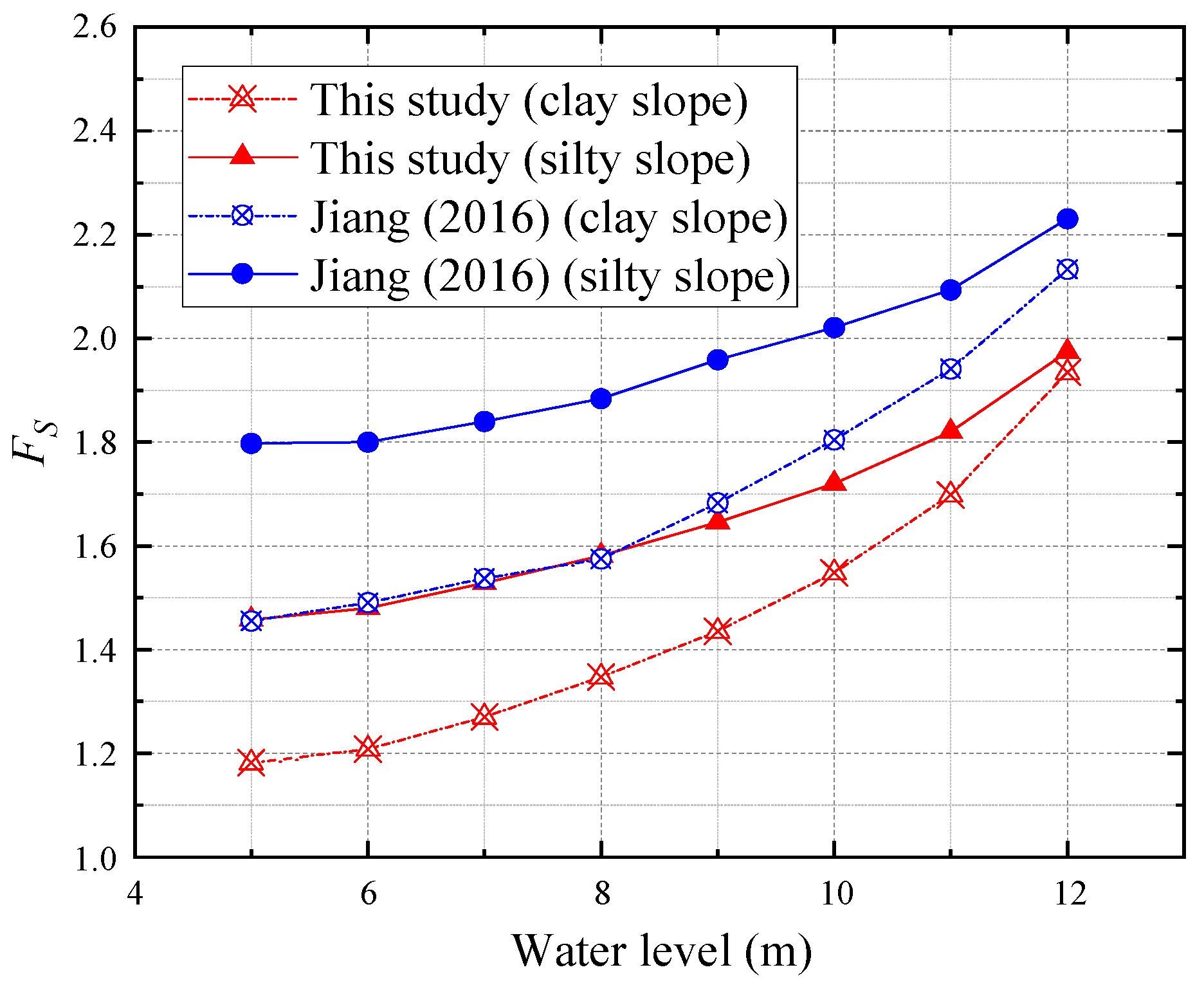
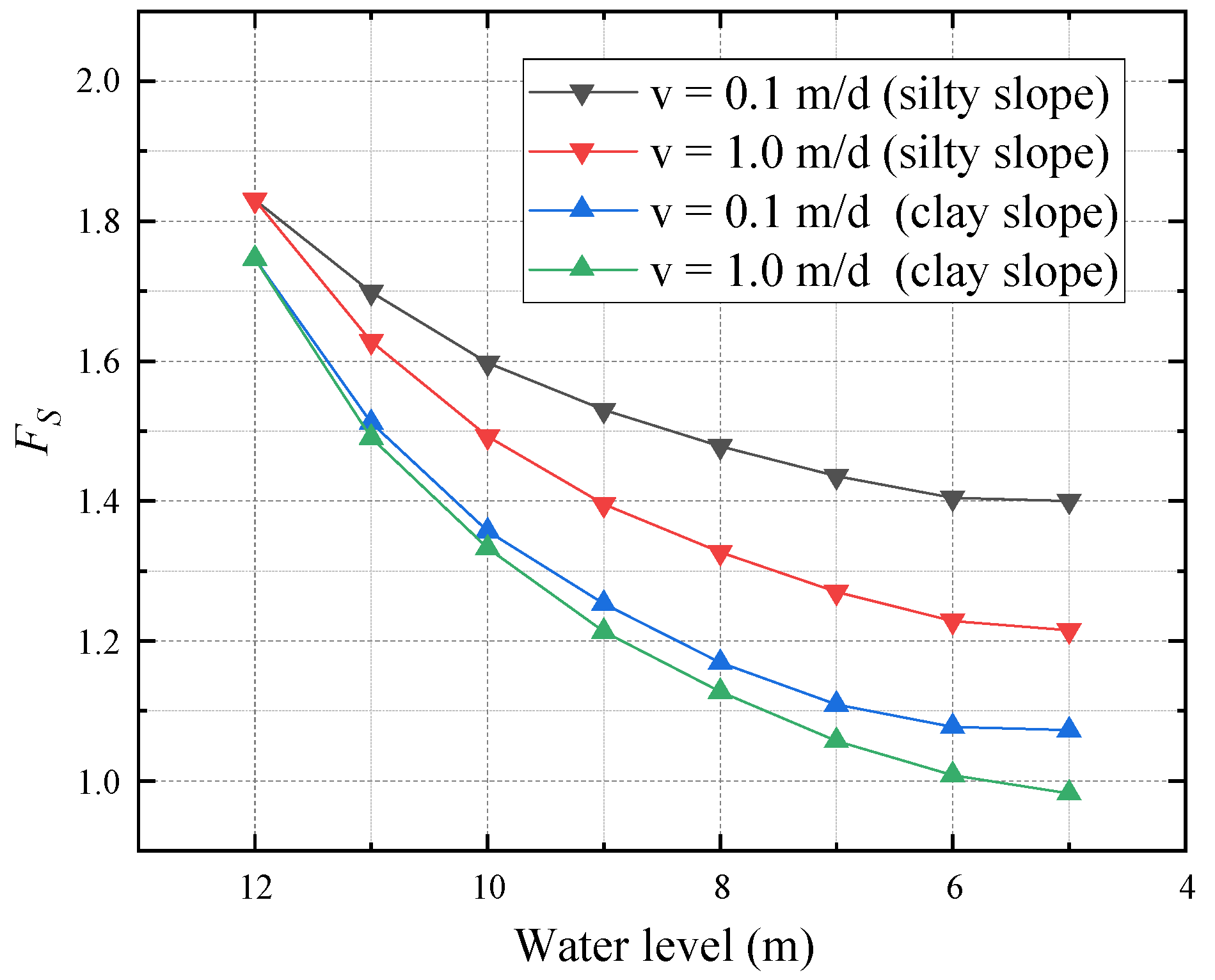
4.3. Effect of Permeability Coefficient

In the actual reservoir slopes, a different permeability coefficient suggests different soil characteristics, such as cohesive strength and internal friction angle. To investigate the pure impact of the permeability coefficient on the reservoir slope stability, we only changed a single variable, the permeability coefficient, in the ideal slope model to discuss the results herein. The model is an inhomogeneous slope with an upper silt layer and limestone bedrock from Shi [47], the soil characteristics are shown in Table 8.
When the reservoir water level drops at a fixed rate of 1.0 m/d and the permeability coefficient of the upper silt varies with 5.79 × 10⁻⁵ cm/s, 5.79 × 10⁻⁴ cm/s, and 5.79 × 10⁻³ cm/s, the corresponding phreatic surfaces are shown in Figure 20.
It could be found that the hysteresis of the phreatic surface significantly varies with different permeability coefficients. When the water level in the reservoir falls, the smaller the permeability coefficient is, the steeper the phreatic surface drops, and the greater the hydraulic gradient, the more pronounced was the hysteresis exhibited by the phreatic surface (higher phreatic surface positions compared to the same external water level). In consideration of the difference in permeability characteristics between upper silt and limestone bedrock, the phreatic surfaces are offset at the interaction between soil layers, especially for those cases with higher permeability coefficients (Figure 20c). In such cases, the critical failure surfaces searched by the IRMO algorithm are shown in Figure 21, and the corresponding minimum FS values are shown in Figure 22.
It could be found that there are no significant differences between the CFSs in the condition of the different permeability coefficients (Figure 21), while the minimum FS of this layered slope decreases by 32.11%, 30.31%, and 28.01%, respectively, as shown in Figure 22. It illustrates that the smaller the permeability coefficient of the slope soils is, the more adverse effect it has on the stability of the slope. When the reservoir water level drops, the groundwater inside the slope seeps outwards, generating dynamic water pressure pointing outwards the slope, which is detrimental to the slope stability. The smaller the permeability coefficient, the more pronounced the hysteresis of the phreatic surfaces inside the slope, the greater the dynamic water pressure, and the longer it exists. Therefore, the smaller permeability coefficient results in a smaller minimum FS for the slope. Additionally, it can be observed that there is a slight increase in minimum FS at the lower water level, which results in the most adverse situation of the slope when the reservoir water level is at 12 m instead of the lowest level. It could be explained that, after the reservoir water level drops over 12 m, the remaining groundwater inside the slope still gradually seeps outward as the lag effects. As the phreatic surfaces gradually flatten out during the descent, the hydraulic gradient decreases, leading to a decrease in the dynamic water pressure. Moreover, the pore water pressure constantly decreases as the groundwater seeps out, the matrix suction gradually increases, and the shear strength of the soil increases. Ultimately, before the reservoir water level drops to its lowest position, the minimum FS slightly rebounds. Therefore, it is necessary to control the dropping rate of the reservoir water level to reduce the slope instability before the lowest water level during reservoir drawdown.

5. Conclusions

By employing the slope stability analysis method based on the IRMO algorithm and rigorous Janbu method considering the seepage effect, this study validated the effectiveness and superiority of the proposed program. Subsequently, it examined the influence of the reservoir water level fluctuation direction, the rate of variation, and the soil permeability coefficient on the stability of the reservoir slope. The following conclusions are obtained:
  • The studies herein demonstrate that both the increase and decrease in the reservoir water level will significantly impact the stability of the reservoir slope. With the rising reservoir water level, the minimum FS of silt slope and clay slope will increase, and the possible slide body will be also be larger. It can be argued that the rising reservoir water level significantly increases the hydrostatic pressure, which is beneficial for stability, compared to the unfavourable seepage force which increases less relatively due to the hysteresis of the seepage field. When the reservoir water level drops, the minimum Fs will decrease significantly. But, with the lower water level, the minimum Fs will decrease slowly and then increase slightly after reaching the most dangerous water level. Due to the relative hysteresis of the seepage changes, the phreatic surface will continue to decrease after reaching the lowest reservoir water level, which leads to a slight increase in the minimum FS of the reservoir slope.
  • In the process of the reservoir water level rising and falling, the fluctuation rate of water level and soil permeability coefficient could influence the reservoir slope stability. With a higher change rate of water level rising or falling and a smaller permeability coefficient, the hysteresis effect of seepage will be more serious, and the corresponding minimum Fs will increase or decrease more rapidly.
  • However, the proposed method in this study did not consider the influence of the matric suction of the saturated–unsaturated area. Compared to the results that consider the matric suction effect in the same slope model, the minimum FS results are higher during the water level rising and lower during the water level falling. This illustrates that the matric suction has a great influence on the stability of the slope. Therefore, it is necessary to figure out the change and effect of matric suction inside the slope in further studies for stability analysis.

Author Contributions

Conceptualisation, L.J. and C.L.; methodology, C.L.; software, C.L. and J.W.; validation, C.L. and J.W.; formal analysis, C.L. and J.W.; investigation, C.L.; resources, C.L.; data curation, C.L. and J.W.; writing—original draft preparation, C.L. and J.W.; writing—review and editing, L.J.; visualisation, J.W.; supervision, L.J.; project administration, L.J. and P.L. All authors have read and agreed to the published version of the manuscript.

Funding

This research received no external funding.

Data Availability Statement

Dataset available upon request from the authors.

Conflicts of Interest

The authors declare no conflicts of interest.

References

  1. Nakamura, H.; Wang, G. Study on landslide in reservior area. Bull. Soil Water Conserv. 1990, 10, 53–64. [Google Scholar] [CrossRef]
  2. Li, X. Stability Analysis of Colluvial Landslide in Relation to Variation of Water Level in Wanzhou District, Three Gorges Reservoir Doctor; China University of Geosciences: Wuhan, China, 2021. [Google Scholar]
  3. Michalowski, R.L.; Nadukuru, S.S. Three-Dimensional Limit Analysis of Slopes with Pore Pressure. J. Geotech. Geoenviron. Eng. 2013, 139, 1604–1610. [Google Scholar] [CrossRef]
  4. Rao, P.; Zhao, L.; Chen, Q.; Nimbalkar, S. Three-dimensional slope stability analysis incorporating coupled effects of pile reinforcement and reservoir drawdown. Int. J. Geomech. 2019, 19, 6019002. [Google Scholar] [CrossRef]
  5. Viratjandr, C.; Michalowski, R.L. Limit analysis of submerged slopes subjected to water drawdown. Can. Geotech. J. 2006, 43, 802–814. [Google Scholar] [CrossRef]
  6. Meng, Q.; Qian, K.; Zhong, L.; Gu, J.; Li, Y.; Fan, K.; Yan, L. Numerical analysis of slope stability under reservoir water level fluctuations using a FEM-LEM-combined method. Geofluids 2020, 2020, 6683311. [Google Scholar] [CrossRef]
  7. Zhou, X.-P.; Wei, X.; Liu, C.; Cheng, H. Three-dimensional stability analysis of bank slopes with reservoir drawdown based on rigorous limit equilibrium method. Int. J. Geomech. 2020, 20, 4020229. [Google Scholar] [CrossRef]
  8. Kafle, L.; Xu, W.-J.; Zeng, S.-Y.; Nagel, T. A numerical investigation of slope stability influenced by the combined effects of reservoir water level fluctuations and precipitation: A case study of the Bianjiazhai landslide in China. Eng. Geol. 2022, 297, 106508. [Google Scholar] [CrossRef]
  9. Sun, L.; Tang, X.; Abdelaziz, A.; Liu, Q.; Grasselli, G. Stability analysis of reservoir slopes under fluctuating water levels using the combined finite-discrete element method. Acta Geotech. 2023, 18, 5403–5426. [Google Scholar] [CrossRef]
  10. Zhang, G.; Lu, G.; Xia, C.; Bai, D.; Liu, T. A Time-Scale Varying Finite Difference Method for Analyzing the Influence of Rainfall and Water Level on the Stability of a Bank Slope. Appl. Sci. Basel 2023, 13, 5268. [Google Scholar] [CrossRef]
  11. Liu, Y.; Zhang, W.; Zhang, L.; Zhu, Z.; Hu, J.; Wei, H. Probabilistic stability analyses of undrained slopes by 3D random fields and finite element methods. Geosci. Front. 2018, 9, 1657–1664. [Google Scholar] [CrossRef]
  12. Wang, M.-Y.; Liu, Y.; Ding, Y.-N.; Yi, B.-L. Probabilistic stability analyses of multi-stage soil slopes by bivariate random fields and finite element methods. Comput. Geotech. 2020, 122, 103529. [Google Scholar] [CrossRef]
  13. Griffiths, D.V. Slope stability analysis by finite elements. Géotechnique 1999, 49, 387–403. [Google Scholar] [CrossRef]
  14. Mandal, A.K.; Li, X.; Shrestha, R. Influence of Water Level Rise on the Bank of Reservoir on Slope Stability: A Case Study of Dagangshan Hydropower Project. Geotech. Geol. Eng. 2019, 37, 5187–5198. [Google Scholar] [CrossRef]
  15. Zhang, W.J.; Zhan, L.T.; Ling, D.S.; Chen, Y.M. Influence of reservoir water level fluctuations on stability of unsaturated soil banks. J. Zhejiang Univ. Eng. Sci. 2006, 40, 1365–1370. [Google Scholar] [CrossRef]
  16. Zhang, X.; Dai, Z. Analysis of slope stability under seepage by using ABAQUS program. Chin. J. Rock Mech. Eng. 2010, 29, 2927–2934. [Google Scholar]
  17. Mao, J.-Z.; Guo, J.; Fu, Y.; Zhang, W.-P.; Ding, Y.-N. Effects of Rapid Water-Level Fluctuations on the Stability of an Unsaturated Reservoir Bank Slope. Adv. Civ. Eng. 2020, 2020, 2360947. [Google Scholar] [CrossRef]
  18. Zheng, Y.; Shi, W.; Kong, W. Calculation of seepage forces and phreatic surface under drawdown conditions. Chin. J. Rock Mech. Eng. 2004, 23, 3203. [Google Scholar] [CrossRef]
  19. Zheng, Y.; Tang, X. Stability analysis of slopes under drawdown condition of reservoirs. Chin. J. Geotech. Eng. 2007, 29, 1115–1121. [Google Scholar] [CrossRef]
  20. Sun, G.; Yang, Y.; Cheng, S.; Zheng, H. Phreatic line calculation and stability analysis of slopes under the combined effect of reservoir water level fluctuations and rainfall. Can. Geotech. J. 2017, 54, 631–645. [Google Scholar] [CrossRef]
  21. Deng, D.; Li, L.; Zhao, L. A new method for analysis of slope stability under steady seepage. Chin. J. Eng. Geol. 2011, 19, 29–36. [Google Scholar] [CrossRef]
  22. Lu, Y.; Chen, X. Solution for stability of soil slopes subjected to seepage of groundwater via simplified Bishop Method. Chin. J. Appl. Mech. 2018, 35, 524–529+687. [Google Scholar] [CrossRef]
  23. Chen, Z.-Y. Random trials used in determining global minimum factors of safety of slopes. Can. Geotech. J. 1992, 29, 225–233. [Google Scholar] [CrossRef]
  24. Li, S.; Shangguan, Z.; Duan, H.; Liu, Y.; Luan, M. Searching for critical failure surface in slope stability analysis by using hybrid genetic algorithm. Geomech. Eng. 2009, 1, 85–96. [Google Scholar] [CrossRef]
  25. Zolfaghari, A.R.; Heath, A.C.; McCombie, P.F. Simple genetic algorithm search for critical non-circular failure surface in slope stability analysis. Comput. Geotech. 2005, 32, 139–152. [Google Scholar] [CrossRef]
  26. Liu, Q.Q.; Li, J.C. Effects of Water Seepage on the Stability of Soil-slopes. Procedia IUTAM 2015, 17, 29–39. [Google Scholar] [CrossRef]
  27. Gao, W. Determination of the Noncircular Critical Slip Surface in Slope Stability Analysis by Meeting Ant Colony Optimization. J. Comput. Civ. Eng. 2016, 30, 06015001. [Google Scholar] [CrossRef]
  28. Kahatadeniya, K.S.; Nanakorn, P.; Neaupane, K.M. Determination of the critical failure surface for slope stability analysis using ant colony optimization. Eng. Geol. 2009, 108, 133–141. [Google Scholar] [CrossRef]
  29. Khajehzadeh, M.; Taha, M.R.; El-Shafie, A.; Eslami, M. Stability assessment of earth slope using modified particle swarm optimization. Chin. J. Inst. Eng. 2014, 37, 79–87. [Google Scholar] [CrossRef]
  30. Shinoda, M.; Miyata, Y. PSO-based stability analysis of unreinforced and reinforced soil slopes using non-circular slip surface. Acta Geotech. 2018, 14, 907–919. [Google Scholar] [CrossRef]
  31. Himanshu, N.; Burman, A. Determination of Critical Failure Surface of Slopes Using Particle Swarm Optimization Technique Considering Seepage and Seismic Loading. Geotech. Geol. Eng. 2018, 37, 1261–1281. [Google Scholar] [CrossRef]
  32. Li, S.J.; Liu, Y.X.; He, X.; Liu, Y.J. Global search algorithm of minimum safety factor for slope stability analysis based on annealing simulation. Chin. J. Rock Mech. Eng. 2003, 22, 236. [Google Scholar] [CrossRef]
  33. Zhang, K.; Xu, Q.; Wang, Y.; A, H. Application of self-adaptive differnetial evolution algorithm in searching for critical slip surface of slope. Rock Soil Mech. 2017, 38, 1503–1509. [Google Scholar] [CrossRef]
  34. Cen, W.J.; Luo, J.R.; Yu, J.S.; Shamin Rahman, M. Slope Stability Analysis Using Genetic Simulated Annealing Algorithm in Conjunction with Finite Element Method. KSCE J. Civ. Eng. 2019, 24, 30–37. [Google Scholar] [CrossRef]
  35. Biniyaz, A.; Azmoon, B.; Liu, Z. Coupled transient saturated–unsaturated seepage and limit equilibrium analysis for slopes: Influence of rapid water level changes. Acta Geotech. 2021, 17, 2139–2156. [Google Scholar] [CrossRef]
  36. Jin, L.X.; Wei, J.J.; Luo, C.W. Slope stability analysis based on improved radial movement optimization considering seepage effect. Alex. Eng. J. 2023, 79, 591–607. [Google Scholar] [CrossRef]
  37. Rahmani, R.; Yusof, R. A new simple, fast and efficient algorithm for global optimization over continuous search-space problems: Radial Movement Optimization. Appl. Mech. Mater. 2014, 248, 287–300. [Google Scholar] [CrossRef]
  38. Pan, Z.F.; Jin, L.X.; Chen, W.S. Improved radial movement optimization algorithm for slope stability analysis. Rock Soil Mech. 2016, 37, 2080–2084. [Google Scholar] [CrossRef]
  39. Jin, L.; Feng, Q.; Pan, Z. Slope Stability Analysis Based on Morgenstern-Price Method and Improved Radial Movement Optimization Algorithm. China J. Highw. Transp. 2018, 31, 39–47. [Google Scholar] [CrossRef]
  40. Jin, L.; Feng, Q. Improved radial movement optimization to determine the critical failure surface for slope stability analysis. Environ. Earth Sci. 2018, 77, 564. [Google Scholar] [CrossRef]
  41. Pham, H.T.V.; Fredlund, D.G. The application of dynamic programming to slope stability analysis. Can. Geotech. J. 2003, 40, 830–847. [Google Scholar] [CrossRef]
  42. Qin, J. Analysis and Improved of Classical Slope Stability Methods in Seepage Soil Mass. Master’s Thesis, Tianjin University, Tianjin, Chiana, 2014. [Google Scholar]
  43. Chen, Y.; Wei, X.; Yuchao, K. Location non-circular critical slip surfaces by particle swarm optimization algorithm. Chin. J. Rock Mech. Eng. 2006, 25, 1443. [Google Scholar] [CrossRef]
  44. Cheng, Y.M.; Li, L.; Chi, S.C. Performance studies on six heuristic global optimization methods in the location of critical slip surface. Comput. Geotech. 2007, 34, 462–484. [Google Scholar] [CrossRef]
  45. Singh, J.; Banka, H.; Verma, A.K. A BBO-based algorithm for slope stability analysis by locating critical failure surface. Neural Comput. Appl. 2018, 31, 6401–6418. [Google Scholar] [CrossRef]
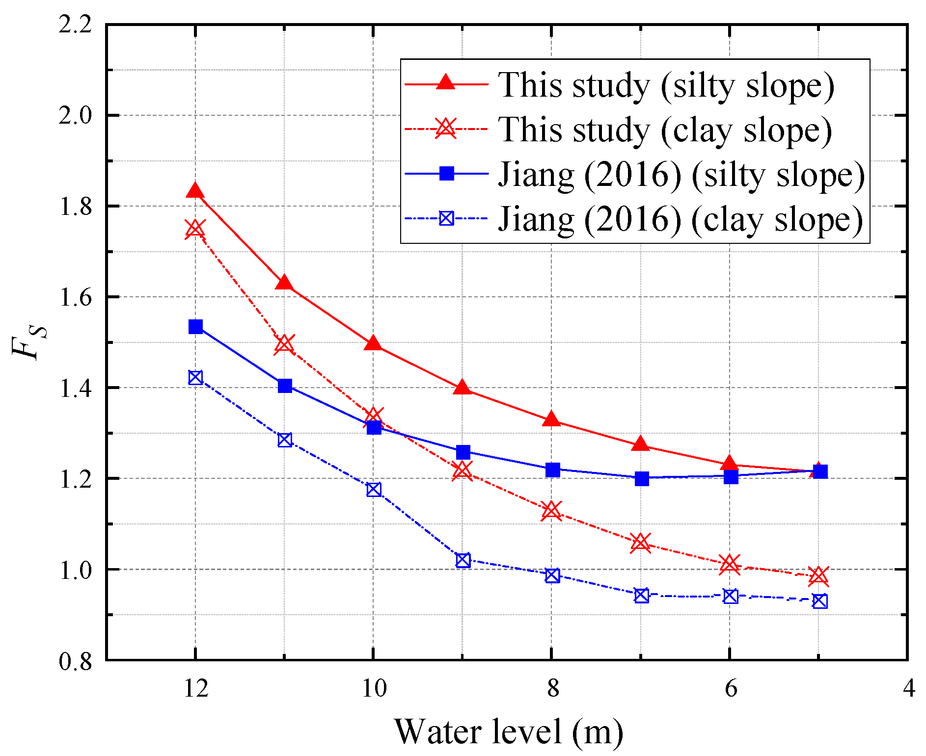
  46. Jiang, Z. Improvement of Critical Slip Field Method of Slope and Development of Its Computing System. Ph.D. Thesis, Hefei University of Technology, Hefei, China, 2016. [Google Scholar]
  47. Shi, D. Numerical Analysis of Binary Structure Slope Stability in Condition of Reservoir Water Level Fluctuation. Master’s Thesis, Kunming University of Science and Technology, Kunming, China, 2020. [Google Scholar]
Figure 1. Statistics of landslide occurrence in Wanzhou District, Three Gorges, since 1950 [2].
Mathematics 12 02055 g001
Figure 2. Simplified seepage field and seepage force.
Mathematics 12 02055 g002
Figure 3. Static equilibrium analysis of water body of slope slice.
Mathematics 12 02055 g003
Figure 4. Force analysis model of a single slice.
Mathematics 12 02055 g004
Figure 5. Non-circular critical failure surface model.
Mathematics 12 02055 g005
Figure 6. Analysis process of IRMO-based reservoir slope stability analysis under the fluctuating water level.
Mathematics 12 02055 g006
Figure 7. Comparison of the critical failure surfaces obtained by various methods [41,42].
Mathematics 12 02055 g007
Figure 8. Phreatic surfaces corresponding to the reservoir water level rising at 0.1 m/d: (a) clay slope; and (b) silt slope.
Mathematics 12 02055 g008
Figure 9. Phreatic surfaces corresponding to the reservoir water level rising at 1.0 m/d: (a) clay slope; and (b) silt slope.
Mathematics 12 02055 g009
Figure 10. Non-circular critical failure surfaces corresponding to the reservoir water level rising at 0.1 m/d: (a) clay slope; and (b) silt slope.
Mathematics 12 02055 g010
Figure 11. Non-circular critical failure surfaces corresponding to reservoir water level rising at 1.0 m/d: (a) clay slope; and (b) silt slope.
Mathematics 12 02055 g011
Figure 12. Minimum FS corresponding to the reservoir water level rising.
Mathematics 12 02055 g012
Figure 13. Comparison of minimum FS (1.0 m/d rising) [46].
Mathematics 12 02055 g013
Figure 14. Phreatic surfaces corresponding to the reservoir water level dropping at 0.1 m/d: (a) clay slope; and (b) silt slope.
Mathematics 12 02055 g014
Figure 15. Phreatic surfaces corresponding to the reservoir water level dropping at 1.0 m/d: (a) clay slope; and (b) silt slope.
Mathematics 12 02055 g015
Figure 16. Non-circular critical failure surfaces corresponding to the reservoir water level dropping at 0.1 m/d: (a) clay slope; and (b) silt slope.
Mathematics 12 02055 g016
Figure 17. Non-circular critical failure surfaces corresponding to the reservoir water level dropping at 1.0 m/d: (a) clay slope; and (b) silt slope.
Mathematics 12 02055 g017
Figure 18. Minimum FS responding to the reservoir water level falling.
Mathematics 12 02055 g018
Figure 19. Comparison of minimum FS (1.0 m/d falling) [46].
Mathematics 12 02055 g019
Figure 20. Phreatic surfaces corresponding to the different permeability coefficients with reservoir water level falling at 1.0 m/d: (a) k = 5.79 × 10⁻⁵ cm/s; (b) k = 5.79 × 10⁻⁴ cm/s; (c) k = 5.79 × 10⁻³ cm/s.
Mathematics 12 02055 g020
Figure 21. Non-circular critical failure surfaces corresponding to different permeability coefficients with the reservoir water level falling at 1.0 m/d: (a) k = 5.79 × 10⁻⁵ cm/s; (b) k = 5.79 × 10⁻⁴ cm/s; and (c) k = 5.79 × 10⁻³ cm/s.
Mathematics 12 02055 g021
Figure 22. Minimum FS corresponding to the different permeability coefficients with the reservoir water level falling at 1.0 m/d.
Mathematics 12 02055 g022
Table 1. Literature review for slope stability analysis considering seepage analysis.
ReferenceLEMsSeepage Analysis MethodsCFSsOptimisation Techniques
Zolfaghari et al. [25]Morgenstern–PricePore–water pressure from distribution steady seepageNon-circularGA
Himanshu et al. [31]BishopPore–water pressure from distribution steady seepageCircularPSO
Biniyaz et al. [35]Simplified BishopTransient pore–water pressure distribution from saturated–unsaturated flowCircularFEM (FEniCS)
Liu et al. [26]SpencerOne-dimensional groundwater flow in the unconfined aquiferNon-circular (spline curve)GA
Jin et al. [36]Rigorous JanbuInfiltration analysis from two-dimensional steady seepageNon-circularIRMO
Table 2. Results comparison of the four slope case studies by different methods.
CasesReferenceOptimisation MethodsLEMsMinimum FSError
Homogeneous slope casePham and Fredlund [41]SLOPE/WMorgenstern–Price1.168−13.8%
SLOPE/WSimplified Bishop1.167−13.7%
Qin [42]FortranFellenius1.070−12.9%
FortranSimplified Bishop1.185−33.5%
FortranRigorous Janbu1.178−32.3%
Jin et al. [36]IRMORigorous Janbu1.007Average in −21.2%
Inhomogeneous slope case with two-layered soilPham and Fredlund [41]SLOPE/WMorgenstern–Price1.485−8.9%
SLOPE/WSimplified Bishop1.483−8.8%
Qin [42]FortranFellenius1.376
1.489
−1.7%
FortranBishop−9.1%
Jin et al. [36]IRMORigorous Janbu1.353Average in −7.1%
Inhomogeneous slope case with a weak inter-layerPham and Fredlund [41]SLOPE/WMorgenstern–Price1.140−7.7%
SLOPE/WSimplified Bishop1.125−10.9%
Chen et al. [43]PSO & FEM-1.053−0.1%
Jin et al. [36]IRMORigorous Janbu1.052Average in −6.2%
Inhomogeneous slope case in four soil layeredZolfaghari et al. [25]GAMorgenstern–Price1.360−10.6%
Cheng et al. [44]SASpencer1.284−5.3%
GASpencer1.232−1.3%
PSOSpencer1.210+0.5%
Tabu searchSpencer1.343−10.4%
ACOSpencer1.449−16.1%
Kahatadeniya et al. [28]ACOMorgenstern–Price1.377−11.7%
Khajehzadeh et al. [29]PSOMorgenstern–Price1.203+1.1%
MPSOMorgenstern–Price1.171+3.8%
Singh et al. [45]BBOBishop1.348−9.8%
BBOFellenius1.226−0.8%
BBOJanbu2.103−42.2%
BBOJanbu corrected2.104−42.2%
Jin et al. [36]IRMORigorous Janbu1.216Average in −11.2%
Table 3. The minimum FS obtained by IRMO, RMO, DE, and PSO for 20 trials.
Optimisation AlgorithmsMinimum FsStandard DeviationAverage CPU Time (ms)
MaximumMinimumAverage
Homogeneous slope case [36,41]IRMO1.00921.00421.00660.0013755.85
RMO1.03021.01161.01730.0048713.90
DE1.07151.03421.05710.0092431.30
PSO1.08901.02931.05940.01962104.05
Inhomogeneous slope case with a weak inter-layer [36,43]IRMO1.07751.04121.06380.0093665.50
RMO1.14971.03411.09320.0249643.20
DE1.19651.10481.13950.0216395.90
PSO1.29781.11381.19620.05052087.60
Table 4. The framework of the Improved Radial Movement Optimisation algorithm.
IRMO Algorithm:
Input:
1.
Set the fitness function: min f(X),
2.
Set algorithm parameters: Population size M, Number of variables N, Generation G,
Initialisation:
3.
Generate the initial population randomly [XM,N]1;
4.
Calculate the initial function value of each particle f(Xi), i = 1, 2, 3, …, M
5.
According to the function values f(Xi), select the initial central particle Center1,
Evolution:
6.
Randomly generate two parameters r1 and r2 between (0, 1), according to the value of r1 and r2, select the evolution method of the next generation:
6-1.
Directly inherit the position information (variables’ value) of excellent particles,
6-2.
Generate new particles according to the position of the central particle Centerk,
7.
Calculate the function value f(Xik+1) of new generation [XM,N]k+1,
8.
According to the function values f(Xik+1) and the position of central particle Centerk, update the central particle Centerk+1,
9.
If the termination conditions, including calculation accuracy condition and generation condition, are not satisfied, repeat processes 6–8,
Output:
10.
Once the termination conditions are satisfied, output the optimal solution and corresponding variables.
Table 5. Tuned parameters of the IRMO algorithm for the following case studies.
Population Size
(M)
Number of Variables
(N)
Generations
(G)
Coefficients
C1C2
IRMO250502500.40.5
Table 6. Comparison of minimum FS obtained by various methods.
ReferenceComputation TechniquesSeepage AnalysisSlope Stability AnalysisCritical Failure SurfaceMinimum FS
Pham and Fredlund [41] FlexPDSDistribution of pore–water pressuresDNYPROG (μ = 0.48)Non-circular1.187
FlexPDSDNYPROG (μ = 0.33)Non-circular1.041
SIGMA/W and SEEP/WEnhanced (μ = 0.48)Circular1.171
SIGMA/W and SEEP/WEnhanced (μ = 0.33)Circular1.132
SLOPE/WMorgenstern–PriceCircular1.168
SLOPE/WSimplified BishopCircular1.167
Qin [42]FortranConsidering seepage forceFelleniusCircular1.070
Simplified BishopCircular1.185
Rigorous JanbuCircular1.178
This studyIRMOWithout considering seepage forceRigorous JanbuNon-circular1.181
Considering seepage forceRigorous JanbuNon-circular1.007
Note: μ is the Poisson’s ratio.
Table 7. Soil properties of slopes in this case.
Soilγ (kN/m3)c (kPa)φ (°)Permeability Coefficient k (m/s)
clay20.210205.4 × 10−7
silty20.25305.4 × 10−6
Table 8. Soil characteristics of slope in case 2.
Soilγ (kN/m3)c (kPa)φ (°)
Upper silt layer201025
Limestone bedrock256742
Disclaimer/Publisher’s Note: The statements, opinions and data contained in all publications are solely those of the individual author(s) and contributor(s) and not of MDPI and/or the editor(s). MDPI and/or the editor(s) disclaim responsibility for any injury to people or property resulting from any ideas, methods, instructions or products referred to in the content.

