
Testing a Class of Piece-Wise CHARN Models with Application to Change-Point Study


Abstract
:1. Introduction
2. Notation and Assumptions
2.1. The Notation
2.2. The Main Assumptions
- (A1)
- and .
- (A2)
- f is differentiable with derivative .
- (A3)
- (A4)
- is differentiable with derivative and is -Lipschitz where
- (A5)
- (A6)
- For any , designates the number of observations between the instants and , such that and , as n tends to .
- (A7)
- For all the sequence is stationary and ergodic on with stationary cumulative distribution function .
- (A8)
- For any , and ,
- (A9)
- , for some positive function defined on .
- (A10)
- For .
- (A11)
- The density function of the first d observations on each interval under converges to its density function under .
- Assumptions (A1)–(A5) are regularity properties required for the density f. They are satisfied at least by the standard Gaussian density function.
- Assumption (A6) allows for the application of the ergodic theorem on each segment . This assumption is very usual in the literature.
- Assumption (A7) ensures the ergodicy and stationarity of the process on each segment . It holds at least for piece-wise stationary and ergodic AR and ARCH models.
- Assumptions (A8)–(A10) are constraints on the function T and its derivatives. They are satisfied by usual models as parametric AR, ARCH, TARCH, and EXPAR models with Gaussian noise.
- Assumption (A11) allows for the simplification of the forms of the likelihoods.
3. The Theoretical Results
3.1. The Parameters Are Known
- [i]
- Under , as ,
- [ii]
- Under , at the level of significance of , the asymptotic power of the test based on iswhere is the -quantile of a standard Gaussian distribution with cumulative distribution function Φ.
- [iii]
- The test based on is locally asymptotically optimal.
3.2. The Parameters Are Unknown
- ()
- The model is identifiable, that is, for , ,
- ()
- The true parameter has a consistent estimator that satisfies the Bahadur representation (see, e.g., [29]), given bywhere
- .
- For any , such that
- and .
- ()
- For any ,
- ()
- For any and , there exists a ball of radius r, such that
- ()
- For and ,
- In the literature, one can find numbers of models with functions satisfying () and ().
- [i]
- Under :
- [ii]
- Under :whereand
3.2.1. The Parameter Is Known
- [i]
- [ii]
- [i]
- Under , as , .
- [ii]
- Under at the level of significance , the asymptotic power of the test based on the statistic is , where is the -quantile of the standard Gaussian distribution with cumulative distribution function Φ.
- [iii]
- The test based on the statistic is locally asymptotically optimal.
3.2.2. The Parameter Is Unknown
- ()
- For any , , forfor some positive function defined on
- ()
- For , and ,
- ()
- .
- [i]
- Under , as , .
- [ii]
- Under at the level of significance , the asymptotic power of the test based on the statisticis , where is the -quantile of the standard Gaussian distribution with cumulative distribution function Φ.
- [iii]
- The test based on the statistic is locally asymptotically optimal.
4. Application to Detection of Change Points and Their Location Estimation
- Location 1:
- (A1): Take any t between 1 and so that there is a large number of indices before and after t (for example ).
- Adjust Model (1) to with a potential change located at the time index t, and apply the testing procedure studied.
- If
- Put and go to Location 2 (first change location estimated)
- Else
- Carry out and go to (A1).
- Location 2:
- Consider the next h observations to :
- Put and conduct the following:
- (A2): Take any t between and so that there is a large number of indices before and after t.
- Adjust Model (1) to with a potential change located at the time index t and apply the testing procedure studied.
- If ,
- Put and go to Location 3 (second change location estimated)
- Else
- Carry out and go to (A2).
- Location i:
- Let be the change location at step i-1
- Put and perform
- (Ai): Take any t between and so that there is a large number of indices before and after t.
- Adjust Model (1) to with a potential change located at the time index t and apply the testing procedure studied
- If ,
- Put , and go to Location i (ith change location estimated)
- Else
- Carry out and go to (Ai).
5. Simulation Experiment
5.1. Simulation Methodology
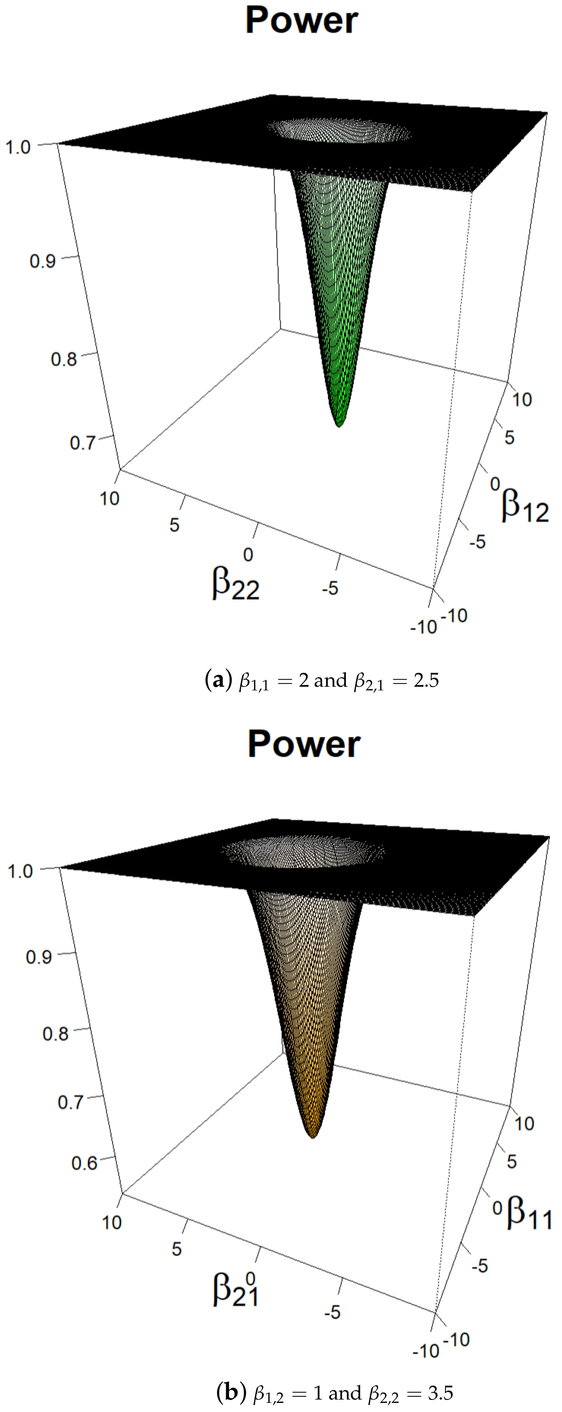
5.2. Power Study for Given Break Locations
5.2.1. and f Are Known
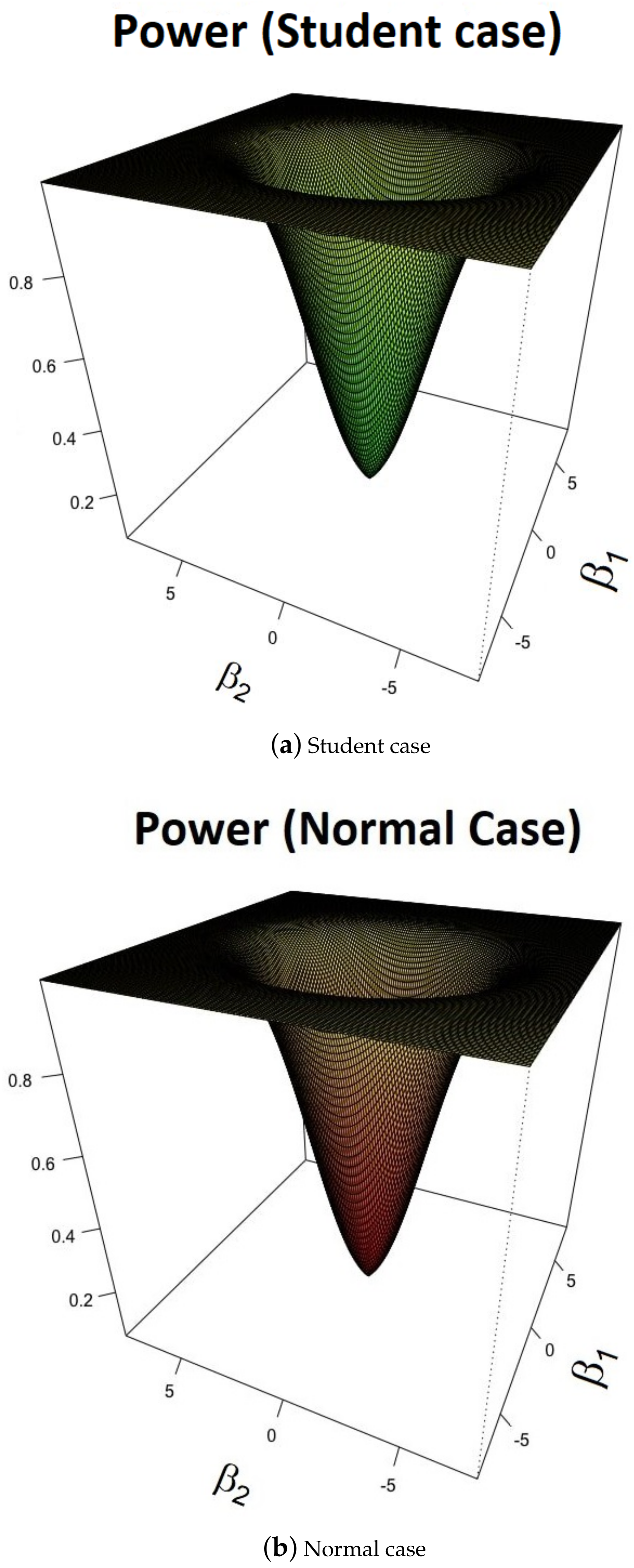
5.2.2. and f Are Unknown
- 1.
- for any (positivity).
- 2.
- (density).
- 3.
- (by symmetry).
5.3. Detection of Change Points and Estimation of Their Locations
5.3.1. No Break
5.3.2. Case of One Single Break
5.4. Case of Three Breaks ()
5.4.1. AR(1) Models
5.4.2. AR(1)-ARCH(1) Models
5.4.3. Conclusions
5.5. Comparison with [27]
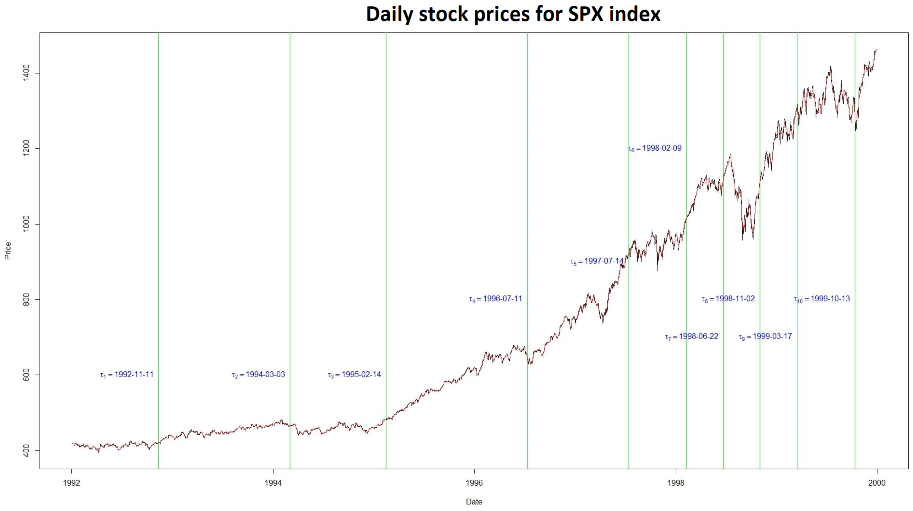
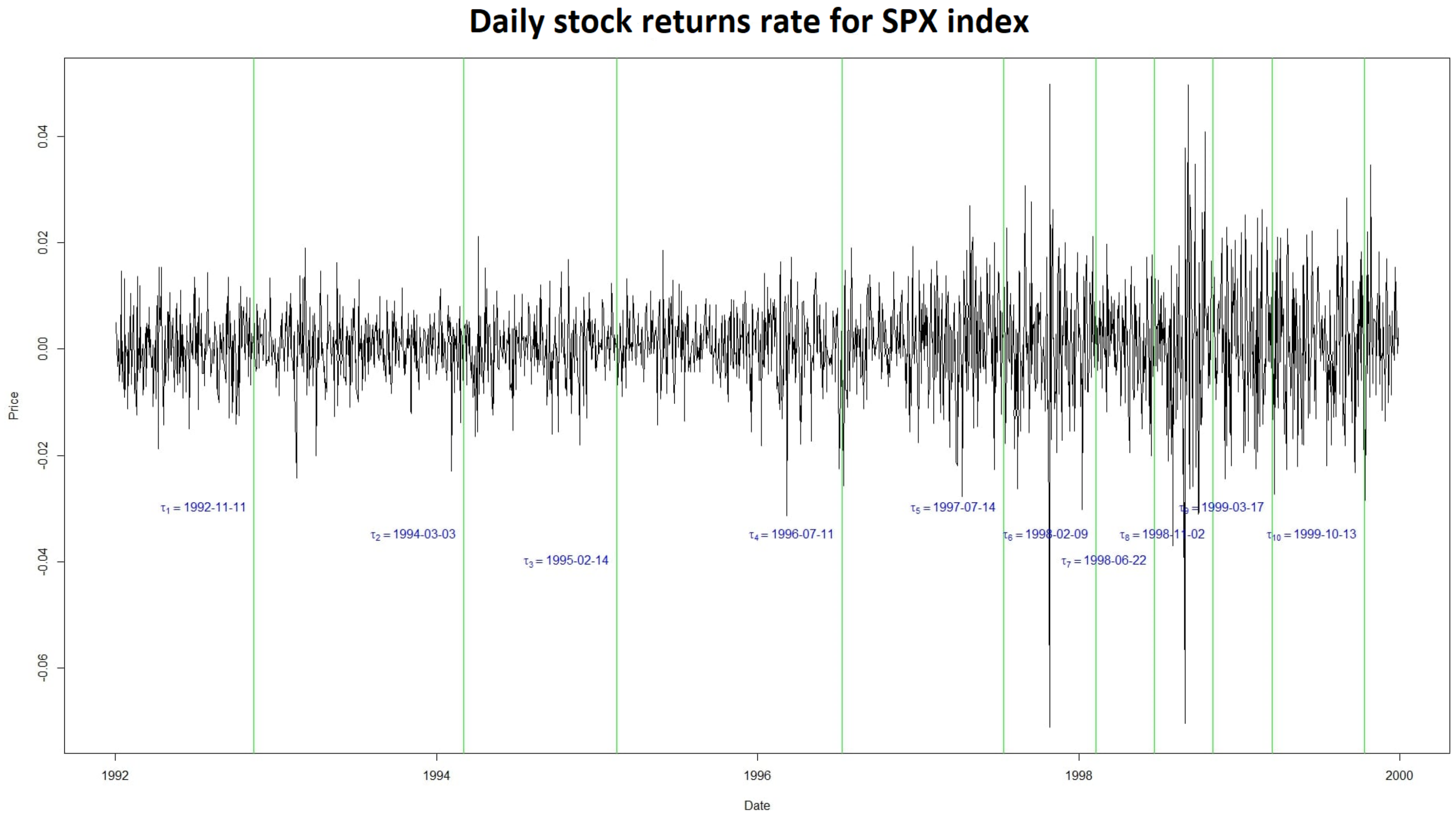
5.6. Application to Real Data
6. Conclusions
Author Contributions
Funding
Data Availability Statement
Conflicts of Interest
Appendix A. Proofs
Appendix A.1. Proof of Theorem 1
- and for ,
- where is a null matrix and for any
- where, for ,
Appendix A.2. Proof of Corollary 1
Appendix A.3. Proof of Theorem 2
Appendix A.4. Proof of Proposition 1
Appendix A.4.1. Proof of [i]
Appendix A.4.2. Proof of [ii]
Appendix A.5. Proof of Proposition 2
Appendix A.5.1. Proof of [i]
Appendix A.5.2. Proof of [ii]
Appendix A.6. Proof of Theorem 3
Appendix A.6.1. Proof of [i]
Appendix A.6.2. Proof of [ii] and [iii]
Appendix A.7. Proof of Proposition 3
Appendix A.8. Proof of Theorem 4
Appendix A.8.1. Proof of [i]
Appendix A.8.2. Proof of [ii] and [iii]
References
- Härdle, W.; Tsybakov, A.; Yang, L. Nonparametric vector autoregression. J. Stat. Plan. Inference 1998, 68, 221–245. [Google Scholar] [CrossRef]
- Chen, G.; Gan, M.; Chen, G. Generalized exponential autoregressive models for nonlinear time series: Stationarity, estimation and applications. Inf. Sci. 2018, 438, 46–57. [Google Scholar] [CrossRef]
- Yau, Y.C.; Zhao, Z. The asymptotic behavior of the likelihood ratio statistic for testing a shift in mean in a sequence of independent normal variates. J. R. Statist. Soc. 2016, 48, 895–916. [Google Scholar] [CrossRef]
- Ngatchou-Wandji, J.; Ltaifa, M. Detecting weak changes in the mean of a class of nonlinear heteroscedastic models. Commun. Stat. Simul. Comput. 2023, 1–33. [Google Scholar] [CrossRef]
- Csörgő, M.; Horváth, L.; Szyszkowicz, B. Integral tests for suprema of kiefer processes with application. Stat. Risk Model. 1997, 15, 365–378. [Google Scholar] [CrossRef]
- MacNeill, I.B. Tests for change of parameter at unknown times and distributions of some related functionals on brownian motion. Ann. Stat. 1974, 2, 950–962. [Google Scholar] [CrossRef]
- Chernoff, H.; Zacks, S. Estimating the current mean of a normal distribution which is subjected to changes in time. Ann. Math. Stat. 1964, 35, 999–1018. [Google Scholar] [CrossRef]
- Davis, R.A.; Huang, D.; Yao, Y.-C. Testing for a change in the parameter values and order of an autoregressive model. Ann. Stat. 1995, 23, 282–304. [Google Scholar] [CrossRef]
- Vogelsang, T.J. Wald-type tests for detecting breaks in the trend function of a dynamic time series. Econom. Theory 1997, 13, 818–848. [Google Scholar] [CrossRef]
- Andrews, D.W.; Ploberger, W. Optimal tests when a nuisance parameter is present only under the alternative. Econom. J. Econom. Soc. 1994, 62, 1383–1414. [Google Scholar] [CrossRef]
- Andrews, D.W. Tests for parameter instability and structural change with unknown change point. Econom. J. Econom. Soc. 1993, 61, 821–856. [Google Scholar] [CrossRef]
- Lavielle, M.; Lebarbier, E. An application of MCMC methods for the multiple change-points problem. Signal Process. 2001, 81, 39–53. [Google Scholar] [CrossRef]
- Lebarbier, É. Detecting multiple change-points in the mean of Gaussian process by model selection. Signal Process. 2005, 85, 717–736. [Google Scholar] [CrossRef]
- Davis, R.A.; Lee, T.C.; Rodriguez-Yam, G.A. Break detection for a class of nonlinear time series models. J. Time Ser. Anal. 2008, 29, 834–867. [Google Scholar] [CrossRef]
- Fotopoulos, S.B.; Jandhyala, V.K.; Tan, L. Asymptotic study of the change-point mle in multivariate gaussian families under contiguous alternatives. J. Stat. Plan. Inference 2009, 139, 1190–1202. [Google Scholar] [CrossRef]
- Huh, J. Detection of a change point based on local-likelihood. J. Multivar. Anal. 2010, 101, 1681–1700. [Google Scholar] [CrossRef]
- Jarušková, D. Asymptotic behaviour of a test statistic for detection of change in mean of vectors. J. Stat. Plan. Inference 2010, 140, 616–625. [Google Scholar] [CrossRef]
- Piterbarg, V.I. High Derivations for Multidimensional Stationary Gaussian Process with Independent Components. In Stability Problems for Stochastic Models; De Gruyter: Berlin, Germany; Boston, MA, USA, 1994; pp. 197–210. [Google Scholar]
- Chen, K.; Cohen, A.; Sackrowitz, H. Consistent multiple testing for change points. J. Multivar. Anal. 2011, 102, 1339–1343. [Google Scholar] [CrossRef]
- Vostrikova, L.Y. Detecting “disorder” in multidimensional random processes. In Doklady Akademii Nauk; Russian Academy of Sciences: Moscow, Russia, 1981; Volume 259, pp. 270–274. [Google Scholar]
- Cohen, A.; Sackrowitz, H.B.; Xu, M. A new multiple testing method in the dependent case. Ann. Stat. 2009, 37, 1518–1544. [Google Scholar] [CrossRef]
- Prášková, Z.; Chochola, O. M-procedures for detection of a change under weak dependence. J. Stat. Plan. Inference 2014, 149, 60–76. [Google Scholar] [CrossRef]
- Dupuis, D.; Sun, Y.; Wang, H.J. Detecting Change-Points in Extremes; International Press of Boston: Boston, MA, USA, 2015. [Google Scholar]
- Badagián, A.L.; Kaiser, R.; Peña, D. Time series segmentation procedures to detect, locate and estimate change-points. In Empirical Economic and Financial Research; Springer: Berlin/Heidelberg, Germany, 2015; pp. 45–59. [Google Scholar]
- Yau, C.Y.; Zhao, Z. Inference for multiple change points in time series via likelihood ratio scan statistics. J. R. Stat. Soc. Ser. (Stat. Methodol.) 2016, 78, 895–916. [Google Scholar] [CrossRef]
- Ruggieri, E.; Antonellis, M. An exact approach to bayesian sequential change-point detection. Comput. Stat. Data Anal. 2016, 97, 71–86. [Google Scholar] [CrossRef]
- Horváth, L.; Miller, C.; Rice, G. A new class of change point test statistics of Rényi type. J. Bus. Econ. Stat. 2020, 38, 570–579. [Google Scholar] [CrossRef]
- Ltaifa, M. Tests Optimaux pour Détecter les Signaux Faibles dans les Séries Chronologiques. Ph.D. Thesis, Université de Lorraine, Nancy, France, Université de Sousse, Sousse, Tunisia, 2021. [Google Scholar]
- Bahadur, R.R.; Rao, R.R. On deviations of the sample mean. Ann. Math. Stat. 1960, 31, 1015–1027. [Google Scholar] [CrossRef]
- Parzen, E. On estimation of a probability density function and mode. Ann. Math. Stat. 1962, 33, 1065–1076. [Google Scholar] [CrossRef]
- Hall, P.; Heyde, C.C. Martingale Limit Theory and Its Application; Academic Press: Cambridge, MA, USA, 2014. [Google Scholar]
- Le Cam, L. The central limit theorem around 1935. Stat. Sci. 1986, 1, 78–91. [Google Scholar]
- Droesbeke and Fine, J.-J. Inférence Non Paramétrique: Les Statistiques de Rangs; Éditions de l’Université de Bruxelles: Bruxelles, Belgium; Éditions Ellipses: Paris, France, 1996. [Google Scholar]
- Ngatchou-Wandji, J. Estimation in a class of nonlinear heteroscedastic time series models. Electron. J. Stat. 2008, 2, 40–62. [Google Scholar] [CrossRef]
- Ngatchou-Wandji, J. Checking nonlinear heteroscedastic time series models. J. Stat. Plan. Inference 2005, 133, 33–68. [Google Scholar] [CrossRef]
- Salman, Y. Testing a Class of Time-Varying Coefficients CHARN Models with Application to Change-Point Study. Ph.D. Thesis, Lorraine University, Nancy, France, Lebanese University, Beirut, Lebanese, 2022. [Google Scholar]


| 80 | 78 (4.32) | 81 (1.41) | 82 (4.01) | 80 (0.654) | 80 (0.34) |
| 100 | 99 (6.96) | 99 (4.67) | 102 (3.34) | 101 (1.23) | 100 (0.54) |
| 120 | 122 (5.12) | 121 (2.32) | 119 (2.45) | 120 (0.23) | 121 (1.23) |
| 140 | 143 (10.24) | 142 (2.22) | 141 (2.35) | 140 (0.22) | 141 (1.12) |
| 160 | 164 (11.65) | 164 (4.43) | 162 (2.23) | 161 (1.32) | 161 (1.12) |
| 185 | 188 (8.21) | 189 (5.32) | 190 (6.33) | 190 (7.43) | 189 (8.23) |
and | |
|---|---|
| (93,193,277) (5.78) | |
| (93,194,278) (9.87) | |
| (92,193,277) (8.99) |
and | |
|---|---|
| (93,193,277) (9.43) | |
| (93,194,278) (10.64) | |
| (92,193,277) (6.10) |
| Our method | 83 | 81 | 82 | 80 | 80 |
| SCUSUM | 95 | 99 | 86 | 122 | 99 |
| Our method | 122 | 121 | 121 | 120 | 121 |
| SCUSUM | 110 | 114 | 105 | 125 | 122 |
| Our method | 189 | 188 | 186 | 186 | 185 |
| SCUSUM | 105 | 103 | 122 | 114 | 101 |
Disclaimer/Publisher’s Note: The statements, opinions and data contained in all publications are solely those of the individual author(s) and contributor(s) and not of MDPI and/or the editor(s). MDPI and/or the editor(s) disclaim responsibility for any injury to people or property resulting from any ideas, methods, instructions or products referred to in the content. |
© 2024 by the authors. Licensee MDPI, Basel, Switzerland. This article is an open access article distributed under the terms and conditions of the Creative Commons Attribution (CC BY) license (https://creativecommons.org/licenses/by/4.0/).
Share and Cite
Salman, Y.; Ngatchou-Wandji, J.; Khraibani, Z. Testing a Class of Piece-Wise CHARN Models with Application to Change-Point Study. Mathematics 2024, 12, 2092. https://doi.org/10.3390/math12132092
Salman Y, Ngatchou-Wandji J, Khraibani Z. Testing a Class of Piece-Wise CHARN Models with Application to Change-Point Study. Mathematics. 2024; 12(13):2092. https://doi.org/10.3390/math12132092
Chicago/Turabian StyleSalman, Youssef, Joseph Ngatchou-Wandji, and Zaher Khraibani. 2024. "Testing a Class of Piece-Wise CHARN Models with Application to Change-Point Study" Mathematics 12, no. 13: 2092. https://doi.org/10.3390/math12132092