
Approximation of the Interactions of Rarefaction Waves by the Wave Front Tracking Method

Department of Agricultural Engineering, Faculty of Agriculture, University of Novi Sad, 21000 Novi Sad, Serbia
Mathematics 2024, 12(13), 2099; https://doi.org/10.3390/math12132099
Submission received: 27 April 2024
/
Revised: 3 June 2024
/
Accepted: 27 June 2024
/
Published: 4 July 2024
(This article belongs to the Special Issue Computational Mathematics: Advanced Methods and Applications)
Abstract
:The interaction of two simple delta shock waves for a pressureless gas dynamic system is considered. The result of the interaction is a delta shock wave with constant speed. This interaction is approximated by letting the perturbed parameter in the Euler equations for isentropic fluids go to zero. Each delta shock wave is approximated by two shock waves of the first and second family when the perturbed parameter goes to zero. These shock waves are solutions of two Riemann problems at time . The solution of the Riemann problem for can also contain rarefaction waves. If the perturbed parameter approaches 0, the strength of the rarefaction waves increases and the number of interactions of the rarefaction waves increases, as well. When two split rarefaction waves interact, the number of Riemann problems to be solved is , where is the number of ith rarefaction waves. The main topic of this paper is to develop an algorithm that reduces the number of these Riemann problems. The algorithm is based on the determination of the intermediate states that make the Rankine–Hugoniot deficit small. The approximated wave front tracking algorithm was used for the numerical verification of these interactions. The theoretical background was the concept of the shadow wave solution.
Keywords:
pressureless gas dynamics; delta shock waves; wave front tracking method; rarefaction wave interactions approximationMSC:
35L65; 35Q35; 76N151. Introduction
Fluid dynamics problems contain conservation laws. Theoretical background can be found in [1,2]. The author in [2] introduced the linear theory, the reaction–diffusion equations, the shock wave theory, and the Conley index. In addition, the properties and simple one-dimensional wave equation, Holmgren’s theorem, distribution theory, eliptic and parabolic PDE, shock wave theory, and weak solutions have been considered. The book [1] contains nonlinear equations, quasilinear systems, hyperbolic systems, and the theory of characteristics. In addition, Riemann invariants and simple waves were generalized with the theory of one-dimensional gas motion. Shock waves and weak solutions were introduced. Discontinuous solutions (shocks) were treated in a very general context. A detailed analysis of shallow water waves was also given.
The analysis of the conservation laws can be found in the books [3,4]. They contain the classical theory of semilinear and quasilinear systems and describe the method of characteristics for nonlinear scalar equations. Weak solutions, basic definitions, and various conditions for the admissibility of entropy were given. In addition, the concepts of genuinely nonlinear and linear degenerate characteristics were introduced. The authors constructed the standard self-similar solution of the Riemann problem with centered rarefaction, shocks, and contact discontinuity waves. Wave front tracking algorithms were chosen to construct the global solutions of a scalar conservation law. The Cauchy problem for systems of conservation laws with a detailed description of the front-tracking algorithm was also presented with various applications.
In everyday life, humans face shock waves and rarefaction largely in their surroundings. It is therefore necessary to know the behavior of these waves in order to protect oneself from destructive effects. The propagation of shock and rarefaction waves in various dynamics from solving nonlinear hyperbolic inviscid Burgers equation numerically was observed in [5]. Burgers’ equation is explained as a mathematical model for turbulent flow. In recent years, the Burgers equation continued to draw the attention of researchers. It is used as a model to test several numerical methods since it includes a convection term and a viscosity term . As , Burgers equation becomes a hyperbolic equation, called the inviscid Burgers equation, . The authors used the method of characteristics to find the exact solution of the inviscid Burgers equation. The first-order explicit upwind scheme and second-order Lax–Wendroff scheme were used to solve this equation to improve the understanding of numerical diffusion (smearing) and oscillations that can occur when using such schemes. Numerical solutions were investigated for different initial conditions, and the shock and rarefaction waves were studied for the Riemann problem.
A Cauchy problem for hyperbolic conservation laws has two problems. The first is that the solution does not remain continuous in finite time. The second problem is the choice of an admissible solution among several weak solutions. A unique solution to the Cauchy problem is obtained by introducing terms such as admissible wave, physically irrelevant solution, and so on. The admissibility of the weak solution and the complete theoretical basis of the conservation laws are given by Lax [6].
A Cauchy problem (initial value problem) with piecewise constant initial data is called a Riemann problem. For the Euler equations of gas dynamics, one can find a detailed construction of the solution of the Riemann problem in [7,8]. There are many papers in which one can find examples of systems that do not have a classical solution to the Riemann problem. Most of these solutions are delta waves (see [9,10,11]) or singular shock waves (see [12,13]), and they can be considered as special cases of a new type of solution—shadow waves (hereafter referred to as SDW [14]). There are several conditions under which the authors search for a solution for these systems. Here, overcompressibility was a criterion for the admissibility of the wave. A special problem is when the interaction involves singular solutions.
The wave front tracking (WFT) method was generalized by Bressan [15] and Risebro [16]. There was no restriction on the number of generalized equations for genuinely nonlinear systems. In Bressan’s algorithm, a non-physical wave was proposed in the approximate Riemannian solution, whereas Risebro had the idea that the waves merge into one of the two main waves involved in the interaction.
Solving conservation laws with the help of numerical tools is described in [4,17,18]. For example, Glimm’s difference scheme and the WFT method can be used to solve problems in fluid dynamics (see [19,20,21]).
In this paper, the numerical verification of two simple SDW interactions is performed using the WFT method. The algorithms presented by Asakura [22] and Bressan [3] are used. The original problem was modified by introducing the perturbation. Some properties of SDW are exploited to check the relevance of the obtained numerical solution. The specific object of this research is to create the algorithm for approximating the interaction of rarefaction waves to reduce the computational time. Numerical examples showed that, after application of new algorithm, the accuracy remained acceptable while the runtime was drastically reduced.
2. The Pressureless Gas Dynamics Model
The system of hyperbolic PDEs governing the motion of a compressible gas in the absence of viscosity is considered in this manuscript. These consist of conservation laws for mass and momentum. Together they are referred to as the compressible Euler equations or, simply, the Euler equations. The one-dimensional Euler small pressure gas dynamics system is
where is the density, u is the velocity, is a small parameter, and is a parameter, also. Here, is the pressure and moment.
As stated in [9], a solution to the Riemann problem for (1) converges to the generalized solution to the weakly hyperbolic system
with the same initial data as . In the literature, the system (2) can be found as the pressureless gas dynamics model (PGD model [23]). Having the initial data
it is well known that there is no classical solution to the Riemann problem (2,3) if . To be more precise, any two-shock Riemann solution to the Euler equations for isentropic fluids (1) tends to a -shock solution (4), viewed as a distribution,
to the Euler equations for pressureless fluids (2) as the pressure vanishes. Here, with (see [24]).
Nishida and Smoller ([20]) showed that a global weak solution exists for (1,3) and a bounded total variation on each line , provided that times the total variation of the initial data was sufficiently small. If one replaces from [20,22] with , an exact calculation shows that the strength of the wave is now limited by instead of [24]. This allows us to take the initial data with large total variation and set after solving (1).
The interaction problem of the delta shock for the pressureless system was solved in [14,24]. The authors used the SDW solution concept. The result of the interaction of two simple delta shocks is a delta shock with constant speed. Here, the limit of numerical WFT results when the small pressure term vanishes was compared with the SDW solution concept.
Now we present two ideas. The first one is the following: for small enough, two Riemann problems (1,3) are set such that each solution consists of shock waves of the first and second family (this approximates the interaction of two delta shock waves). Next, we apply the WFT method for each and let . The solution results when there are no further interactions. The second idea is to use the SDW solution concept. Finally, a limit for a numerical WFT is obtained when the small pressure term vanishes and the SDW solution has been compared. The one-dimensional Euler gas dynamics system with low pressure (1) was used to approximate the unpressurized gas dynamics model (2) as , i.e., as . The delta shock wave as a solution of (2) was approximated by two shock waves of the first and second family, which are the solutions (together with the rarefaction waves) of the Riemann problem for (1).
Elementary Waves
As in [20], from now on, we choose . Throughout the whole paper [20], authors set to be a small positive constant. Here, is not a constant since we let . To prevent a misunderstanding, note that denotes exponent. The eigenvalues of system (1) are and , and the corresponding eigenvectors are and . The rarefaction curves of (1) through the point are
The shock curves of (1) through the point are
Shock and rarefaction curves are presented in Figure 1.
The Riemann problem for (1) with initial data (3) was solved by Riemann [25]. A detailed explanation of the wave front tracking algorithm can be found in [24]. We will use the following convention: , independent of , denotes the maximum of the constants and from Theorems 2.4 and 2.5 in [24], respectively. As in [24] (Lemma 2.7), is a constant, also independent of .
Theorem 1
A detailed explanation of the modified wave front tracking algorithm can be found in [3,24] and will be omitted here. The following parameters are used for the construction of the modified WFT algorithm:
- —a fixed speed of a non-physical wave,
- —a constant that controls rarefaction waves strength;
- —a number determining which type of Riemann solver is going to be used (accurate or approximative).
3. SDW Solutions to the Pressureless Gas Dynamics Model
The solution concept was taken from [14,24] (somewhat simplified). Its consistency with the numerical WFT results from Theorem 1 by letting is given in [24]. We take a conservation law system (2).
Definition 1
([14,24]). Vector valued function of the form
is called a constant SDW (Figure 2). Further, is called the strength, and c is called the speed of the SDW. The SDW central line is given by , and and are called the external SDW lines. The values and are called the shifts, and and are called the intermediate states of a given SDW. Here, , and and are smooth functions equal zero at with growth order less or equal to ε. If , then SDW is called simple.
Assumption 1
Definition 2
([14]). Delta shock is SDW associated with a δ distribution, with all minor components having finite limits as .
The solution to system (2) is given in the following theorem.
Theorem 2
Now, we give the conditions when the interaction of two simple SDW gives a constant SDW. Let us assume that two simple SDW solutions for (2) interact:
and
where and . Then, as in Figure 3, is the interaction point of external SDW lines and , i.e., and . For , a distributional limit of solution is a sum of a classical piecewise constant function and a delta function supported by the interaction point. Therefore, it is natural to ask ourselves a question: When does the interaction produces a shadow wave solution for ?
Assumption 2
Assumption 3
These two assumptions were analyzed in [14,24]. Let be non-negative real numbers for small enough. Using Lemma 3.2 from [24], it can be concluded that the function
is actually an SDW solution if holds.
Define
The anticipated solution is obtained by gluing the solution before the interaction (for , Figure 3) with the one defined by (7) for :
Based on Assumption 3, there exists such that
Now, following expression (9), the speed of the SDW after the interaction can be expressed as
The condition when the interaction of two simple SDW gives a constant SDW is ([24])
4. Algorithm of a New Concept of Rarefaction Wave Interactions Approximation
In the general case, the solution of Riemann problem (1,3) may contain rarefaction waves as well as shock waves. The expression denotes the rarefaction curve of the ith family, where . Let the curve start from and from . Based on (5), there exists , such that
and
Suppose that connects state from the left and state from the right, i.e., there exists such that . Similarly, let join state from the left and state from the right. As in [3], let , be the small given constants. Consider the integers
where stands for the largest integer . For , , we define the intermediate states and characteristics as follows:
Applying (13) (for ) on (12), we have and
Applying (13) (for ) on (11), we have and
For , ,
and
For , (14) yields
and then
holds. Similarly, for , (15) yields
and then
holds. Expressions (16,17) will be useful later.
Now, the main idea is to use intermediate states and characteristics of as we defined in (13). For , we define new intermediate states and characteristics as follows (see Figure 4):
- Find the intersection point of the two half-lines and , solving the systemWe mark the solution as .
- Solving the systemwe find the intersection between and . Let us denote the solution of this system as .
- Choose to make the RH deficit as small as possible for . To be more precise, after is chosen, we check ifholds for . If it does not hold, we choose and check again, and so on. This stops after steps, even if the inequalities are not satisfied, and we accept new time . Here,holds, based on (17).
- Now, for each we do the following. Find the intersection between and , solving the systemWe denote the solution as . Then, choose to make the RH deficit as small as possible for . After is chosen, we check ifholds. If it does not hold, we choose or ,…until the upper inequalities are satisfied. If it is not a case, then after steps, we accept new time . Here,
- The half-lines that we keep during WFT approximation are , , .
Let us repeat the above procedure, but now we use intermediate states and characteristics of as we defined in (13). For , we define new intermediate states and characteristics as follows (see Figure 5):
- Find the intersection point of the two half-lines and , solving the systemWe mark the solution as .
- Solving the systemwe find the intersection between and . Let us denote the solution of this system as .
- Choose to make the RH deficit as small as possible for . To be more precise, after is chosen, we check ifholds for . If it does not hold, we choose and check again, and so on. This stops after steps, even if the inequalities are not satisfied, and we accept new time . Here,holds, based on (16).
- Now, for each we do the following. Find the intersection between and , solving the systemWe denote the solution as . Then, choose to make the RH deficit as small as possible for . To be more precise, after is chosen, we check ifholds. If it does not hold, we choose or ,…until the upper inequalities are satisfied. If it is not a case, then after steps, we accept new time . Here,
5. Numerical Results
All numerical results were obtained using Mathematica 12.3 software ([26]). The consistency of the theoretical and numerical approaches will are shown. The algorithm of the rarefaction wave interactions approximation are applied in Examples 4 and 5. Let us consider (1) with the initial data
where , . For small enough (see [9]), there exist and , such that:
- and are connected by an 1-shock;
- and are connected by a 2-shock;
- and are connected by an 1-shock;
- and are connected by a 2-shock.
In order to verify two simple delta shock interactions, the WFT algorithm was used to obtain the numerical solutions. The assumption is that can be connected to by a simple SDW; must be chosen such that condition (10) is fulfilled. The result of the interaction is a single SDW with a constant speed.
In the following two examples, (1,18) is considered with , , , , and . Two SDWs will interact at the point . A single constant SDW as a solution to the interaction problem will exist for . After the interaction, the correct speed of the resulting wave equals , obtained from (10). Here, .
- Example 1
Table 1 shows the intermediate states for different as . The numerical simulations are shown in Figure 7 and Figure 8. It can be seen that the non-constant region becomes narrower as . The strength of each rarefaction front is bounded by . With g we mark the generation order of a wave, or how many interactions are needed to produce a wave. For , the simplified Riemann solver is going to be used in this example. The accurate Riemann solver will be applied for .
From Table 1 it can be seen that the accuracy remains acceptable when and . Let us now explain Figure 7. For each , two piecewise linear half-lines are created. The left one starts from the point , the right one from the point . The ith linear segment of this half-line can be written in the form , , , , , where stands for the velocity of the first () wave on the left-hand side in the phase plane, and stands for the velocity of the last () wave on the left-hand side in the phase plane at every ith segment. The interaction of the waves takes place at the points . After the interaction of two delta shocks, the resulting delta shock centerline in Figure 7 (dashed line) starts at , and it is explicitly calculated from (2).
The interaction points are shown in Figure 8 for . Each interaction point represents a spatial and time variable where an interaction between two waves occurred. As can be seen from Table 1, the last interaction took place at .
Solutions to the Riemann problem (1,18) for different at are presented in Figure 9 and Figure 10. For (left line, Figure 9) and (right line, Figure 9), as , (centered line, Figure 9) becomes a large number such that .
- Example 2
Now, we fix , the strength of rarefaction waves are bounded by , and is changing. Table 2 shows, as increases, accuracy is better and is greater. In addition, as we increase the number , we expect to obtain a more precise solution.
- Example 3
Here , , . As one can see from Table 3, as , accuracy remains acceptable and .
In the following two examples, the algorithm of rarefaction wave interactions approximation will be applied.
- Example 4
Let , , , , and . Now, for , a single simple SDW exists as a solution to the interaction problem. With such data, two SDWs will interact in a point . After interaction, the speed of the resulting wave is . The solution of the observed Riemann problem is presented in Table 4 for different choices of . The strength of each divided rarefaction wave is bounded by , and we set . After point , there are no more interactions of the waves.
As one can see from Table 4, the applied algorithm drastically reduced runtime, and the accuracy is acceptable.
- Example 5
Initial data are the same as in Example 4, but now we fix and look for a solution to Riemann problem (1,18) for different choices of rarefaction wave strengths (see Table 5).
It should be noticed that, for , runtime is 1890 seconds, whereas for , it is nearly 96 h. After the given algorithm was applied, runtime decreased, accuracy remained acceptable even when number of constant intermediate states arising from rarefaction waves increased (i.e., decreased).
6. Conclusions
In the first part of the manuscript, a solution concept of shadow waves for the Euler equations for pressureless fluids is introduced together with the numerical wave front tracking algorithm. As the perturbed parameter tends to zero in the Euler equations for isentropic fluids, two simple delta shock interactions produce a delta shock with constant speed. From the given numerical examples, it can be seen that, as , the density of the intermediate state in obtained solutions increases as , and the velocity is closer to the calculated value. In the second part of this investigation, the rarefaction wave interactions were approximated and simplified by the proposed new algorithm. The further numerical examples showed that the accuracy remained acceptable while the runtime was drastically decreased. For , the proposed algorithm provides the solution almost 40,000 times faster. Acceptable accuracy and decreased runtime are the key features of the proposed algorithm.
Funding
This research was funded by the Ministry of Education, Science and Technological Development of the Republic of Serbia (Grant Number: 451-03-65/2024-03/200117).
Data Availability Statement
Data will be made available on request.
Conflicts of Interest
The author declares no conflicts of interest.
Nomenclature
| Symbol | Description |
| x | spatial variable |
| t | time variable |
| density | |
| u | velocity |
| small parameter | |
| parameter | |
| delta shock wave | |
| c | speed of the delta shock wave |
| speed of the shock waves of the both families | |
| strength of delta shock wave | |
| eigenvalues | |
| eigenvectors | |
| strength of the rarefaction wave | |
| number of the rarefaction waves of both families | |
| g | generation order |
| maximal allowed generation order | |
| fixed speed of non-physical wave | |
| shifts of the SDW | |
| Rankine–Hugoniot deficits | |
| strength of the divided rarefaction waves |
References
- Jeffrey, A. Quasilinear Hyperbolic Systems and Waves; Pitman: London, UK, 1976. [Google Scholar]
- Smoller, J. Shock Waves and Reaction-Diffusion Equations; Springer: New York, NY, USA, 1994. [Google Scholar]
- Bressan, A. Hyperbolic Systems of Conservation Laws. The One-Dimensional Cauchy Problem; Oxford University Press: New York, NY, USA, 2000. [Google Scholar]
- Holden, H.; Risbero, N.H. Front Tracking Method for Hyperbolic Conservaton Laws; Springer: New York, NY, USA, 2002. [Google Scholar]
- Kamrul, H.; Takia, H.; Rahaman, M.M.; Sikdar, M.H.; Hossain, B.; Hossen, K. Numerical Study of the Characteristics of Shock and Rarefaction Waves for Nonlinear Wave Equation. Am. J. Appl. Sci. Res. 2022, 8, 18–24. [Google Scholar]
- Lax, P.D. Shocks waves and entropy. In Contributions to Functional Analysis; Zarantonello, E.A., Ed.; Academic Press: New York, NY, USA, 1971; pp. 603–634. [Google Scholar]
- Chang, T.; Ling, H. The Reimann Problem and Interaction of Waves in Gas Dynamics; Longman Harlow: London, UK, 1989. [Google Scholar]
- Li, J.; Zhang, T.; Yang, S. The Two-Dimensional Riemann Problem in Gas Dynamics; Longman Harlow: London, UK, 1998. [Google Scholar]
- Chen, G.Q.; Liu, H. Formation of delta-shocks and vacuum states in the vanishing pressure limit of solutions to the isentropic Euler equations. SIAM J. Math. Anal. 2003, 34, 925–938. [Google Scholar] [CrossRef]
- Huang, F. Weak solution to pressureless type system. Comm. Part. Diff. Eqs. 2005, 30, 283–304. [Google Scholar] [CrossRef]
- Weinan, E.; Rykov, Y.G.; Sinai, Y.G. Generalized variotional principles, global weak solutions and behavior with random initial data for systems of consevation laws arising in adhesion particle dynamics. Comm. Math. Phys. 1996, 177, 349–380. [Google Scholar] [CrossRef]
- Keyfitz, B.L.; Kranzer, H.C. Spaces of weighted measures for conservation laws with singular shock solutions. J. Diff. Eq. 1995, 118, 420–451. [Google Scholar] [CrossRef]
- Nedeljkov, M. Delta and singular delta locus for one dimensional systems of conservation laws. Math. Methods Appl. Sci. 2004, 27, 931–955. [Google Scholar] [CrossRef]
- Nedeljkov, M. Shadow waves—Entropies and interactions for delta and singular shocks. Arch. Ration. Mech. Anal. 2010, 197, 489–537. [Google Scholar] [CrossRef]
- Bressan, A. Global solutions of systems of conservation laws by wave-front tracking. J. Math. Anal. Appl. 1992, 170, 414–432. [Google Scholar] [CrossRef]
- Risebro, N.H. A front-tracking alternative to the random choice method. Proc. Amer. Math. Soc. 1993, 117, 1125–1139. [Google Scholar] [CrossRef]
- LeVeque, R.J. Finite Difference Methods for Hyperbolic Problems; Cambridge University Press: Cambridge, UK, 2002. [Google Scholar]
- LeVeque, R.J. Numerical Methods for Conservation Laws; Birkhäuser: Basel, Switzerland, 1990. [Google Scholar]
- Holdahl, R.; Holden, H.; Lie, K.-A. Unconditionally stable splitting methods for the shallow water equations. BIT 1999, 39, 451. [Google Scholar] [CrossRef]
- Nishida, T.; Smoller, J.A. Solutions in the Large for Some Nonlinear Hyperbolic Conservation Laws. Comm. Pure Appl. Math. 1973, 26, 183–200. [Google Scholar] [CrossRef]
- Witteveen, J.A.S.; Koren, B.; Bakker, P.G. An improved front tracking method for the Euler equations. J. Comput. Phys. 2007, 224, 712–728. [Google Scholar] [CrossRef]
- Asakura, F. Wave-front tracking method for the equations of isentropic gas dynamics. Quart. Appl. Math. 2005, 63, 20–33. [Google Scholar] [CrossRef]
- Bouchut, F. On zero pressure gas dynamics, in Advances in Kinetic Theory and Computing. Ser. Adv. Math. Appl. Sci. 1994, 22, 171–190. [Google Scholar]
- Dedovic, N.; Nedeljkov, M. Delta Shocks Interactions and the Wave Front Tracking Method. J. Math. Anal. Appl. 2013, 403, 580–598. [Google Scholar] [CrossRef]
- Riemann, B. Ueber die Fortpflanzung ebener Luftwellen von endlicher Schwingungsweite. Gott. Abh. Math. Cl. 1860, 8, 43–65. [Google Scholar]
- Wolfram Research, Inc. Mathematica; Version 12.3; Wolfram Research, Inc.: Champaign, IL, USA, 2021. [Google Scholar]
Figure 1.
Shock and rarefaction curves in plane.

Figure 2.
A constant (left) and simple (right) SDW; , , , .
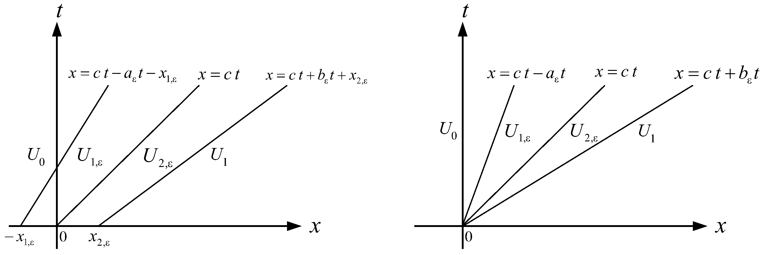
Figure 3.
Interaction of two simple SDW gives the constant SDW (7); , , , , , , , , .
Figure 3.
Interaction of two simple SDW gives the constant SDW (7); , , , , , , , , .

Figure 4.
Approximation of rarefaction waves interactions (intermediate states of are approximated).
Figure 4.
Approximation of rarefaction waves interactions (intermediate states of are approximated).

Figure 5.
Approximation of rarefaction waves interactions (intermediate states of are approximated).
Figure 5.
Approximation of rarefaction waves interactions (intermediate states of are approximated).

Figure 6.
Rarefaction waves that have left after applying described algorithm.

Figure 7.
Phase plane, , .

Figure 8.
Intersection points for , , , .


Table 1.
The intermediate states after solving the problem (1,18) for different , , and . The initial data are , , and , with , ; is the speed of the first left shock , and is the speed of the last right shock ; and are the left-hand sides of the integral form of the first and second equation in (1), respectively; . There are no interactions after .
| 0.1 | 1.90065 | 0.78587 | 0.54812 | 1.03467 | 0.00014 | 0.00029 | 51539.2 |
| 0.05 | 2.42960 | 0.78960 | 0.64243 | 0.94334 | 0.00046 | 0.00091 | 44283.9 |
| 0.01 | 5.97852 | 0.79403 | 0.75266 | 0.83719 | 0.00197 | 0.01341 | 1280.45 |
| 0.009 | 6.45010 | 0.79419 | 0.75643 | 0.83359 | 0.00235 | 0.01775 | 1047.91 |
| 0.007 | 7.78950 | 0.79453 | 0.76426 | 0.82610 | 0.00152 | 0.02834 | 663.973 |
| 0.005 | 10.1816 | 0.79492 | 0.77259 | 0.81822 | 0.00037 | 0.04625 | 379.533 |
| 0.003 | 15.6887 | 0.79570 | 0.78179 | 0.81020 | 0.05231 | 0.05667 | 182.345 |
Table 2.
The intermediate states after solving the problem (1,18) for and . The initial data are , , and , with , ; is the speed of the first left shock , is the speed of the last right shock ; and are the left-hand sides of the integral form of the first and second equation in (1), respectively; . There are no interactions after .
| 6 | 6.45010 | 0.79419 | 0.75643 | 0.83359 | 0.00235 | 0.01775 | 1047.91 |
| 7 | 6.45068 | 0.79418 | 0.75642 | 0.83357 | 0.00109 | 0.00696 | 2381.43 |
| 8 | 6.45058 | 0.79418 | 0.75642 | 0.83357 | 0.00029 | 0.00251 | 5703.15 |
| 9 | 6.45060 | 0.79418 | 0.75641 | 0.83356 | 0.00005 | 0.00203 | 12960.5 |
| 10 | 6.45059 | 0.79417 | 0.75641 | 0.83356 | 0.00001 | 0.00029 | 31037.1 |
Table 3.
The intermediate states after solving the problem (1,18) for different , , and . The initial data are , , and , with , ; is the speed of the first left shock , is the speed of the last right shock ; and are the left-hand sides of the integral form of the first and second equation in (1), respectively; . There are no interactions after .
| 0.1 | 1.74716 | 0.81567 | 0.56896 | 1.05016 | 0.00016 | 0.00004 | 37815.5 |
| 0.05 | 2.22987 | 0.81158 | 0.65838 | 0.95749 | 0.00042 | 0.00007 | 39901.9 |
| 0.01 | 5.47442 | 0.80668 | 0.76348 | 0.84789 | 0.00792 | 0.00948 | 1179.15 |
| 0.009 | 5.90553 | 0.80652 | 0.76708 | 0.84414 | 0.01313 | 0.01241 | 965.899 |
| 0.007 | 7.15678 | 0.80598 | 0.76987 | 0.83954 | 0.02456 | 0.02547 | 635.784 |
| 0.005 | 9.47854 | 0.80512 | 0.77259 | 0.82874 | 0.00037 | 0.04625 | 379.533 |
| 0.003 | 13.7598 | 0.80475 | 0.78815 | 0.81687 | 0.04255 | 0.04113 | 153.487 |
Table 4.
, , .
| Runtime | ||||||||
|---|---|---|---|---|---|---|---|---|
| 0.1 | 1.68612 | 0.828059 | 0.577459 | 1.097462 | 0.00014 | 0.00020 | 0.9 s | (54,245, 93,937) |
| 0.05 | 2.03792 | 0.834141 | 0.674341 | 1.005426 | 0.00037 | 0.00054 | 1.1 s | (62,255, 61,919) |
| 0.01 | 4.22713 | 0.841636 | 0.792563 | 0.894116 | 0.02266 | 0.00402 | 4.8 s | (5127.9, 5734.4) |
| 0.005 | 6.71266 | 0.843121 | 0.815659 | 0.872483 | 0.00501 | 0.02155 | 4477 s | (1229.6, 1408.6) |
| 0.003 | 9.95854 | 0.844183 | 0.826443 | 0.863428 | 0.01212 | 0.00688 | ≈168 h | (812.54, 1008.5) |
| 0.005 * | 6.71283 | 0.843118 | 0.815657 | 0.872480 | 0.00660 | 0.03910 | 15.3 s | (2598.4, 2977.4) |
| 0.003 * | 9.94664 | 0.843848 | 0.826450 | 0.862552 | 0.09700 | 0.05000 | 15.5 s | (894.2, 1036.1) |
* presented algorithm for approximations of interactions was applied.
Table 5.
, , .
| Runtime | ||||||||
|---|---|---|---|---|---|---|---|---|
| 0.1 | 4.22713 | 0.841636 | 0.792563 | 0.894116 | 0.02266 | 0.00402 | 13 s | (5127.9, 5734.4) |
| 0.05 | 4.22717 | 0.841634 | 0.792562 | 0.894115 | 0.00061 | 0.00786 | 25 s | (5122.8, 5728.6) |
| 0.04 | 4.22717 | 0.841634 | 0.792562 | 0.894115 | 0.00059 | 0.00690 | 39 s | (5123.0, 5728.9) |
| 0.03 | 4.22716 | 0.841634 | 0.792562 | 0.894115 | 0.00160 | 0.00691 | 289 s | (5121.2, 5726.9) |
| 0.02 | 4.22716 | 0.841635 | 0.792562 | 0.894115 | 0.00266 | 0.00641 | 1890 s | (5120.4, 5726.0) |
| 0.01 | 4.22716 | 0.841635 | 0.792562 | 0.894115 | 0.00352 | 0.00638 | ≈96 h | (5119.2, 5724.5) |
| 0.02 * | 4.22717 | 0.841634 | 0.792562 | 0.894115 | 0.00819 | 0.00969 | 5.5 s | (14,096, 15,765) |
| 0.01 * | 4.22717 | 0.841634 | 0.792562 | 0.894115 | 0.00690 | 0.01020 | 4.8 s | (14,104, 15,773) |
| 0.005 * | 4.22717 | 0.841634 | 0.792562 | 0.894115 | 0.00600 | 0.009801 | 4.83 s | (14,116, 15,787) |
| 0.001 * | 4.22717 | 0.841634 | 0.792562 | 0.894115 | 0.004487 | 0.014761 | 10.9 s | (14,260, 15,948) |
| 0.0001 * | 4.22717 | 0.841634 | 0.792562 | 0.894115 | 0.01231 | 0.02341 | 62.1 s | (14,347, 16,845) |
* presented algorithm for approximations of interactions was applied.
Disclaimer/Publisher’s Note: The statements, opinions and data contained in all publications are solely those of the individual author(s) and contributor(s) and not of MDPI and/or the editor(s). MDPI and/or the editor(s) disclaim responsibility for any injury to people or property resulting from any ideas, methods, instructions or products referred to in the content. |
© 2024 by the author. Licensee MDPI, Basel, Switzerland. This article is an open access article distributed under the terms and conditions of the Creative Commons Attribution (CC BY) license (https://creativecommons.org/licenses/by/4.0/).
Share and Cite
MDPI and ACS Style
Dedović, N. Approximation of the Interactions of Rarefaction Waves by the Wave Front Tracking Method. Mathematics 2024, 12, 2099. https://doi.org/10.3390/math12132099
AMA Style
Dedović N. Approximation of the Interactions of Rarefaction Waves by the Wave Front Tracking Method. Mathematics. 2024; 12(13):2099. https://doi.org/10.3390/math12132099
Chicago/Turabian StyleDedović, Nebojša. 2024. "Approximation of the Interactions of Rarefaction Waves by the Wave Front Tracking Method" Mathematics 12, no. 13: 2099. https://doi.org/10.3390/math12132099
Note that from the first issue of 2016, this journal uses article numbers instead of page numbers. See further details here.