A Photovoltaic Prediction Model with Integrated Attention Mechanism

Abstract

Solar energy has become a promising renewable energy source, offering significant opportunities for photovoltaic (PV) systems. Accurate and reliable PV generation forecasts are crucial for efficient grid integration and optimized system planning. However, the complexity of environmental factors, including seasonal and daily patterns, as well as social behaviors and user habits, presents significant challenges. Traditional prediction models often struggle with capturing the complex nonlinear dynamics in multivariate time series, leading to low prediction accuracy. To address this issue, this paper proposes a new PV power prediction method that considers factors such as light, air pressure, wind direction, and social behavior, assigning different weights to them to accurately extract nonlinear feature relationships. The framework integrates long short-term memory (LSTM) and gated recurrent units (GRU) to capture local time features, while bidirectional LSTM (BiLSTM) and an attention mechanism extract global spatiotemporal relationships, effectively capturing key features related to historical output. This improves the accuracy of multi-step predictions. To verify the feasibility of the method for multivariate time series, we conducted experiments using PV power prediction as a scenario and compared the results with LSTM, CNN, BiLSTM, CNN-LSTM and GRU models. The experimental results show that the proposed method outperforms these models, with a mean absolute error (MAE) of 12.133, root mean square error (RMSE) of 14.234, mean absolute percentage error (MAPE) of 2.1%, and a coefficient of determination (R²) of 0.895. These results indicate the effectiveness and potential of the method in PV prediction tasks.

1. Introduction

Global warming and climate change have spurred the adoption of renewable energy through legislation and incentives. PV energy is a key sustainable alternative to fossil fuels, crucial for a low-carbon future [1]. PV systems reduce emissions and lessen dependence on fossil fuels, supporting resilient energy systems. PV prediction technology is a crucial tool for optimizing the performance and integration of PV systems into the power grid [2]. The systems generate electricity from sunlight, which makes them highly dependent on the weather conditions. The inherent characteristics of solar energy, including the fluctuation of solar radiation and weather conditions, pose challenges to the reliable and efficient integration of PV energy into power systems. Uncertainties in PV power output can lead to imbalances in supply and demand, potentially impacting grid stability and management. To address these challenges, researchers have focused on developing accurate PV forecasting techniques. Successful PV power forecasting enables grid managers to anticipate fluctuations in power generation, plan resource allocation effectively, and mitigate the effects of intermittent renewable energy sources on the grid.

PV prediction technology is designed to forecast the power output of PV systems by considering a range of factors, including solar radiation, ambient temperature, humidity, and wind speed. The field encompasses a variety of approaches, such as statistical modeling, machine learning algorithms, and numerical weather prediction models. These approaches aim to analyze historical data, meteorological parameters, and PV system characteristics to formulate robust forecasting models. PV predictions can be categorized into two primary methods: indirect and direct [3,4,5,6]. Indirect methods [7,8] utilize predefined mathematical models to predict environmental parameters that influence PV power generation, such as solar radiation [9] and ambient temperature. Techniques for predicting environmental parameters include numerical weather prediction models, statistical models, machine-learning-based approaches, and artificial neural network (ANN) models [10]. Liu and Sun [11] obtained hourly point features similar to the predicted time points through principal component analysis and K-means clustering then used a popular optimization algorithm to quickly select random forest parameters to model the accuracy and robustness of PV power generation prediction. Agoua et al. [12] proposed a statistical approach to address the static nature of PV production data, predicting the situation of PV plants over very short periods. Pan et al. [13] proposed an improved ant colony optimization (ACO) algorithm, which uses the global optimization function of ACO to optimize the parameters of the support vector machine (SVM) model, effectively predicting short-term PV power generation. Jung et al. [14] and Son and Jung [15] predicted PV power generation in the medium and long term based on a LSTM. With the continuous development of neural networks, GRU neural network [16] and BiLSTM neural network [17,18] are also gradually applied to PV power generation prediction.

In addition, by integrating predicted parameters with established PV power generation models, such as equivalent diode models [19], Sandia models [20], and simple efficiency models [21], the power output of PV systems can be inferred. These indirect methods offer valuable insights into the expected performance of PV systems, providing essential tools for estimating system performance based on environmental conditions.

On the other hand, direct PV prediction methods [22,23,24] foretell the power output of PV systems by directly analyzing historical data and relevant meteorological variables. These methods typically employ techniques like support vector regression (SVR), neural networks, and hybrid neural network models. SVR [25] is adept at uncovering nonlinear relationships and complex feature interactions to predict PV power output. Neural networks, including deep learning architectures [26,27,28], learn patterns from historical PV power output and meteorological data to make accurate predictions. Hybrid models, which may incorporate LSTM, GRU, and CNN, improve prediction accuracy by capturing both short-term and long-term dependencies. For example, Wang et al. [29] developed a prediction model based on long short-term memory recurrent neural network (LSTM-RNN), incorporating the principle of temporal correlation to accurately predict day-ahead PV power. Lim et al. [30] proposed a hybrid model consisting of CNN and LSTM, where CNN classifies weather conditions and LSTM learns power generation patterns based on these conditions for stable power generation prediction. Chen et al. [31] proposed four different deep-learning-based hybrid models to predict short-term PV power generation, using Bayesian optimization (BO)-based LSTM and CNN, respectively, considering the effects of stochastic and intermittent solar radiation on PV prediction. Other relevant references can be found in [32,33,34].

Generally, most direct methods surpass the indirect methods in the general task of forecasting future PV power output [35]. Although these methods demonstrate effective PV power prediction, SVR methods [36,37] usually incur substantial computational time, which limits their applicability to large datasets. Additionally, existing studies reveal a limitation in the learning models of ANN-based approaches. Given the intricate nature of weather systems, such models may inadequately extract the nonlinear and static features present in PV power data. Thus, optimizing ANNs to enhance accuracy becomes crucial for achieving better performance. Jawaid et al. [38] provide a comparative analysis of different ANN algorithms, albeit without disclosing specific details of their prediction models or numerical performance. For instance, single algorithms, such as SVM, are ill-suited for large-scale data and necessitate precise parameter tuning. Random forest algorithms are susceptible to overfitting and lengthy training times, while LSTM-based algorithms are prone to gradient vanishing and explosion issues.

Attentional mechanisms, complex resource allocation strategies in neural networks that effectively direct computational resources to prioritize critical tasks, have been shown to have significant potential for improving the performance of various neural network architectures and have been progressively applied to sequence prediction problems. Cinar et al. [39] developed an extended attention model for recurrent neural networks (RNNs). Experiments show that the model can effectively capture pseudo-periodicity in time series and significantly outperforms traditional RNN models. Wang et al. [40] proposed a hybrid model combining quadratic decomposition (SD), multifactor analysis (MFA), and attention-based long short-term memory network (ALSTM) for predicting the country’s stock market price trends. The empirical analysis shows that the proposed model improves at least 30% in accuracy compared to the standard LSTM, which validates the hybrid model effectiveness.

Considering the limitations of traditional artificial intelligence methods, such as overfitting and limited generalization in complex nonlinear modeling, this paper proposes a hybrid model to address these issues. Accurate and stable PV prediction, particularly for long time series, is crucial. Traditional statistical methods, while effective at modeling logical correlations in data, often struggle to capture the connections in serial data patterns. In contrast, neural network approaches have gained attention for their superior ability to handle forecasting challenges. However, different network structures exhibit varying sensitivities and capabilities in managing PV series data. To leverage the strengths of various network structures, this paper proposes a hybrid approach that integrates multiple structural modules within a neural network architecture. This hybrid model aims to enhance reliability and accuracy in PV prediction. The main contributions and implications of this paper are listed as follows:

(1) We propose a hybrid neural network framework for PV prediction that combines the structural modules of LSTM, GRU, and BiLSTM integrated with an attention mechanism. This framework is designed to achieve multi-step future PV data forecasting using multiple feature inputs. By incorporating the influential weights of factors such as light, wind direction, air pressure, and behavior patterns, the model enhances the accuracy of PV predictions.

(2) The proposed model in this study highlights the importance of fusing multiple input features to effectively capture key factors related to historical output and fully extract the inherent nonlinear and static features in PV data to further improve prediction performance. By introducing a hybrid model architecture of GRU, LSTM, and BiLSTM, the advantages of each model are leveraged to handle different time series features. The attention mechanism is combined to dynamically focus on important time steps, significantly improving the prediction accuracy and stability of the model.

(3) We conducted extensive experiments on a PV dataset collected in Wuhan, China, to evaluate the effectiveness of the proposed model for PV prediction. The empirical results demonstrate significant improvements over baseline methods, highlighting the model’s enhanced accuracy and robustness.

The rest of the paper is organized as follows: Section 2 describes the model structures of the neural networks used. Section 3 details the data and evaluation indicators employed in the experiments and presents and explains the numerical analysis results. Finally, Section 4 concludes the paper with a summary of the findings.

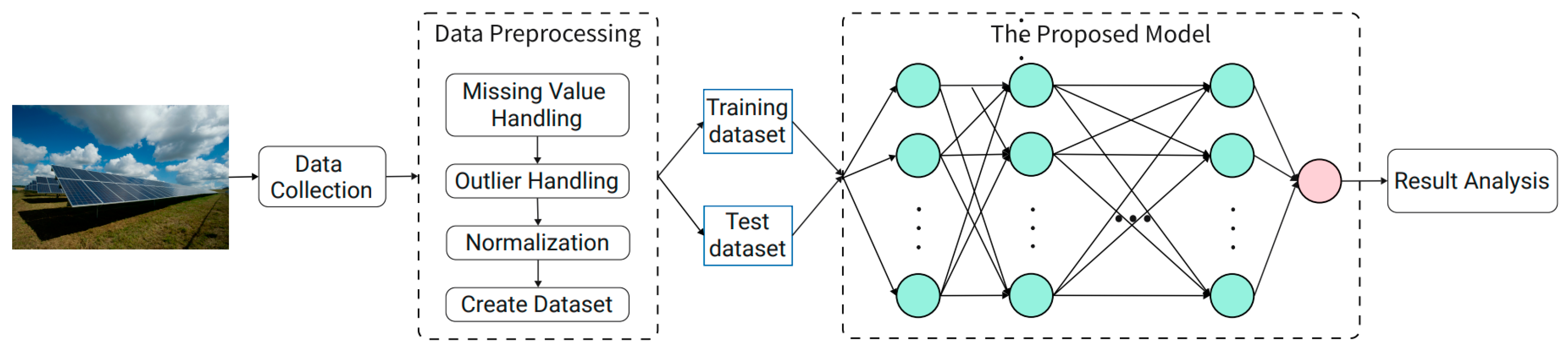
2. Materials and Methods Proposed Photovoltaic Prediction Model

2.1. Description of the Prediction Problem

The various influencing factors of n-step historical data and the corresponding PV power are taken as a multivariate input, and the input data are defined as X = [${\mathbf{x}}_{\mathbf{1}}$, ${\mathbf{x}}_{\mathbf{2}}$, …, ${\mathbf{x}}_{\mathbf{m}}$], where ${\mathbf{x}}_{\mathbf{i}}$ = [${\mathbf{x}}_{\mathbf{i}(\mathbf{t}-\mathbf{n}+\mathbf{1})}$, ${\mathbf{x}}_{\mathbf{i}(\mathbf{t}-\mathbf{n}+\mathbf{2})}$, …, ${\mathbf{x}}_{\mathbf{i}\left(\mathbf{t}\right)}$] represents a multivariate input, ${\mathbf{x}}_{\mathbf{i}\left(\mathbf{j}\right)}$ = [${\mathrm{x}}_{1\mathrm{j}}$, ${\mathrm{x}}_{2\mathrm{j}}$, …, ${\mathrm{x}}_{\mathrm{q}\mathrm{j}}$] represents the jth time step in the multivariate input ${\mathbf{x}}_{\mathbf{i}}$, and ${\mathrm{x}}_{\mathrm{p}\mathrm{j}}$ represents the pth element in the time step, where the first q − 1 elements are the various influencing factors affecting the PV power, and the qth element is the PV power at the time step. The true value set of the PV power predicted for the next time step is defined as Y = [${\mathrm{y}}_1$, ${\mathrm{y}}_2$, …, ${\mathrm{y}}_{\mathrm{m}}$], a subset of X and Y trainX and trainY are separated for training, and the remaining sets testX and testY are used for verification. The goal of this paper is to find a function model f; for any given input X, the predicted value $\widehat{\mathbf{Y}}$ = f (X) output by the model can be as close to the true value Y as possible.

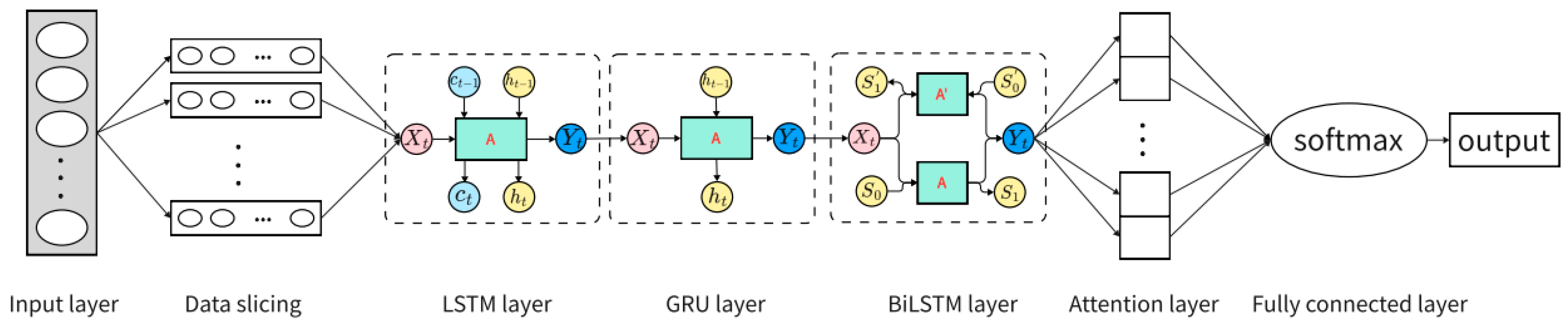
2.2. The Structure of the Network

The workflow of the proposed model is shown in Figure 1 and follows a structured process. First, the power data and various influencing factors of the photovoltaic device are collected to obtain the raw data to be processed. In the process of dataset creation, missing value processing, outlier processing, and normalization operations are performed, and the data within a fixed time step are used as a multivariate input using a sliding window method. Subsequently, the created dataset is divided into a training set and a test set according to a predetermined ratio. The training data are then input into the network to be trained, and a certain number of iterations are performed to obtain the trained model; then, the test data are input to obtain the test output results, and finally, the results are analyzed.

2.2.1. Long Short-Term Memory Networks (LSTM)

For the input signal $X_t$ at a given current moment, and the state $h_{t-1}$ of the hidden layer at the previous moment, the value of the memory gate $i_t$, the forgotten door $f_t$, and the temporary cell state ${\tilde{C}}_t$ can be calculated with the following Formulas (1)–(3):

$$i_t=\sigma (W_i·{[h}_{t-1},x_t]+b_i),$$

(1)

$$f_t=\sigma (W_f·[h_{t-1},x_t]+b_f),$$

(2)

$${\tilde{C}}_t=tanh(W_C·[h_{t-1},\mathrm{}{x}_t]+b_C).$$

(3)

For the calculated value of the memory gate $i_t$, the forgotten door $f_t$, and the temporary cell state ${\tilde{C}}_t$, the state of the cell at the previous moment $C_{t-1}$ and the state of the cell at the current moment $C_t$ can be calculated according to the listed Formula (4):

$$C_t=f_t\ast C_{t-1}+i_t\ast {\tilde{C}}_t.$$

(4)

For the given previous moment of the state $h_{t-1}$, the input signal $X_t$, and the calculated cell state at the current moment $C_t$, the state of the hidden layer $h_t$ at the current moment can be calculated using the following Formula (5); the hidden cell structure of the LSTM is shown in Figure 2.

$$h_t=\sigma (W_o·[h_{t-1},\mathrm{}{x}_t]+b_o)\ast tanh\left(C_t\right)$$

(5)

2.2.2. Gated Recurrent Unit Neural Network (GRU)

For a given state $h_{t-1}$ at the previous moment and input $X_t$ of the current node, the state of the two gates can be calculated according to Formulas (6) and (7), where $r_t$ is the state of the reset gate and $z_t$ is the current state of the update gate:

$$z_t=\sigma (W_z·[h_{t-1},x_t]+b_z),$$

(6)

$$r_t=\sigma (W_r·[h_{t-1},x_t]+b_r).$$

(7)

For the obtained gate signal, we first use the reset gate to obtain the reset data then splice it with the input signal $X_t$ and finally convert the data to the range (−1, 1) through the activation function $tanh$ to obtain the ${\tilde{h}}_t$; Formula (8) is provided as follows:

$${\tilde{h}}_t=tanh(W·[r_t\ast h_{t-1},x_t]+b).$$

(8)

Finally, the module is updated using the update gate, as shown in the following Formula (9):

$$h_t=\left(1-z_t\right)\ast h_{t-1}+z_t\ast {\tilde{h}}_t.$$

(9)

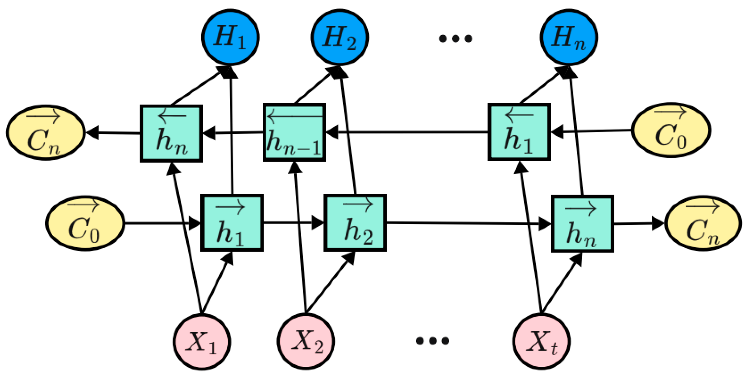
2.2.3. Bidirectional Long Short-Term Memory (BiLSTM) Neural Network

The BiLSTM [41] neural network structure model is divided into two independent LSTMs, and the input sequence is input into the two LSTM neural networks in positive and reverse order for feature extraction, and the word vector formed after the splicing of the two output vectors (that is, the extracted feature vector) is used as the final feature expression of the word so that the feature data obtained at moment t have both past and future information. Figure 3 shows the overall implementation process of BiLSTM.

As can be seen from Figure 3, BiLSTM takes LSTM as the hidden element, the input features enter the model structure in two different directions, and the output vectors of the two hidden elements at the moment are connected to form the output at that moment, where ${\mathrm{H}}_1$, ${\mathrm{H}}_2$… ${\mathrm{H}}_{\mathrm{n}}$ represents the output vector. Let the input at time t be ${\mathrm{H}}_{\mathrm{t}}$, the output state of the forward LSTM layer be ${\overrightarrow{\mathrm{h}}}_{\mathrm{t}}$, the output state of the reverse LSTM layer be ${\overleftarrow{\mathrm{h}}}_{\mathrm{t}}$, and the output vector at this time be ${\mathrm{H}}_{\mathrm{t}}$; then, the calculation of BiLSTM at time t is shown in Equations (10)~(12).

$${\overrightarrow{h}}_t=LSTM(x_t,{\overrightarrow{h}}_{t-1})$$

(10)

$${\overleftarrow{h}}_t=LSTM(x_t,{\overleftarrow{h}}_{t-1})$$

(11)

$$H_t=\overrightarrow{W}{\overrightarrow{h}}_t+\overleftarrow{W}{\overleftarrow{h}}_t+b_H$$

(12)

2.2.4. Attention Mechanism

In view of the fact that there may be ignorance of the effective use of key feature information in the model, the learning of time series feature information via mechanism attention is increased. The mechanism calculates the feature weight ${\alpha }_t$ by outputting vector $h_t$ as input at the upper time t, and the calculation is shown in Equations (13)~(15):

$$u_t=\mathrm{}\mathrm{t}\mathrm{a}\mathrm{n}\mathrm{h}\left(W_a{h}_t+b\right),$$

(13)

where $W_a$ is the weight coefficient; $b$ is the bias coefficient;

$${\alpha }_t=\frac{\mathrm{e}\mathrm{x}\mathrm{p}\left(u_t^{\mathrm{T}}{u}_{\omega }\right)}{\sum _t\mathrm{e}\mathrm{x}\mathrm{p}(u_t^{\mathrm{T}}{u}_{\omega })},$$

(14)

where a is the initialization weight matrix;

$$C_t={\sum }_t{\alpha }_t{h}_t.$$

(15)

By calculating the importance of the output at time t to the result $u_t$, the feature weight ${\alpha }_t$ of $h_t$ is calculated, the vector $C_t$ is output, and the input index vector at time t is weighted. The larger the calculated weight ${\alpha }_t$, the greater the importance of the hidden layer features at that moment, and the greater the contribution of vector $C_t$ to the prediction results at that moment. Through the above calculations, the model is finally output ${y\prime }_i$ via the softmax activation function in the fully connected layer, as shown in Equation (16).

$${y\prime }_i=softmax(W_i{C}_t+b_i)$$

(16)

2.3. The Prediction Model Composition

Figure 4 depicts the structure of our proposed model, which involves several interconnected layers. The input format of the model is initially determined by a defined lookback. The LSTM layer with LeakyReLU activation consists of 100 neurons, whose output are connected to a GRU layer with ReLU, which contains 100 neurons. The initial layers, comprising LSTM and GRU units, possess strong memory and long-range dependency capture capabilities, effectively addressing the limitations of traditional RNNs. The data then pass through a bidirectional LSTM layer, composed of LSTMs with 128 neurons and the ReLU activation function, enabling effective information capture from both past and future contexts, thereby enhancing sequence understanding and prediction. The subsequent layers include batch normalization to stabilize the input data distribution and accelerate model learning, dropout layers to prevent overfitting, and the integration of an attention mechanism to facilitate enhanced learning and assign weights between different data points. For attention mechanism functions, when encountering anomalous transitions between different time series features, the weights can be adaptively adjusted in real time to help extract time series data associations. In this way, when the prediction is validated, the predicted output of the anomaly relationship can be better transformed. Following these layers, another batch normalization layer and dropout layer are implemented. Finally, the data are flattened and input into a linear dense layer with softmax activation function for output. Through this comprehensive network structure, our proposed model achieves enhanced sequence prediction capabilities by combining various advanced techniques and leveraging the strengths of each layer.

2.4. Training Strategy of the Proposed Model

The training process of the proposed model begins by preparing the dataset, which consists of historical PV power output and corresponding meteorological data. Algorithm 1 provides the strategy of our dataset creation. The dataset is divided into training and validation sets to evaluate the model’s performance during training.

Algorithm 1: The strategy of our dataset creation.

Input: the raw data table dataset, the predicted step size of the slide look_back.

Output: Training Sample $X_{train}$, Training Label $Y_{train}$, Test Sample $X_{test}$, Test Label $Y_{test}$.

1: Data preprocessing (dataset)

2: DataInitialize (X, Y)

3: For i in len (dataset)

4:  X, Y ← CreateData (dataset, look_back)

5: End For

6: ($X_{train}$, $X_{test}$), ($Y_{train}$, $Y_{test}$) ← (α*X, (1 − α)*X), (α*Y, (1 − α)*Y)

7: End

The network is trained using an iterative process that involves feeding batches of input data into the model, calculating the predicted PV power output, and comparing it with the actual output. The difference between the predicted and actual values is measured using the appropriate loss function of mean squared error (MSE).

During training, the model learns to optimize its internal parameters through a gradient-based optimization algorithm stochastic gradient descent (SGD). The gradients are computed using backpropagation, allowing for adjustments to the weights and biases of the network in order to minimize the loss function and improve prediction accuracy. To prevent overfitting, regularization techniques like dropout or L1/L2 regularization may be applied, which encourage the network to learn more robust and generalizable patterns from the data.

The training process involves iterating through multiple epochs, where each epoch represents a complete pass through the entire training dataset. After each epoch, the model’s performance on the validation set is evaluated to monitor its generalization ability and prevent overfitting. The validation metrics of root mean squared error (RMSE) and R-squared (${\mathrm{R}}^2$) value provide insights into the model’s predictive performance. The training continues until the model achieves satisfactory performance on the validation set or reaches a predefined stopping criterion, such as a maximum number of epochs or no significant improvement in validation metrics. The training strategy of the proposed model for PV prediction is demonstrated in Algorithm 2. Upon completing the whole training process, the proposed model is capable of generating accurate predictions of PV power output based on the input meteorological data, which fully enables reliable forecasts for future PV energy generation.

Algorithm 2: Training strategy of the proposed model for PV Prediction.

Input: number of training iterations epoch, batch size of the dataset B, learning rate $L_{learning\_rate}$, training set $X_{train}/Y_{train}$, test set $X_{test}/Y_{test}$

Output: model training loss function $L_{loss}$, parameters of the network model trained for the i th time ${\theta }_i$.

1: Initialize ${\theta }^0$

2: For i in epoch

3:  $X_{train}^B$, $Y_{train}^B$ ← GetMiniBatch ($X_{train}$, $Y_{train}$, B)

4:  ${\mathrm{V}}_1$ ← LSTM ($X_{train}^B$)

5:  $V_2$ ← GRU ($V_1$)

6:  $V_3$ ← BiLSTM ($V_2$)

7:  $V_4$ ← Dropout ($V_3$)

8:  A ← Attention ($V_4$)

9:  $L_{logits}$ ← Matmul ($A,{\theta }_i$)

10:  O ← Dense (Flatten (A))

11:  $L_{loss}$ ← mean_squared_error ($O,Y_{train}^B$)

12:  ${\theta }_i$ ← Adam ($L_{learning\_rate}$, $L_{loss}$)

13: End For

14: Evaluate ($X_{test}$$,Y_{test}$$,\theta$)

15: End

3. Experimental Evaluations

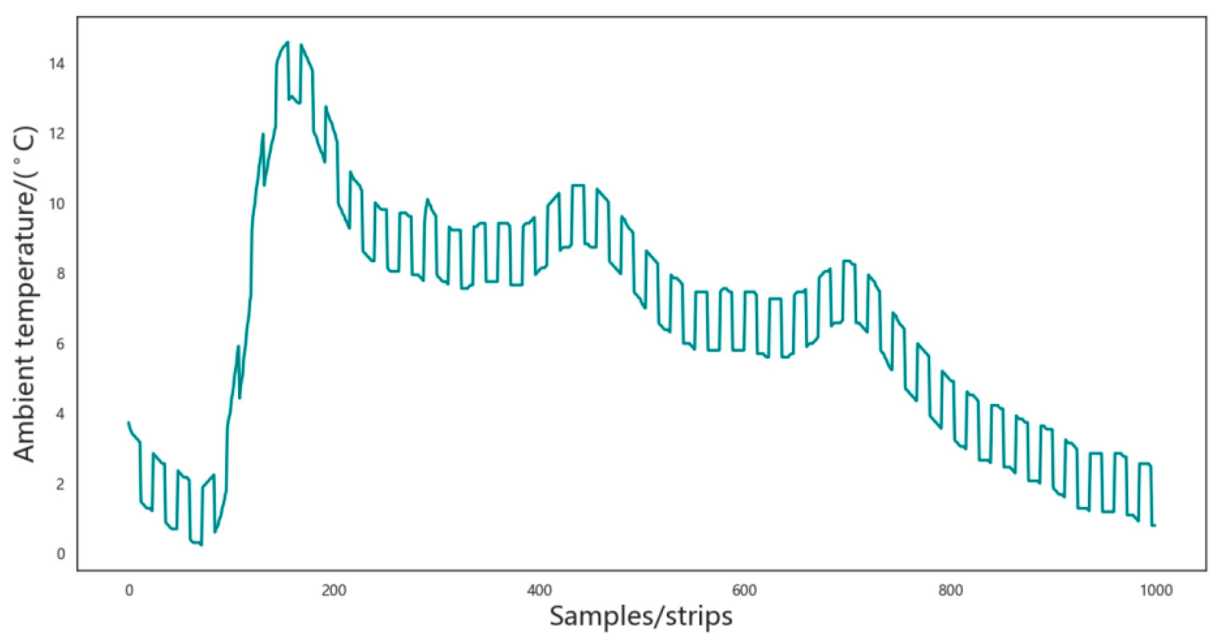
3.1. Data Description

The dataset is a power station situated in Wuhan, Hubei Province, China, involving weather and historical PV actual generation power data with 5 min resolution from January 2021 to December 2023; one data point every five minutes of a day, 288 data points a day, which amounts to a total of 310,000 datasets. This station serves as a pivotal hub for collecting comprehensive solar energy performance metrics, which offers valuable insights into the dynamics of solar power generation in the region. The dataset encompasses PV power values and a range of weather indicators that are crucial for understanding and predicting the efficiency and output of solar panels. The dataset encompasses PV power values and a range of weather indicators that are crucial for understanding and predicting the efficiency and output of solar panels. These key weather parameters typically include global horizontal irradiance (GHI), direct normal irradiance (DNI), diffuse horizontal irradiance (DHI), ambient temperature, relative humidity, wind speed and direction, and precipitation, totaling seven attributes. Capturing seasonal variations and unusual weather events requires the collection of high-frequency data (e.g., hourly or even more frequently), which is typical practice to accurately reflect real-time fluctuations in solar irradiance and weather conditions. These data are essential for the precise modeling and forecasting of PV system performance.

3.2. Data Pre-Processing

In the process of dataset creation, missing value processing, outlier processing, and normalization operations are performed, and the data within a fixed time step are used as a multivariate input using a sliding window method. The feature data in this study exhibit significant scale differences. To mitigate the impact of these discrepancies, the dataset was normalized. This normalization process helps accelerate the convergence of the loss function, prevents gradient explosion during network training, and enhances computational accuracy. The min–max normalization method was employed to scale the data to the [0, 1] range, as illustrated in Equation (17):

$${x\prime }_i=\frac{x_i-x_{min}}{x_{max}-x_{min}},$$

(17)

where $x_i$ is the raw data, ${x\prime }_i$ is the normalized value, and $x_{min}$ and $x_{max}$ are the minimum and maximum values of the original data, respectively. Since the data normalized by the model are also normalized, the output data are denormalized through a flipping process. The calculation formula is shown in Equation (18).

$$\widehat{x}=y^{\prime }\left(x_{max}-x_{min}\right)+x_{min},$$

(18)

where $y\prime$ is the normalized PV prediction. ($\widehat{x}$ is the actual PV prediction obtained after reverse normalization.) Figure 5 and Figure 6, given below, show the results before and after normalization of the ambient temperature indicator.

3.3. Evaluation Indicators

To compare the performance of the proposed model against a single neural network, the experiment incorporates the following regression evaluation indicators [42] (where ${\mathrm{y}}_{\mathrm{i}}$ represents the true value and ${\widehat{\mathrm{y}}}_{\mathrm{i}}$ represents the predicted value) to quantify the overall prediction error.

Mean absolute error (MAE): The indicator MAE measures the average absolute difference between the predicted and true values. A smaller MAE indicates a better accuracy of the predictive model. The value range of the indicator is [0, +∞], where

$$MAE=\frac{1}{n}{\sum }_{i=1}^n|{\widehat{y}}_i-y_i|.$$

(19)

Root mean square error (RMSE): This indicator calculates the square root of the average squared deviation between the predicted and true values. A smaller RMSE indicates better accuracy. The value range of RMSE is [0, +∞]. The calculation of the indicator is shown in the following formula:

$$RMSE=\sqrt{\frac{1}{m}{\sum }_{i=1}^m{{(y}_i-{\widehat{y}}_i)}^2}.$$

(20)

Average absolute percentage error (MAPE): This indicator quantifies the average percentage difference between the predicted and true values, considering the true values as a reference. A smaller MAPE indicates higher accuracy. The value range of MAPE is [0, +∞].

$$MAPE=\frac{1}{n}{\sum }_{i=1}^n\left|\frac{{\widehat{y}}_i-y_i}{y_i}\right|$$

(21)

R-squared (${\mathrm{R}}^2$): This indicator assesses the proportion of variation in the dependent variable that can be explained by the independent variables. A higher ${\mathrm{R}}^2$ value indicates a better model fit. The value range of the ${\mathrm{R}}^2$ is [0, 1]. The closer the value is to 1, the better the prediction model fits, whose calculation formula is demonstrated as follows:

$$R^2=1-\frac{{\sum }_i{{(y}_i\mathrm{}-\mathrm{}{\widehat{y}}_i)}^2}{{\sum }_i{{(y}_i\mathrm{}-\mathrm{}{\overline{y}}_i)}^2}.$$

(22)

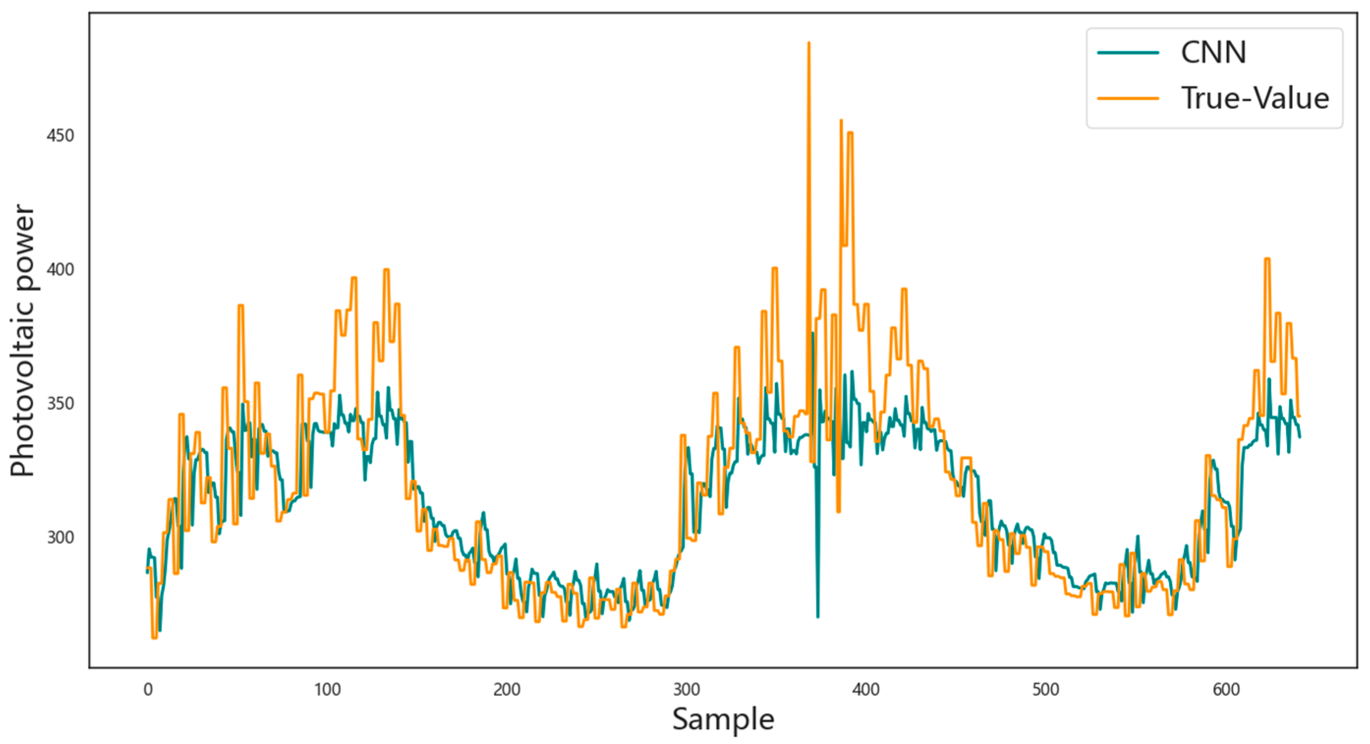
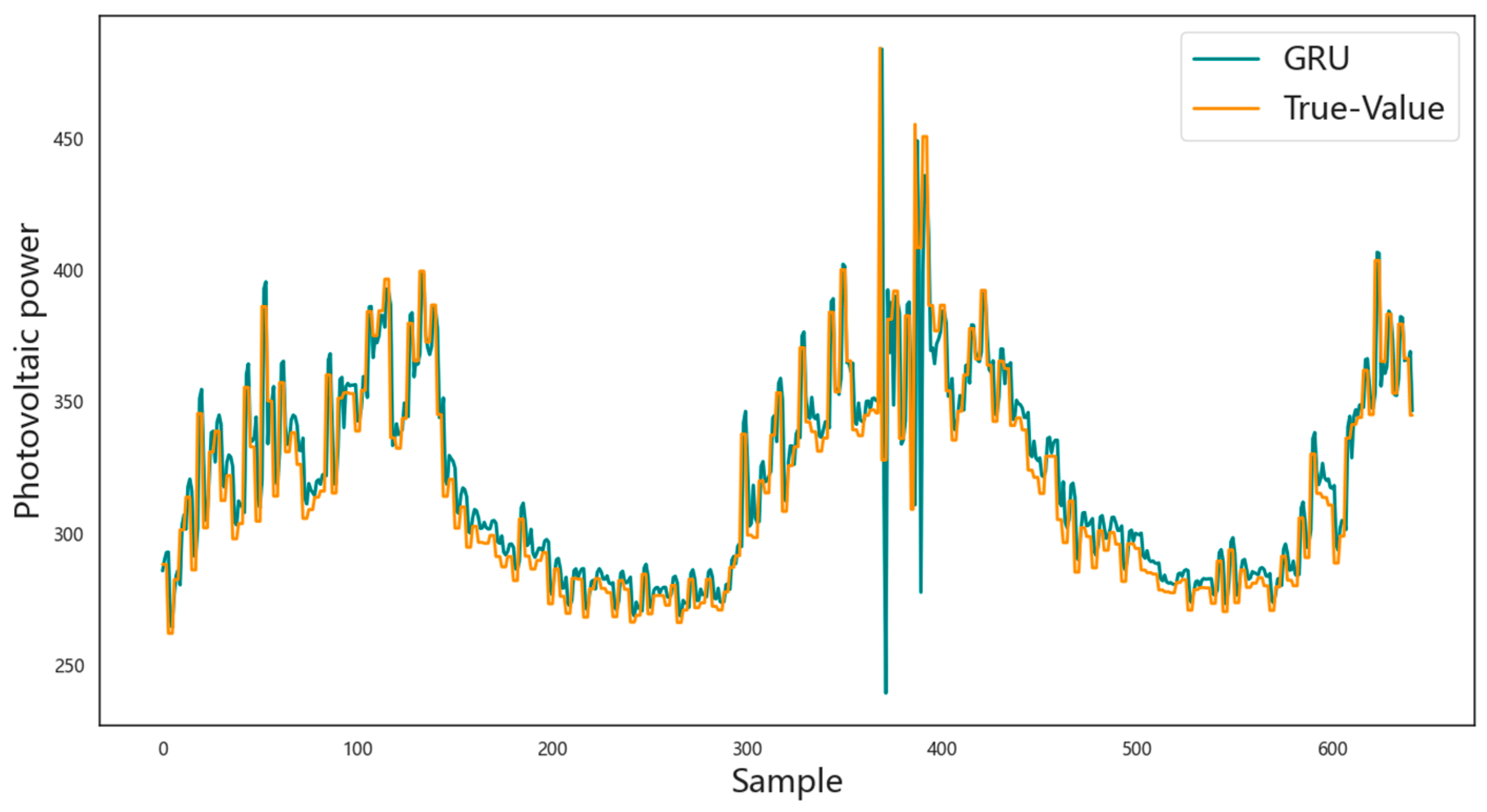
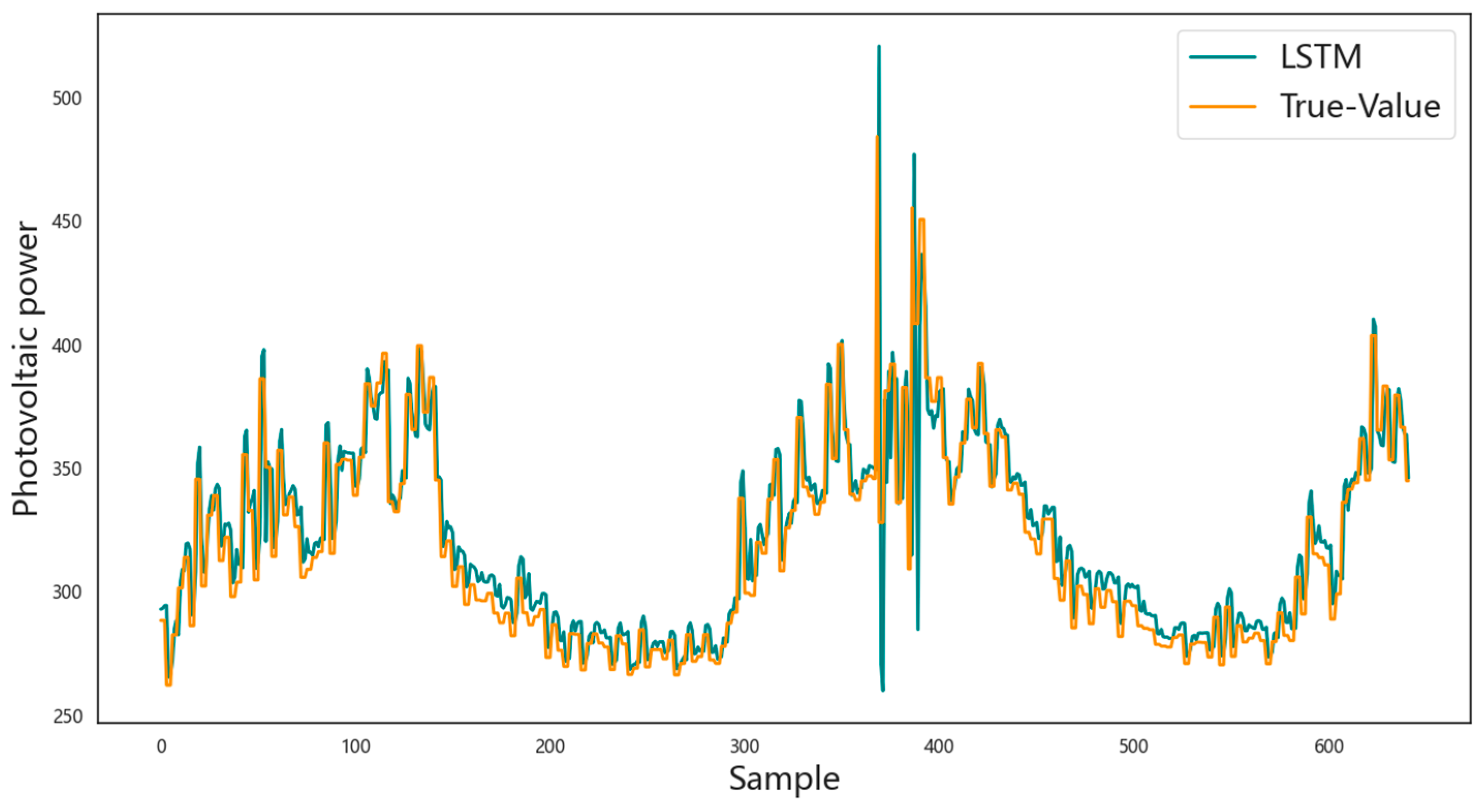
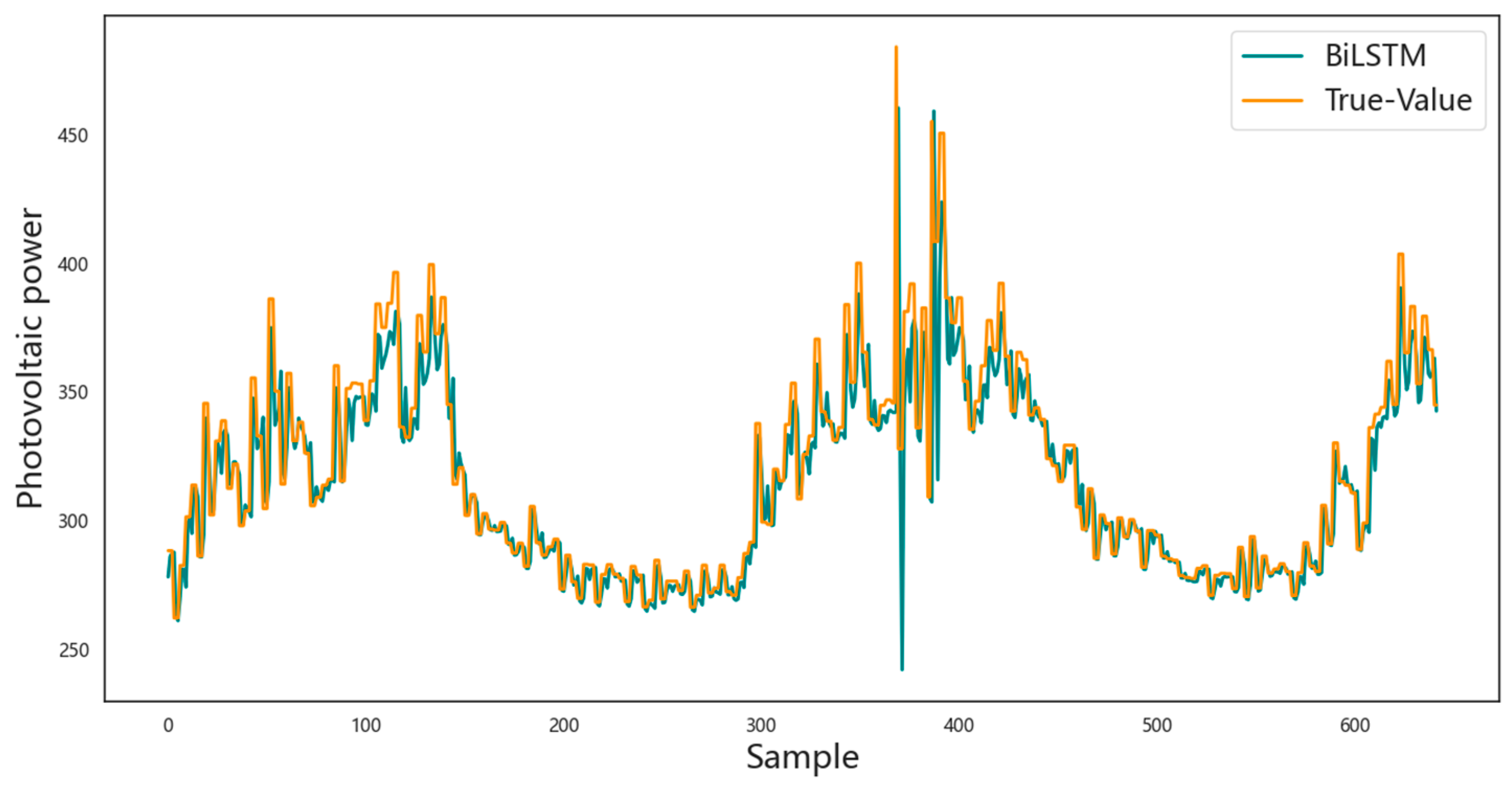
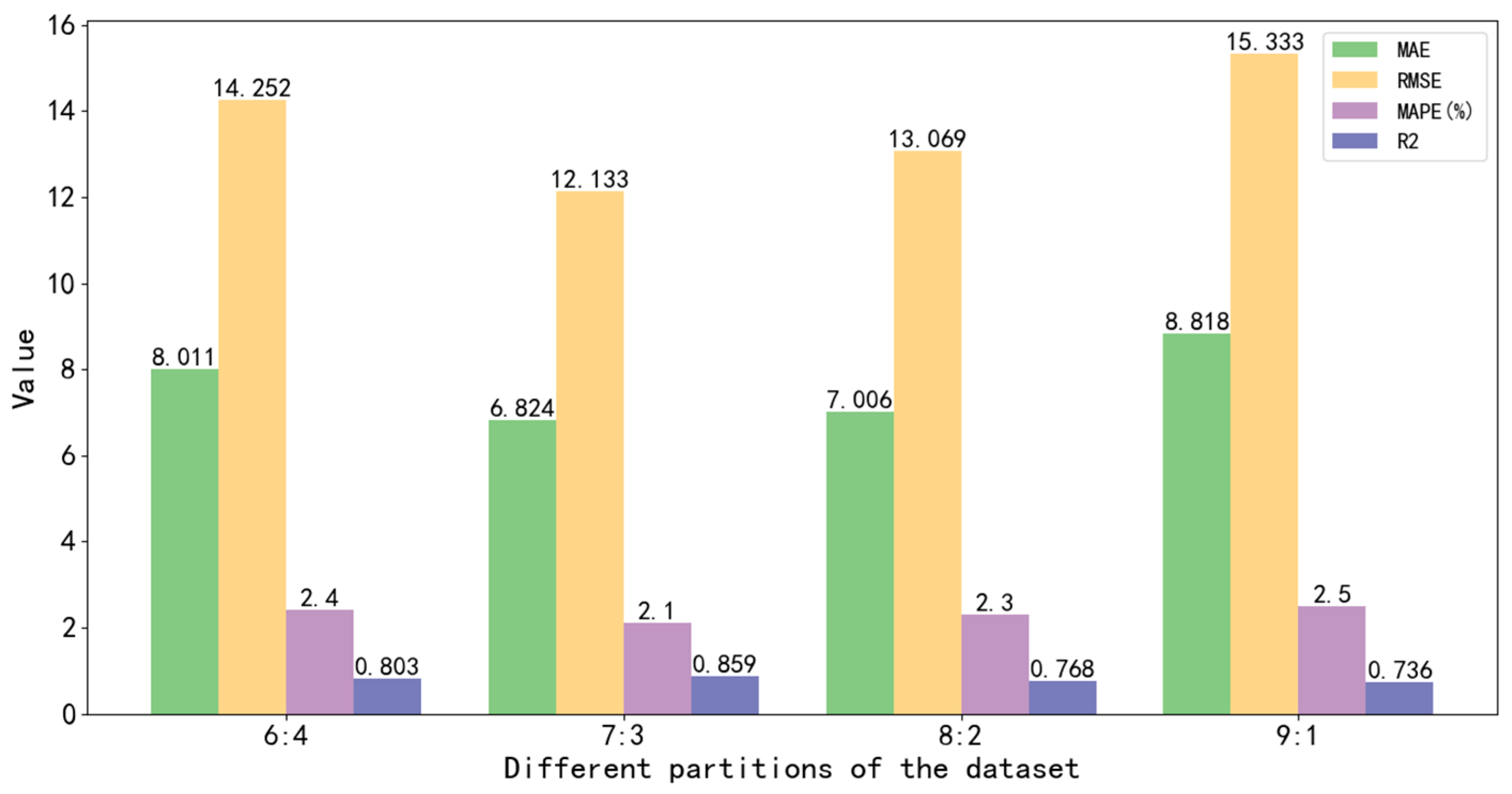
3.4. Prediction Results Analysis

In order to further verify the superiority of the prediction model based on the long short-term memory network proposed in this paper in photovoltaic power prediction, the CNN model, GRU model, LSTM model, BiLSTM model, and CNN-LSTM model are selected as comparative models for analysis. Each comparative method is tested and analyzed based on the entire dataset, of which 70% of the data are used for training, and the remaining 30% of the data are used for prediction. The prediction results are shown in Figure 7, Figure 8, Figure 9, Figure 10, Figure 11 and Figure 12, respectively. The horizontal axis represents the sample, the vertical axis represents the photovoltaic power, the orange solid line is the actual photovoltaic power, and the blue solid line is the photovoltaic power predicted by the corresponding model. In each figure, the closer the two curves are, the better the model effect is. It can be observed that the prediction result curve of the network model proposed in this paper is closest to the curve of the actual data, and compared with the prediction results of the other five models, the prediction accuracy of the photovoltaic power of this model is higher, and the changes in the predicted value and the actual value are more consistent.

The above comparison with a line chart is very intuitive, but it is also a bit rougher. To quantify the comparison of the predicted results, for the four models with this indicator, the values of the four quantities calculated by Equations (19)–(22) are shown in

Table 1. Based on the fact that the ratio of the training set to the test set is 7:3, the PV prediction evaluation indexes obtained by various methods are compared.

Evaluation Indicators	MAE	RMSE	MAPE (%)	${\mathbf{R}}^2$
GRU	7.674	14.123	2.6	0.852
LSTM	7.334	13.978	2.5	0.874
CNN	12.912	25.589	3.3	0.743
BiLSTM	8.193	16.532	2.8	0.820
CNN-LSTM	10.559	19.056	3.0	0.761
The proposed model	6.824	12.133	2.1	0.895

, where the best results in the models are represented in bold.

As can be seen from Table 1, the prediction accuracy is from high to low in the order of the proposed model: LSTM, GRU, BiLSTM, CNN-LSTM, and CNN. In terms of MAE indicators, the proposed model is 0.51, 0.85, 6.088, 1.369, and 3.735 lower than the single LSTM, GRU, CNN, BiLSTM, and CNN-LSTM models, respectively. The RMSE of the proposed model for photovoltaic power prediction is 12.133, which is 1.854, 1.99, 13.456, 4.399, and 6.923 lower than the single LSTM, GRU, CNN, BiLSTM, and CNN-LSTM, respectively. In terms of MAPE, the proposed model is 0.4%, 0.5%, 1.2%, 0.7%, and 0.9% lower than the single LSTM, GRU, CNN, BiLSTM, and CNN-LSTM, respectively, which further quantitatively verifies the rationality and effectiveness of the model proposed in this paper.

From the above experiments, it can be seen that the model proposed in this paper has strong stability and robustness. It can be seen that the single-layer GRU or LSTM network performs better than CNN in predicting long-term time series data. This is mainly because CNN is more suitable for spatial feature extraction and cannot capture the dependencies before and after the sequence. LSTM and GRU networks can effectively capture the dependencies of long sequences, thereby achieving more accurate predictions. However, these single-module networks do not fully consider the spatiotemporal relationship and the weight distribution of influencing factors when making predictions. Therefore, the proposed model adds BiLSTM, which allows for better utilization of past and future features at any given moment, thereby enhancing the prediction of future data, and integrates the attention mechanism to consider the weight distribution of influencing factors. There is still a slight deviation between the predicted data and the real data near consecutive peaks or troughs. This difference can be attributed to the inherent limitations of LSTM and GRU models in processing long sequences and effectively utilizing past and future data features.

In order to further verify the robustness and reliability of the proposed model, the dataset was divided into different ratios, and the ratios of training data to test data were 6:4, 7:3, 8:2, and 9:1. Figure 13 shows the performance indicators of the proposed model on different divided datasets.

It can be clearly seen from Figure 13 that when the training data are small, the model does not converge to the optimal index, but as the proportion of training data increases, the MAE, RMSE, and MAPE indicators of the model gradually increase, and the ${\mathrm{R}}^2$ indicator decreases, indicating that the performance of the model gradually decreases, and the generalization ability of the model decreases, but the overall index is still good. It can be concluded that the proposed model has good robustness in photovoltaic power prediction, and it is very important to choose a suitable ratio of training data to test the data. Therefore, in the previous comparative experiments, a 7:3 division of training data and test data was used.

In terms of evaluation metrics, our method performs well in MAE, RMSE, ${\mathrm{R}}^2$, and MAPE, indicating more accurate prediction, higher robustness, and more stable performance. The inherent advantages of our method are summarized as follows:

(1) Enhanced expressive ability: Different types of neural network layers exhibit unique strengths when processing data, and by combining them, we can integrate their respective expressive capabilities, thereby improving the overall modeling ability of the network. This enables more accurate modeling of complex data relationships.

(2) Overfitting inhibition: In some cases, a single type of neural network layer may be prone to overfitting the training data. However, by introducing different layers, particularly those with strong regularization techniques, the connected structural modules mitigate the risk of overfitting and enhance the model’s generalization ability.

(3) Adaptive feature learning: The proposed model processes data through different types of layers multiple times, allowing the model to adaptively learn various features in the data. This multi-level feature learning enables better capture of the complexity inherent in the data.

(4) Better focus on important information: The attention mechanism enables the network to automatically prioritize the most informative parts of the sequence data. This is especially important for forecasting tasks, as some features in photovoltaic power data can significantly affect the forecast results. By combining the attention mechanism with LSTM or GRU, the network can dynamically enhance or weaken the influence of features at different time steps, thereby improving forecast accuracy.

4. Conclusions

This paper proposes a novel and efficient connection model for general photovoltaic forecasting tasks. It combines LSTM structural modules, gated recurrent units and BiLSTM, and is combined with an attention mechanism to effectively learn bidirectional sequential photovoltaic data and capture key features related to historical outputs, thereby achieving accurate multi-step forecasting. Experimental results show that the proposed model has a mean absolute error (MAE) of 6.824, a root mean square error (RMSE) of 12.133, a mean absolute percentage error (MAPE) of 2.1%, and a determination coefficient of 0.895, all of which are better than other networks, indicating that the proposed model performs well in large-scale photovoltaic data forecasting, showing the effectiveness and great potential of the model in PV tasks. Therefore, this method can provide power grid managers with an intelligent decision-making system for photovoltaic forecasting to ensure effective planning of resource allocation.

References

1. Dubey, S.; Sarvaiya, J.N.; Seshadri, B. Temperature dependent photovoltaic (PV) efficiency and its effect on PV production in the world–a review. Energy Proc. 2013, 33, 311–321. [Google Scholar] [CrossRef]
2. Li, Y.; Song, L.; Zhang, S.; Kraus, L.; Adcox, T.; Willardson, R.; Lu, N. A TCN-based hybrid forecasting framework for hours-ahead utility-scale PV forecasting. IEEE Trans. Smart Grid 2023, 14, 4073–4085. [Google Scholar] [CrossRef]
3. Das, U.K.; Tey, K.S.; Seyedmahmoudian, M.; Mekhilef, S.; Idris, M.Y.I.; Van Deventer, W.; Stojcevski, A. Forecasting of photovoltaic power generation and model optimization: A review. Renew. Sustain. Energy Rev. 2018, 81, 912–928. [Google Scholar] [CrossRef]
4. Raza, M.Q.; Nadarajah, M.; Ekanayake, C. On recent advances in PV output power forecast. Sol. Energy 2016, 136, 125–144. [Google Scholar] [CrossRef]
5. Sobri, S.; Koohi-Kamali, S.; Rahim, N.A. Solar photovoltaic generation forecasting methods: A review. Energy Convers. Manage. 2018, 156, 459–497. [Google Scholar] [CrossRef]
6. Leva, S.; Dolara, A.; Grimaccia, F.; Mussetta, M.; Ogliari, E. Analysis and validation of 24 hours ahead neural network forecasting of photovoltaic output power. Math. Comput. Simul. 2017, 131, 88–100. [Google Scholar] [CrossRef]
7. Wang, H.; Yi, H.; Peng, J.; Wang, G.; Liu, Y.; Jiang, H.; Liu, W. Deterministic and probabilistic forecasting of photovoltaic power based on deep convolutional neural network. Energy Convers. Manage. 2017, 153, 409–422. [Google Scholar] [CrossRef]
8. Yang, H.T.; Huang, C.M.; Huang, Y.C.; Pai, Y.S. A weather-based hybrid method for 1-day ahead hourly forecasting of PV power output. IEEE Trans. Sustain. Energy 2014, 5, 917–926. [Google Scholar] [CrossRef]
9. Yang, Z.; Mourshed, M.; Liu, K.; Xu, X.; Feng, S. A novel competitive swarm optimized RBF neural network model for short-term solar power generation forecasting. Neurocomputing 2020, 397, 415–421. [Google Scholar] [CrossRef]
10. Ahmed, R.; Sreeram, V.; Mishra, Y.; Arif, M.D. A review and evaluation of the state-of-the-art in PV solar power forecasting: Techniques and optimization. Renew. Sustain. Energy Rev. 2020, 124, 109792. [Google Scholar] [CrossRef]
11. Liu, D.; Sun, K. Random Forest Solar Power Forecast Based on Classification Optimization. Energy 2019, 187, 115940. [Google Scholar] [CrossRef]
12. Agoua, X.G.; Girard, R.; Kariniotakis, G. Short-term spatio-temporal forecasting of photovoltaic power production. IEEE Trans. Sustain. Energy 2017, 9, 538–546. [Google Scholar] [CrossRef]
13. Pan, M.; Li, C.; Gao, R.; Huang, Y.; You, H.; Gu, T.; Qin, F. Photovoltaic power forecasting based on a support vector machine with improved ant colony optimization. J. Clean. Prod. 2020, 277, 123948. [Google Scholar] [CrossRef]
14. Jung, Y.; Jung, J.; Kim, B.; Han, S. Long short-term memory recurrent neural network for modeling temporal patterns in long-term power forecasting for solar PV facilities: Case study of South Korea. J. Clean. Prod. 2020, 250, 119476. [Google Scholar] [CrossRef]
15. Son, N.; Jung, M. Analysis of Meteorological Factor Multivariate Models for Medium- and Long-Term Photovoltaic Solar Power Forecasting Using Long Short-Term Memory. Appl. Sci. 2021, 11, 316. [Google Scholar] [CrossRef]
16. Sodsong, N.; Yu, K.M.; Ouyang, W. Short-term solar PV forecasting using gated recurrent unit with a cascade model. In Proceedings of the 2019 International Conference on Artificial Intelligence in Information and Communication (ICAIIC), Okinawa, Japan, 11–13 February 2019; pp. 292–297. [Google Scholar]
17. Cao, W.; Zhou, J.; Xu, Q.; Zhen, J.; Huang, X. Short-Term Forecasting and Uncertainty Analysis of Photovoltaic Power Based on the FCM-WOA-BILSTM Model. Front. Energy Res. 2022, 10, 926774. [Google Scholar] [CrossRef]
18. Tahir, M.F.; Tzes, A.; Yousaf, M.Z. Enhancing PV power forecasting with deep learning and optimizing solar PV project performance with economic viability: A multi-case analysis of 10 MW Masdar project in UAE. Energy Convers. Manag. 2024, 311, 118549. [Google Scholar] [CrossRef]
19. Huang, C.M.; Chen, S.J.; Yang, S.P. A Parameter Estimation Method for a Photovoltaic Power Generation System Based on a Two-Diode Model. Energies 2022, 15, 1460. [Google Scholar] [CrossRef]
20. Peng, J.; Lu, L.; Yang, H.; Ma, T. Validation of the Sandia Model with Indoor and Outdoor Measurements for Semi-Transparent Amorphous Silicon PV Modules. Renew. Energy 2015, 80, 316–323. [Google Scholar] [CrossRef]
21. Wang, M.; Peng, J.; Luo, Y.; Shen, Z.; Yang, H. Comparison of Different Simplistic Prediction Models for Forecasting PV Power Output: Assessment with Experimental Measurements. Energy 2021, 224, 120162. [Google Scholar] [CrossRef]
22. Wang, H.; Lei, Z.; Zhang, X.; Zhou, B.; Peng, J. A review of deep learning for renewable energy forecasting. Energy Convers. Manage. 2019, 198, 111799. [Google Scholar] [CrossRef]
23. Markovics, D.; Mayer, M.J. Comparison of machine learning methods for photovoltaic power forecasting based on numerical weather prediction. Renew. Sustain. Energy Rev. 2022, 161, 112364. [Google Scholar] [CrossRef]
24. Tahir, M.F.; Yousaf, M.Z.; Tzes, A.; El Moursi, M.S.; El-Fouly, T.H. Enhanced solar photovoltaic power prediction using diverse machine learning algorithms with hyperparameter optimization. Renew. Sustain. Energy Rev. 2024, 200, 114581. [Google Scholar] [CrossRef]
25. Louzazni, M.; Mosalam, H.; Khouya, A.; Amechnoue, K. A non-linear auto-regressive exogenous method to forecast the photovoltaic power output. Sustain. Energy Technol. Assess. 2020, 38, 100670. [Google Scholar] [CrossRef]
26. Goodfellow, I.; Bengio, Y.; Courville, A. Deep Learning; MIT Press: Cambridge, CA, USA, 2016. [Google Scholar]
27. Beigi, M.; Beigi Harchegani, H.; Torki, M.; Kaveh, M.; Szymanek, M.; Khalife, E.; Dziwulski, J. Forecasting of power output of a PVPS based on meteorological data using RNN approaches. Sustainability 2022, 14, 3104. [Google Scholar] [CrossRef]
28. Qing, X.; Niu, Y. Hourly Day-Ahead Solar Irradiance Prediction Using Weather Forecasts by LSTM. Energy 2018, 148, 461–468. [Google Scholar] [CrossRef]
29. Wang, F.; Xuan, Z.; Zhen, Z.; Li, K.; Wang, T.; Shi, M. A day-ahead PV power forecasting method based on LSTM-RNN model and time correlation modification under partial daily pattern prediction framework. Energy Convers. Manag. 2020, 212, 112766. [Google Scholar] [CrossRef]
30. Lim, S.C.; Huh, J.H.; Hong, S.H.; Park, C.Y.; Kim, J.C. Solar power forecasting using CNN-LSTM hybrid model. Energies 2022, 15, 8233. [Google Scholar] [CrossRef]
31. Chen, Y.; Shi, J.; Cheng, X.; Ma, X. Hybrid models based on LSTM and CNN architecture with Bayesian optimization for shorterm photovoltaic power forecasting. In Proceedings of the 2021 IEEE/IAS Industrial and Commercial Power System Asia (I&CPS Asia), Chengdu, China, 18–21 July 2021; pp. 1415–1422. [Google Scholar]
32. Wang, K.; Qi, X.; Liu, H.; Song, J. Deep Belief Network Based K-Means Cluster Approach for Short-Term Wind Power Forecasting. Energy 2018, 165, 840–852. [Google Scholar] [CrossRef]
33. Li, P.; Zhou, K.; Lu, X.; Yang, S. A hybrid deep learning model for short-term PV power forecasting. Appl. Energy 2020, 259, 114216. [Google Scholar] [CrossRef]
34. Lin, P.; Peng, Z.; Lai, Y.; Cheng, S.; Chen, Z.; Wu, L. Short-term power prediction for photovoltaic power plants using a hybrid improved Kmeans-GRA-Elman model based on multivariate meteorological factors and historical power datasets. Energy Convers. Manag. 2018, 177, 704–717. [Google Scholar] [CrossRef]
35. Gao, M.; Li, J.; Hong, F.; Long, D. Day-ahead power forecasting in a large-scale photovoltaic plant based on weather classification using LSTM. Energy 2019, 187, 115838. [Google Scholar] [CrossRef]
36. Liu, L.; Zhao, Y.; Chang, D.; Xie, J.; Ma, Z.; Sun, Q.; Wennersten, R. Prediction of short-term PV power output and uncertainty analysis. Appl. Energy 2018, 228, 700–711. [Google Scholar] [CrossRef]
37. Van der Meer, D.W.; Widén, J.; Munkhammar, J. Review on probabilistic forecasting of photovoltaic power production and electricity consumption. Renew. Sustain. Energy Rev. 2018, 81, 1484–1512. [Google Scholar] [CrossRef]
38. Jawaid, F.; NazirJunejo, K. Predicting daily mean solar power using machine learning regression techniques. In Proceedings of the 2016 Sixth International Conference on Innovative Computing Technology (INTECH), Dublin, Ireland, 24–26 August 2016; pp. 355–360. [Google Scholar]
39. Cinar, Y.G.; Mirisaee, H.; Goswami, P.; Gaussier, E.; Aït-Bachir, A.; Strijov, V. Position-based content attention for time series forecasting with sequence-to-sequence RNNs. In Neural Information Processing: 24th International Conference, ICONIP 2017, Guangzhou, China, 14–18 November 2017; Proceedings, Part, V; Springer International Publishing: New York, NY, USA, 2017; Volume 24, pp. 533–544. [Google Scholar]
40. Wang, J.; Cui, Q.; Sun, X.; He, M. Asian stock markets closing index forecast based on secondary decomposition, multi-factor analysis, and attention-based LSTM model. Eng. Appl. Artif. Intell. 2022, 113, 104908. [Google Scholar] [CrossRef]
41. Siami-Namini, S.; Tavakoli, N.; Namin, A.S. The performance of LSTM and BiLSTM in forecasting time series. In Proceedings of the 2019 IEEE International Conference on Big Data (Big Data), Los Angeles, CA, USA, 9–12 December 2019; pp. 3285–3292. [Google Scholar]
42. Chicco, D.; Warrens, M.J.; Jurman, G. The coefficient of determination R-squared is more informative than SMAPE, MAE, MAPE, MSE and RMSE in regression analysis evaluation. PeerJ Comput. Sci. 2021, 7, e623. [Google Scholar] [CrossRef]
Disclaimer/Publisher’s Note: The statements, opinions, and data contained in all publications are solely those of the individual author(s) and contributor(s) and not of MDPI and/or the editor(s). MDPI and/or the editor(s) disclaim responsibility for any injury to people or property resulting from any ideas, methods, instructions, or products referred to in the content.
Figure 1. The workflow of the proposed model, which depicts a whole structured process.
Mathematics 12 02103 g001
Figure 2. Hidden cell structure of LSTM.
Mathematics 12 02103 g002
Figure 3. The overall implementation process of BiLSTM.
Mathematics 12 02103 g003
Figure 4. The structure of our proposed model, which involves some interconnected modules and layers.
Mathematics 12 02103 g004
Figure 5. Unnormalized ambient temperature samples.
Mathematics 12 02103 g005
Figure 6. Normalized ambient temperature sample.
Mathematics 12 02103 g006
Figure 7. Prediction results based on CNN.
Mathematics 12 02103 g007
Figure 8. Prediction results based on GRU.
Mathematics 12 02103 g008
Figure 9. Prediction results based on LSTM.
Mathematics 12 02103 g009
Figure 10. Prediction results based on BiLSTM.
Mathematics 12 02103 g010
Figure 11. Prediction results based on CNN-LSTM.
Mathematics 12 02103 g011
Figure 12. Prediction results based on the proposed model.
Mathematics 12 02103 g012
Figure 13. The data of various indicators of the proposed model on different partitioned datasets.
Mathematics 12 02103 g013