Article

Wind Energy Production in Italy: A Forecasting Approach Based on Fractional Brownian Motion and Generative Adversarial Networks

1
Department of Computer Science, University of Verona, 37134 Verona, Italy
2
Department of Mathematics, University of Trento, 38123 Trento, Italy
*
Author to whom correspondence should be addressed.
Mathematics 2024, 12(13), 2105; https://doi.org/10.3390/math12132105
Submission received: 19 May 2024 / Revised: 26 June 2024 / Accepted: 3 July 2024 / Published: 4 July 2024

Abstract

:
This paper focuses on developing a predictive model for wind energy production in Italy, aligning with the ambitious goals of the European Green Deal. In particular, by utilising real data from the SUD (South) Italian electricity zone over seven years, the model employs stochastic differential equations driven by (fractional) Brownian motion-based dynamic and generative adversarial networks to forecast wind energy production up to one week ahead accurately. Numerical simulations demonstrate the model’s effectiveness in capturing the complexities of wind energy prediction.
MSC:
60G18; 60G22; 60H10; 60H35; 60J65; 62M10; 65C20; 65C30; 68T07

1. Introduction

In recent years, the global pursuit of sustainable energy solutions has accelerated, driven by growing concerns over climate change and the reduction of fossil fuel resources. Within this context, renewable energy sources have emerged as pivotal components in the transition towards a more sustainable future. Among these, wind energy has garnered significant attention due to its inherent sustainability, non-polluting nature, and renewable abundance [1]. In alignment with international sustainability goals, e.g., the European Green Deal, which aims to achieve climate neutrality by 2050, wind-based power generation has become increasingly imperative [2].
In addition to the generation of renewable energy, accurately predicting energy consumption and effectively managing the electric network system are critical aspects of ensuring a reliable and efficient energy supply [3,4,5]. Precise forecasting of wind power generation can aid in balancing supply and demand, optimising grid operations, and minimising energy waste.
In Italy, wind energy production has experienced constant growth in the last decade, reflecting the broader global trend towards renewable energy adoption. According to Terna (https://www.terna.it/en/electric-system/dispatching/renewable-sources, accessed on 18 May 2024), the Italian electricity transmission system operator, wind energy has seen a significant increase, with a rise of 3 GW in installed capacity over the last 10 years. Moreover, production is predominantly concentrated in the southern regions of Italy, due to favourable climate conditions (Figure 1).
Wind’s inherently stochastic, intermittent, and volatile nature poses significant obstacles to accurately forecasting its energy production [6]. As such, developing robust prediction models for wind energy production has become a crucial area of research and innovation.
Predictive modelling typically falls into one of four categories: point forecasting, interval forecasting, probabilistic forecasting, and scenario generation. Each approach offers distinct advantages and challenges.
Various techniques can be classified into [7]: physical methods, based on numerical weather prediction [8]; statistical methods, such as the class of autoregressive moving average (ARMA) and its modifications [9,10,11]; machine-learning-based methods, that can deal with irregular and nonlinear features of wind power series [12,13,14,15,16,17,18,19,20,21,22]; and hybrid approaches, which combine different technologies to improve the prediction accuracy [23,24,25,26,27].
This paper focuses on point forecasting, while incorporating elements of probabilistic modelling. Specifically, the time series of wind energy production is considered a realisation of a stochastic process representing the solution of a stochastic differential Equation (SDE) driven by Brownian motion. This solution, a probability distribution on the path space of possible realisations of wind energy production, is then numerically approximated by a generative adversarial network (GAN) [28]. Subsequently, a generalisation based on fractional Brownian motion (fBm) is examined to determine whether the time series of wind energy production exhibits self-similarity properties.
GANs [29] are utilised in various fields, including image-to-image translation [30], natural language processing [31], and many others. A detailed introduction to GANs is provided in Section 2.1.3. Several notable variations of the original GAN architecture are reviewed, each introducing unique modifications and innovations to address specific challenges and enhance generative modelling capabilities.
The Wasserstein GAN (WGAN) [32] introduces the Wasserstein distance for measuring the difference between the generated and real data distributions. By minimising this distance, WGAN aims to stabilise the training process and produce higher-quality samples than traditional GANs. The Conditional GAN (CGAN) [32] extends the GAN framework by conditioning the generator and discriminator networks on additional information, such as class labels or auxiliary data. This enables the generation of samples conditioned on specific attributes, leading to more controlled and targeted synthesis. Ref. [33] provides probabilistic estimates of the generated data. Ref. [34] improves the original WGAN by introducing a gradient penalty term to enforce smoothness in the learned distribution. This regularisation technique helps to alleviate mode collapse and stabilises the training process. Combining the elements of both GANs and Variational Autoencoders (VAEs) to leverage the strengths of both frameworks, ref. [35] offers improved stability and control over the generated data distribution. Among the hybrid methods involving GANs, in [36], a CGAN is followed by Single-objective Optimisation; this approach consists of training a CGAN to generate conditional samples, followed by a single-objective optimisation step to refine the generated samples further. Also, Ref. [37] is worth mentioning, where a WGAN is combined with a convolutional neural network (CNN) classifier to improve the discriminative capabilities of the discriminator network. The Conditional WGAN-GP can also be integrated with a Support Vector Classifier to enhance discrimination, as in [38]. Finally, the Sequence GAN (SeqGAN) [39] adopts LSTM to capture the temporal correlation, and then uses GANs coupled with reinforcement learning.
Given the objective of adopting a stochastic approach based on SDEs for modelling wind power generation, GANs provide a robust and flexible framework. Wind power generation is characterised by high volatility and inherent randomness, which makes traditional deterministic models insufficient. GANs are particularly well-suited for this task due to their ability to capture and generate diverse, complex data patterns through adversarial training. By using a GAN, the probability distribution of wind power generation trajectories can be effectively approximated, allowing us to incorporate the stochastic nature of the process [37,40]. This work is inspired by [28].
The paper’s main contributions are as follows:
  • A stochastic approach to wind energy production forecasting in Italy, with a forward prediction horizon of one week, has been adopted. The time series is treated as an outcome of a stochastic process, a solution of an SDE.
  • The solution distribution is modelled by a GAN whose generator is driven by a Brownian motion. In addition to [28], the generator is also allowed to be driven by a fractional Brownian motion (fBm) with an experimentally estimated Hurst exponent. The results obtained by the two frameworks are then compared. Similar results are found in [41], where both models show a very close complexity.
The paper is structured as follows: in Section 2, after a brief recall of fBm and SDEs basics, the architecture is presented; Section 3 presents the data preprocessing, the training procedure and the results obtained; and finally, Section 4 concludes the paper.

2. Methodology

2.1. Preliminaries

This section discusses the preliminaries underlying fBm, SDEs, and GANs, as well as notably weak and strong solutions and GANs. By incorporating fBm into the model, the aim is to capture and leverage the self-similarity structure of the wind energy production time series.

2.1.1. Fractional Brownian Motion

Fractional Brownian motion (fBm) is a stochastic process characterised by long-range dependence and self-similarity. Unlike traditional Brownian motion, which exhibits independent and identically distributed increments, fBm displays correlated increments with a power-law decay in autocovariance.
Key properties of fBm include its non-stationary behaviour, continuous sample paths, and self-similarity across different time scales. The Hurst exponent quantifies the self-similarity property, denoted by H, which measures the degree of dependence between distant points in the time series. A Hurst exponent H > 0.5 indicates persistent behaviour, while H < 0.5 suggests anti-persistent behaviour.

2.1.2. Definition of SDE

Let ( Ω , F , P ) be a probability space, and let { W t H } t 0 be a fBm on ℝ, adapted to its natural filtration F t : = σ ( W s H : s t ) .
Consider a one-dimensional SDE of Itô type:
d X t = b ( t , X t ) d t + σ ( t , X t ) d W t H , X 0 = x 0 ,
where { X t } t 0 is a continuous-time stochastic process on ℝ adapted to F t ; b ( t , X t ) and σ ( t , X t ) are F t -measurable processes. One could rewrite the SDE equivalently in its integral form, namely
X t = x 0 + 0 t b ( s , X s ) d s + 0 t σ ( s , X s ) d W s H .
A realisation of the process { X t } is called a path. Let us remark that a path is completely defined once the fBm { W t H } has taken a realisation on the respective time interval. Given an fBm { W t H } , { X t } is is said to be a strong solution if { X t } is a continuous-time stochastic process adapted to F t , such that it solves Equation (2), whereas { X t } is said to be a weak solution if there exists a fBm { W t H } such that { X t } is F t -adapted and solves (2). Path-wise uniqueness holds if any two strong solutions { X t } , { X t } on ( Ω , F , { F t } , P , { W t } ) are indistinguishable, namely
P ( X t = X t for every t ) = 1 ,
i.e., the paths corresponding to the solution are P-a.s. indistinguishable. On the other hand, weak uniqueness holds if any two strong { X t } , { X t } have the same law, namely
P ( X t = X t ) = 1 for a . e . t .
For the sake of completeness, let us recall that the previous problem admits a unique, strong solution if, e.g.,  b ( t , X t ) and σ ( t , X t ) satisfy Lipschitz conditions, with  X 0 being independent of F t . The process { X t } is square-integrable for all t; see, e.g., ref. [42] for details. In the following, the focus is restricted to SDEs that admit a strong solution.

2.1.3. Generative Adversarial Networks

Generally speaking, generative neural network (NN) structures are among the most relevant methods to generate synthetic data, including wind energy production datasets, mainly because of their capability to model complex data distributions. These architectures learn the underlying probability distribution of the data and generate samples that resemble real observations. Mathematically, a generative NN aims to learn a mapping function G : Z X , where Z is the input noise space and X is the data space. GANs have shown remarkable success in generating high-quality synthetic data within this context.
A GAN is an artificial intelligence model designed to generate new data that closely resembles a given dataset. It was introduced by Ian Goodfellow and their colleagues in 2014. GANs belong to the broader category of generative models, which aim to learn a given dataset’s underlying patterns and structures to generate new, realistic samples from that data distribution. Accordingly, a generative NN is trained to minimise the discrepancy between the empirical distribution of the training data and the generated distribution.
The key idea behind GANs is to train two neural networks, a generator G and a discriminator D, in a competitive framework. The generator takes random noise as input and generates synthetic data samples. The generator’s goal is to create indistinguishable data from real data. The discriminator evaluates input data and tries to distinguish between real data from the dataset and synthetic data produced by the generator. The discriminator’s objective is to classify whether a given sample is real or generated correctly. The training process involves a back-and-forth competition between the generator and the discriminator: the generator tries to improve its ability to produce realistic data to fool the discriminator. Conversely, the discriminator aims to enhance its ability to differentiate between real and generated data.
Suppose the generator G θ is parametrised by θ Θ and the discriminator D ϕ is parametrised by ϕ Φ . Then, consider a noise distribution μ on a space X and a target distribution ν on a space Y . The generator is learned function G θ : X Y trained so that the (pushforward) distribution G θ ( μ ) approximates ν . The generator is optimised concerning
min θ E [ D ϕ ( G θ ( μ ) ) ] ,
i.e., it minimises a loss function that encourages the generated distribution to be similar to the target distribution. The discriminator is optimised concerning
max ϕ E [ D ϕ ( G θ ( μ ) ) ] E [ D ϕ ( ν ) ] ,
i.e., it maximises a score function that measures its ability. The loss function of the GAN is, therefore,
V ( G θ , D ϕ ) = E [ D ϕ ( G θ ( μ ) ) ] E [ D ϕ ( ν ) ] ,
and an equilibrium is reached when the data produced by the generator cannot be distinguished from real data. The discriminator is unable to reliably tell the difference, which translates into the following two-player zero-sum minimax game:
inf θ sup ϕ V ( G θ , D ϕ ) .
The training process is performed via stochastic gradient descent techniques, and it involves iteratively updating the parameters of the generator and discriminator networks to reach an equilibrium, where the generator produces samples that are indistinguishable from real data according to the discriminator.

2.1.4. SDEs as GANs

The strong solution to an SDE may be thought of as the unique function F, such that F ( X 0 , W H ) = X almost surely (see Chapter V, Definition 10.9 in [43]). In other words, this entails that SDEs take a noise distribution W H (Wiener measure, the distribution of fBm) and return some solution distribution, which is a probability distribution on path space.
In this way, the strong solution of an SDE and the functioning of a GAN share conceptual similarities. In both cases, there is a mapping from a source of randomness (noise) to a more complex structure, and both are concerned with capturing or replicating certain probability distributions.
Having established this linkage, the next objective is to combine these two methods.

2.2. Architecture

2.2.1. Generator

Let Y true be a random variable on d y -dimensional path space, i.e., the space of continuous functions f : [ 0 , T ] R d y for some fixed time horizon T > 0 . Let W H : [ 0 , T ] R d w be a d w -dimensional fBm, with  d w = 1 whenever H 1 2 , and  V N ( 0 , I d v ) be drawn from a d v -dimensional standard multivariate normal. The values d w , d v are hyperparameters describing the noise size. Let
ζ θ : R d v R d x , μ θ : [ 0 , T ] × R d x R d x , σ θ : [ 0 , T ] × R d x R d x × d w , α θ R d y × d x , β θ R d y ,
where ζ θ , μ θ , and  σ θ are (Lipschitz) feedforward neural networks (FFNNs). See Section 2.2.4 for a formal definition of a Lipschitz neural network.
They are parametrised by θ . The hyperparameter d x describes the size of the hidden state. By plugging the latter nets into an SDE in place of the corresponding functions and parameters, a neural SDE is defined:
X 0 = ζ θ ( V ) ,
d X t = μ θ ( t , X t ) d t + σ θ ( t , X t ) d W t H ,
Y t = α θ X t + β θ ,
for t [ 0 , T ] , with  X : [ 0 , T ] R x being the (strong) solution to the SDE, with the goal that Y Y true , according to a metric that will be defined later. Assuming Lipschitz continuity for μ θ and σ θ , solution X exists, and is also uniquely defined. As an SDE solution, X is a Markov process, even though the real data might not satisfy a Markov property. That is why X is thought of as a hidden state and transformed into Y, representing the real data process. To generate a path, an initial noise is sampled from V and from the fBm W H ; then, Equation (3) is solved with the Euler–Maruyama method.
Neural differential equations represent a powerful framework that integrates neural networks with both deterministic and stochastic processes. The reader is referred to [44,45,46,47,48,49,50,51] for more insights on neural differential equations and applications.

2.2.2. Discriminator

The discriminator evaluates input data, comparing real data from the dataset to synthetic data produced by the generator, aiming at correctly classifying whether a given sample is real or generated.
In this neural SDE-based approach, the previous concept translates into writing an application that takes as input paths Y : [ 0 , T ] R d y , and is defined as neural SDE, allowing the model to be defined continuously. Let
ξ ϕ : R d y R d h , f ϕ : [ 0 , T ] × R d h R d h , g ϕ : [ 0 , T ] × R d h R d h × d y , m ϕ R d h
where ξ ϕ , f ϕ , and  g ϕ are (Lipschitz) FFNNs. They are all parametrised by ϕ . The dimension h is a hyperparameter describing the size of the hidden state. This allows us to write the discriminator as an SDE of the form
H 0 = ξ ϕ ( Y 0 ) , d H t = f ϕ ( t , H t ) d t + g ϕ ( t , H t ) d Y t , D = m ϕ · H T ,
for t [ 0 , T ] , with  H : [ 0 , T ] R h being the (strong) solution to this SDE, which exists given Lipschitz continuity of f ϕ , g ϕ . The value D R , a function of the terminal hidden state H T , is the discriminator’s score for real versus fake. The discriminator follows the formulation of a neural controlled differential equation (CDE) [46,52] concerning the control Y. A CDE allows the process H to naturally adapt to incoming data, as changes in Y change the local dynamics of the system.

2.2.3. Training Loss

In WGANs, the training loss is defined using the Wasserstein distance (also known as the Earth Mover’s distance) between the distributions of real and generated samples, aiming at measuring the difference between the average discriminator scores for real and generated samples as follows:
E x P data [ D ϕ ( x ) ] E z P noise [ D ϕ ( G θ ( z ) ) ] ,
where G θ represents the overall action of the generator, and D ϕ represents the overall action of the discriminator [53]. Such minimisation encourages the generator to produce samples that are indistinguishable from real samples according to the critic’s evaluation. Training is performed via stochastic gradient descent techniques.

2.2.4. Lipschitz Regularisation

Since the Wasserstein distance estimate requires the discriminator’s functional to be a 1-Lipschitz function, the Lipschitz constraint must be enforced. To achieve this, the Gradient Penalty technique is used [54], penalising the critic’s gradient norm deviation from 1 at certain input points.

3. Experiments

This section details the experimental procedures carried out to develop and validate the wind energy production forecasting model. The entire workflow, from raw data to the forecast of new wind energy data, is outlined in the subsequent subsections and illustrated in the comprehensive flowchart of Figure 2.

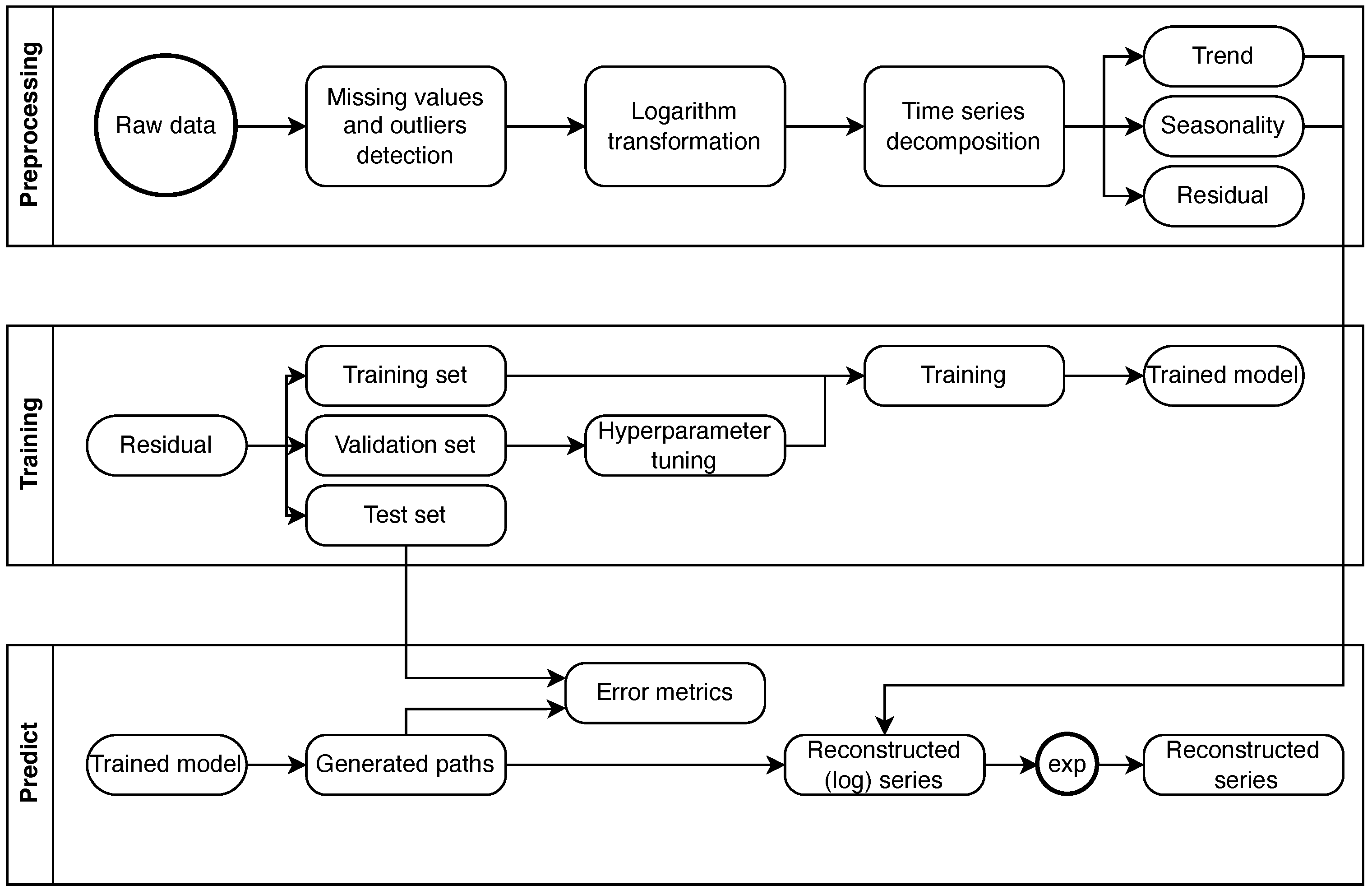
3.1. Data Preprocessing

The dataset comprises a daily time series in which each observation represents the daily average wind energy production in the Italian electricity zone SUD. The dataset spans from 1 January 2015, to 31 December 2021, and it is shown in Figure 3.
The following data preprocessing procedures have been conducted:
  • Missing data and potential outliers have been detected and corrected;
  • The logarithmic transformations have been applied;
  • The series has been decomposed into trends, seasonal and residual components. More specifically, the trend has been obtained via a rolling window smoothing of the series; the analysis of the periodogram allowed to detect the main seasonal component, i.e., annual periodicity, that was successively isolated with a Fourier decomposition; and the residual component has been tested for stationarity; both the Augmented Dickey–Fuller (ADF) test and the Kwiatkowski–Phillips–Schmidt–Shin (KPSS) test confirmed the stationary nature of the residual component.
The residual component was then used to construct the training and test sets for the GAN model. Specifically, each sample point within the data set represents a 7-day-long contiguous segment of the underlying time series. The data from 2015-01-01 to 2020-12-31 are used for training; from 2021-01-01 to 2021-09-30 for validation and hyperparameter tuning; and from 2021-10-01 to 2021-12-31 for testing.

3.2. Model Specification

3.2.1. Software

The PyTorch framework was adopted. The library torchsde [28,55] was used to solve the SDEs, and the library torchcde [52] for its interpolation schemes and to solve the neural CDEs used in the classification and prediction metrics.

3.2.2. Computing Infrastructure

Training was performed on GPU NVIDIA A100 80 GB.

3.2.3. Normalisation

All data were normalised to have zero mean and unit variance.

3.2.4. Architectures

Hyperparameters were selected according to hyperparameter tuning. The Python library ray-tune was used. Every neural network was parametrised as an FFNN with one hidden layer, width 16, and SiLU activations. Every model’s drift, diffusion and vector fields also had a sigmoid nonlinearity as their final operation. The neural SDE’s generator has a hidden state of size x, and the discriminator has a hidden state of size h. These were both taken as x = h = 16 . The Latent ODE, likewise, has an evolving hidden state, which was also taken as size 16. The Latent ODE samples noise from a customarily distributed initial condition, which has been taken to have three dimensions. For the model with fBm, all the hidden sizes and noises were assumed to have dimension one.

3.2.5. Optimisers

The Latent ODE was trained with Adam [56] with a learning rate of 10 3 . The generator and discriminator of the neural SDE were trained with Adadelta, with a learning rate of 0.5 × 10 5 . The learning rates of the model with fBm were chosen to be equal to 10 1 and 0.5 × 10 5 , respectively.

3.2.6. Hurst Index Estimation

One of the pioneering methods for Hurst index estimation is the rescaled range analysis, commonly known as Range over Standard Deviation (R/S). In this section, we will describe the approach mentioned above, and estimate the Hurst index; see [57] for further details.
Generally speaking, this method involves calculating the rescaled range of a time series, which is the difference between the maximum and minimum cumulative sums of data divided by the standard deviation. On the one hand, we remark that the key advantage of R/S analysis lies in its simplicity, making it suitable for initial exploratory analyses; on the other, sensitivity to data size should be taken into account, and adjustments may be necessary for optimal results.

3.3. Algorithm to Estimate H

The approach relies on the representation of the Hurst exponent H in terms of the asymptotic behaviour of the rescaled range as a function of the time span of a time series. Formally:
E R ( n ) S ( n ) = C · n H as n
where:
  • n represents the period of the observations, denoting the number of data points within a time series of length N under consideration;
  • R ( n ) denotes the range of the initial n cumulative deviations from the mean;
  • S ( n ) indicates the range of the series comprising the first n cumulative standard deviations;
  • C is a positive constant.
Therefore, taking into account the cumulative sums of residuals, the following procedure is implemented:
  • For each specified length n { n 1 , , n k = N } , the residuals u = ( u i , i { 1 , , n } ) are extracted from the seasonal decomposition of the observed time series, and the mean u ¯ is subsequently computed;
  • The cumulative deviations are computed as R ^ ( n ) = i = 1 n ( u i u ¯ ) ;
  • The range is computed as max ( R ^ ( n ) ) min ( R ^ ( n ) ) ;
  • S ( n ) is computed as the standard deviation of the cumulative deviations of R ^ ( n ) ;
  • The rescaled ranges are obtained as R ( n ) S ( n ) ;
  • A linear regression of the rescaled ranges is fitted against n on a log scale;
  • H ^ is estimated as the slope of the regression analysis conducted over all the different k lengths considered.

3.4. Data Size Analysis

An R/S analysis was conducted on the residuals, with the optimal data size determined as a result of subsequent analysis:
  • The rolling standard deviation is computed on a yearly basis;
  • Both the minimum and maximum values of the rolling standard deviations are utilised to delineate a grid of five appropriate diffusion coefficients for the fractional Brownian motion. The range spans from the minimum value of 0.7423 to the maximum value of 0.8887, with equal spacing between each coefficient;
  • A grid of nine appropriate values for H is also considered, and it spaces evenly from 0.1 to 0.9;
  • For each combination of H and the diffusion coefficient, we simulate 1000 trajectories for the fBm, over 5 years of daily projections;
  • The calibration algorithm for H is implemented over the trajectories generated using different data size, with RMSE computation realised for each data size selected;
  • The minimum RMSE for H highlights the optimal data size.
The analysis focuses on a specific set of values chosen for their ability to provide deep insights into the model’s dynamics while maintaining simplicity. Although this set may appear limited, each value was meticulously selected to cover a representative spectrum of scenarios and conditions. Expanding the dataset to include more values would not significantly enhance our understanding of the model’s behaviour. Additional values would likely fall within ranges already covered by the selected set, contributing redundant information without introducing meaningful new insights. Furthermore, a denser dataset could obscure significant trends or patterns and overwhelm the reader with excessive data points.
Emphasising a concise yet comprehensive set of values allows for effective assessment of the model’s performance across key metrics, facilitating clear conclusions without unnecessary complexity. This approach maximises the efficiency of our analysis, enabling extraction of valuable insights with minimal noise.
It is noteworthy that the preceding algorithm confirms the optimal window size as the maximum one.
In this specific case, we consider daily residuals across the Italian geographical area of interest, spanning from 1 January 2015, to 31 December 2020.
The algorithm described above produces an the value of H of 0.3522, as showed in Table 1.

3.5. Results

In the simulation methodology, two primary error metrics have been used to assess the performance of the predictive model: Dynamic Time Warping (DTW) and Maximum–Minimum Discrepancy (MMD). These metrics offer distinct perspectives on the accuracy and fidelity of the wind energy production forecasts.
DTW is a technique commonly employed in time series analysis to measure the similarity between two sequences, accounting for variations in the time axis. By aligning the sequences non-linearly, DTW accommodates temporal distortions and fluctuations, making it particularly well-suited for evaluating the performance of time series forecasting models. In other words, DTW measures the degree of correspondence between the predicted and observed energy production trajectories, accounting for potential time shifts and variations.
MMD is a statistical measure used to quantify the dissimilarity between probability distributions. By comparing the maximum difference and minimum difference between the distributions of predicted and observed wind energy production, MMD captures discrepancies in both the mean and variance of the distributions. This metric offers a comprehensive assessment of the model’s predictive accuracy, highlighting deviations in both central tendency and variability.
The implementation of DTW and MMD together provides complementary perspectives on the models’ performance, encompassing both the temporal dynamics and the distributional characteristics of the generated data. Latter metrics allow us to effectively evaluate the quality, accuracy, and consistency of the wind energy production predictions produced by the mentioned models, thus providing a comprehensive assessment of their comparative performance.
The experimental errors are shown in Table 2; they indicate comparable performance for the two models, both with and without the inclusion of fBm.
To better visualise the level of agreement, in Figure 4a and Figure 5a, 50 samples from the true distribution are plotted against 50 from the learned distribution.
The level of agreement between the real and generated distributions is visually assessed by examining the overlap and spread of the trajectories. Both the real and generated trajectories exhibit a comparable spread as they evolve over time, suggesting that the model has effectively learned the variability and stochastic nature of the wind energy production, maintaining a consistent level of divergence comparable to the real data. In addition, the paths of the real and generated trajectories display similar patterns and fluctuations, implying that the model has accurately captured the underlying dynamics and trends of the wind energy production.
In addition to the trajectory comparison, the marginal distributions of the real and generated paths at specific time steps ( t = 1 , 2 , 3 , 4 , 5 ) are presented in Figure 4b and Figure 5b. These histograms provide a more granular view of the model’s performance at each individual time point. The overlap between the real and generated distributions at each time step indicates that the model not only captures the general trend, but also the specific probabilistic characteristics of the data. This overlap reinforces the conclusion that the generated data are statistically similar to the real data. The close agreement between the real and generated distributions at these individual time points underscores the model’s effectiveness in predicting wind energy production.
Since the model has been trained on the residual component of the wind energy production time series, the predictions generated by the model correspond to this residual part. To reconstruct the actual time series of wind energy production, it is necessary to reintroduce the trend and seasonal components that were isolated during the preprocessing steps. Figure 6 shows the recovered time series from the predicted residuals after adding the trend and seasonal components.
Then, the Mean Absolute Percentage Error (MAPE) has been calculated on the recovered time series (in logarithmic form) to assess the accuracy of the model’s predictions. The resulting MAPE value is approximately 13–14%, as shown in Table 3. Although this error rate is not the lowest achievable, it is still within a satisfactory range, indicating that the model performs reasonably well in capturing and predicting the wind energy production dynamics.

4. Conclusions

In this study, predictive models for wind energy production in Italy were applied and evaluated, implementing GANs to capture the stochastic nature of wind behaviour. The investigation aimed to address the challenges associated with precise wind energy prediction, which is crucial for sustainable energy planning and management.
Through extensive numerical simulations and analyses, the effectiveness of the proposed approach in accurately forecasting wind energy production has been demonstrated. By treating the wind energy production time series as a realisation of a stochastic process, the complex dynamics and uncertainties inherent in wind generation have been successfully modelled.
Despite the introduction of fBm, comparable errors were observed between the two models.
This can be attributed to the linear transformation (4) that may mitigate the contribution of the fBm, resulting in similar error profiles between the models. The observed limited impact may be attributed to the consideration of fBm with dimensionality restricted to 1. Future research could explore the generalisation of the generation algorithm for fBm to encompass higher dimensions, as well as other models for characterising long-range dependency, such as the fractional Lévy stable motion (fLsm). With two parameters, α and H, the latter could characterise local irregularity and global persistence separately.

Author Contributions

Conceptualisation, L.D.P., N.F. and A.V.; methodology, L.D.P., N.F. and A.V.; software, N.F. and A.V.; validation, L.D.P., N.F. and A.V.; formal analysis, L.D.P., N.F. and A.V.; investigation, L.D.P., N.F. and A.V.; resources, A.V.; data curation, N.F. and A.V.; writing—original draft preparation, L.D.P., N.F. and A.V.; writing—review and editing, L.D.P., N.F. and A.V.; visualisation, L.D.P., N.F. and A.V.; supervision, L.D.P.; project administration, L.D.P., N.F. and A.V.; funding acquisition, N.F. All authors have read and agreed to the published version of the manuscript.

Funding

This research was realised with co-financing of the European Union—NOP Research and Innovation 2014–2020.

Data Availability Statement

Data sharing not applicable. No new data were created or analysed in this study. Data sharing is not applicable to this article.

Conflicts of Interest

The authors declare no conflicts of interest.

Abbreviations

The following abbreviations are used in this manuscript:
ARMAAutoregressive moving average
CGANConditional GAN
CNNConvolutional neural network
CSEControlled differential equation
DTWDynamic Time Warping
fBmFractional Brownian motion
FFNNFeedforward neural network
fLsmFractional Lévy stable motion
GANGenerative adversarial network
GAN-GPGAN with gradient penalty
MAPEMean absolute percentage error
MMDMaximum–Minimum Discrepancy
NNNeural networks
SDEStochastic differential equation
SeqGANSequence GAN
VAEVariational autoencoder
WGANWasserstein GAN

References

  1. Zhang, X.; Ma, C.; Song, X.; Zhou, Y.; Chen, W. The impacts of wind technology advancement on future global energy. Appl. Energy 2016, 184, 1033–1037. [Google Scholar] [CrossRef]
  2. Commission, E. Clean Energy. 2019. Available online: https://ec.europa.eu/commission/presscorner/detail/en/fs_19_6723 (accessed on 18 May 2024).
  3. Weron, R. Modeling and Forecasting Electricity Loads and Prices: A Statistical Approach; John Wiley & Sons: Hoboken, NJ, USA, 2006; Volume 396. [Google Scholar]
  4. Di Persio, L.; Fraccarolo, N. Energy consumption forecasts by gradient boosting regression trees. Mathematics 2023, 11, 1068. [Google Scholar] [CrossRef]
  5. Di Persio, L.; Fraccarolo, N. Investment and Bidding Strategies for Optimal Transmission Management Dynamics: The Italian Case. Energies 2023, 16, 5950. [Google Scholar] [CrossRef]
  6. Foley, A.M.; Leahy, P.G.; Marvuglia, A.; McKeogh, E.J. Current methods and advances in forecasting of wind power generation. Renew. Energy 2012, 37, 1–8. [Google Scholar] [CrossRef]
  7. Hu, J.; Heng, J.; Wen, J.; Zhao, W. Deterministic and probabilistic wind speed forecasting with de-noising-reconstruction strategy and quantile regression based algorithm. Renew. Energy 2020, 162, 1208–1226. [Google Scholar] [CrossRef]
  8. Wang, Y.; Li, Y.; Zou, R.; Foley, A.M.; Al Kez, D.; Song, D.; Hu, Q.; Srinivasan, D. Sparse heteroscedastic multiple spline regression models for wind turbine power curve modeling. IEEE Trans. Sustain. Energy 2020, 12, 191–201. [Google Scholar] [CrossRef]
  9. Yunus, K.; Thiringer, T.; Chen, P. ARIMA-based frequency-decomposed modeling of wind speed time series. IEEE Trans. Power Syst. 2015, 31, 2546–2556. [Google Scholar] [CrossRef]
  10. Kavasseri, R.G.; Seetharaman, K. Day-ahead wind speed forecasting using f-ARIMA models. Renew. Energy 2009, 34, 1388–1393. [Google Scholar] [CrossRef]
  11. Maatallah, O.A.; Achuthan, A.; Janoyan, K.; Marzocca, P. Recursive wind speed forecasting based on Hammerstein Auto-Regressive model. Appl. Energy 2015, 145, 191–197. [Google Scholar] [CrossRef]
  12. Wang, J.; Wang, S.; Yang, W. A novel non-linear combination system for short-term wind speed forecast. Renew. Energy 2019, 143, 1172–1192. [Google Scholar] [CrossRef]
  13. Wang, Y.; Wang, J.; Wei, X. A hybrid wind speed forecasting model based on phase space reconstruction theory and Markov model: A case study of wind farms in northwest China. Energy 2015, 91, 556–572. [Google Scholar] [CrossRef]
  14. Liu, H.; Mi, X.; Li, Y. Smart multi-step deep learning model for wind speed forecasting based on variational mode decomposition, singular spectrum analysis, LSTM network and ELM. Energy Convers. Manag. 2018, 159, 54–64. [Google Scholar] [CrossRef]
  15. Song, J.; Wang, J.; Lu, H. A novel combined model based on advanced optimization algorithm for short-term wind speed forecasting. Appl. Energy 2018, 215, 643–658. [Google Scholar] [CrossRef]
  16. He, X.; Nie, Y.; Guo, H.; Wang, J. Research on a Novel Combination System on the Basis of Deep Learning and Swarm Intelligence Optimization Algorithm for Wind Speed Forecasting. IEEE Access 2020, 8, 51482–51499. [Google Scholar] [CrossRef]
  17. Mezaache, H.; Bouzgou, H. Auto-Encoder with Neural Networks for Wind Speed Forecasting. In Proceedings of the 2018 International Conference on Communications and Electrical Engineering (ICCEE), El Oued, Algeria, 17–18 December 2018; pp. 1–5. [Google Scholar] [CrossRef]
  18. Fu, W.; Wang, K.; Tan, J.; Zhang, K. A composite framework coupling multiple feature selection, compound prediction models and novel hybrid swarm optimizer-based synchronization optimization strategy for multi-step ahead short-term wind speed forecasting. Energy Convers. Manag. 2020, 205, 112461. [Google Scholar] [CrossRef]
  19. Niu, Z.; Yu, Z.; Tang, W.; Wu, Q.; Reformat, M. Wind power forecasting using attention-based gated recurrent unit network. Energy 2020, 196, 117081. [Google Scholar] [CrossRef]
  20. Yu, Y.; Han, X.; Yang, M.; Yang, J. Probabilistic Prediction of Regional Wind Power Based on Spatiotemporal Quantile Regression. In Proceedings of the 2019 IEEE Industry Applications Society Annual Meeting, Baltimore, MD, USA, 29 September–3 October 2019; pp. 1–16. [Google Scholar] [CrossRef]
  21. Kosovic, B.; Haupt, S.E.; Adriaansen, D.; Alessandrini, S.; Wiener, G.; Delle Monache, L.; Liu, Y.; Linden, S.; Jensen, T.; Cheng, W.; et al. A comprehensive wind power forecasting system integrating artificial intelligence and numerical weather prediction. Energies 2020, 13, 1372. [Google Scholar] [CrossRef]
  22. Liu, T.; Huang, Z.; Tian, L.; Zhu, Y.; Wang, H.; Feng, S. Enhancing wind turbine power forecast via convolutional neural network. Electronics 2021, 10, 261. [Google Scholar] [CrossRef]
  23. Shi, J.; Guo, J.; Zheng, S. Evaluation of hybrid forecasting approaches for wind speed and power generation time series. Renew. Sustain. Energy Rev. 2012, 16, 3471–3480. [Google Scholar] [CrossRef]
  24. Chen, C.; Liu, H. Dynamic ensemble wind speed prediction model based on hybrid deep reinforcement learning. Adv. Eng. Informatics 2021, 48, 101290. [Google Scholar] [CrossRef]
  25. Chen, Y.; Zhang, S.; Zhang, W.; Peng, J.; Cai, Y. Multifactor spatio-temporal correlation model based on a combination of convolutional neural network and long short-term memory neural network for wind speed forecasting. Energy Convers. Manag. 2019, 185, 783–799. [Google Scholar] [CrossRef]
  26. Chen, J.; Zeng, G.Q.; Zhou, W.; Du, W.; Lu, K.D. Wind speed forecasting using nonlinear-learning ensemble of deep learning time series prediction and extremal optimization. Energy Convers. Manag. 2018, 165, 681–695. [Google Scholar] [CrossRef]
  27. Wang, G.; Jia, R.; Liu, J.; Zhang, H. A hybrid wind power forecasting approach based on Bayesian model averaging and ensemble learning. Renew. Energy 2020, 145, 2426–2434. [Google Scholar] [CrossRef]
  28. Kidger, P.; Foster, J.; Li, X.; Lyons, T.J. Neural SDEs as Infinite-Dimensional GANs. In Proceedings of the Proceedings of the 38th International Conference on Machine Learning, Virtual, 18–24 July 2021; Volume 139. [Google Scholar]
  29. Goodfellow, I.; Pouget-Abadie, J.; Mirza, M.; Xu, B.; Warde-Farley, D.; Ozair, S.; Courville, A.; Bengio, Y. Generative adversarial nets. Adv. Neural Inf. Process. Syst. 2014, 27, 2672–2680. [Google Scholar]
  30. Zhu, J.Y.; Park, T.; Isola, P.; Efros, A.A. Unpaired Image-to-Image Translation Using Cycle-Consistent Adversarial Networks. In Proceedings of the 2017 IEEE International Conference on Computer Vision (ICCV), Venice, Italy, 22–29 October 2017; pp. 2242–2251. [Google Scholar] [CrossRef]
  31. Yuan, R.; Wang, B.; Mao, Z.; Watada, J. Multi-objective wind power scenario forecasting based on PG-GAN. Energy 2021, 226, 120379. [Google Scholar] [CrossRef]
  32. Chen, Y.; Wang, Y.; Kirschen, D.; Zhang, B. Model-Free Renewable Scenario Generation Using Generative Adversarial Networks. IEEE Trans. Power Syst. 2018, 33, 3265–3275. [Google Scholar] [CrossRef]
  33. Chen, Y.; Li, P.; Zhang, B. Bayesian renewables scenario generation via deep generative networks. In Proceedings of the 2018 52nd Annual Conference on Information Sciences and Systems (CISS), Princeton, NJ, USA, 13–15 March 2018; pp. 1–6. [Google Scholar] [CrossRef]
  34. Jiang, C.; Mao, Y.; Chai, Y.; Yu, M.; Tao, S. Scenario Generation for Wind Power Using Improved Generative Adversarial Networks. IEEE Access 2018, 6, 62193–62203. [Google Scholar] [CrossRef]
  35. Wei, H.; Hongxuan, Z.; Yu, D.; Yiting, W.; Ling, D.; Ming, X. Short-term optimal operation of hydro-wind-solar hybrid system with improved generative adversarial networks. Appl. Energy 2019, 250, 389–403. [Google Scholar] [CrossRef]
  36. Chen, Y.; Wang, X.; Zhang, B. An Unsupervised Deep Learning Approach for Scenario Forecasts. In Proceedings of the 2018 Power Systems Computation Conference (PSCC), Dublin, Ireland, 11–15 June 2018; pp. 1–7. [Google Scholar] [CrossRef]
  37. Wang, F.; Zhang, Z.; Liu, C.; Yu, Y.; Pang, S.; Duić, N.; Shafie-khah, M.; Catalão, J.P. Generative adversarial networks and convolutional neural networks based weather classification model for day ahead short-term photovoltaic power forecasting. Energy Convers. Manag. 2019, 181, 443–462. [Google Scholar] [CrossRef]
  38. Zhang, Y.; Ai, Q.; Xiao, F.; Hao, R.; Lu, T. Typical wind power scenario generation for multiple wind farms using conditional improved Wasserstein generative adversarial network. Int. J. Electr. Power Energy Syst. 2020, 114, 105388. [Google Scholar] [CrossRef]
  39. Liang, J.; Tang, W. Sequence Generative Adversarial Networks for Wind Power Scenario Generation. IEEE J. Sel. Areas Commun. 2020, 38, 110–118. [Google Scholar] [CrossRef]
  40. Sun, Z.; El-Laham, Y.; Vyetrenko, S. Neural Stochastic Differential Equations with Change Points: A Generative Adversarial Approach. In Proceedings of the ICASSP 2024–2024 IEEE International Conference on Acoustics, Speech and Signal Processing (ICASSP), Seoul, Republic of Korea, 14–19 April 2024; IEEE: Piscataway, NJ, USA, 2024; pp. 6965–6969. [Google Scholar]
  41. Allouche, M.; Girard, S.; Gobet, E. A generative model for fBm with deep ReLU neural networks. J. Complex. 2022, 73, 101667. [Google Scholar] [CrossRef]
  42. Oksendal, B. Stochastic Differential Equations: An Introduction with Applications; Springer Science & Business Media: Berlin/Heidelberg, Germany, 2013. [Google Scholar]
  43. Rogers, L.C.G.; Williams, D. Diffusions, Markov Processes and Martingales: Volume 2, Itô Calculus; Cambridge University Press: Cambridge, UK, 2000; Volume 2. [Google Scholar]
  44. Chen, R.T.; Rubanova, Y.; Bettencourt, J.; Duvenaud, D.K. Neural ordinary differential equations. Adv. Neural Inf. Process. Syst. 2018, 31. [Google Scholar]
  45. Kidger, P.; Morrill, J.; Foster, J.; Lyons, T. Neural Controlled Differential Equations for Irregular Time Series. In Proceedings of the Advances in Neural Information Processing Systems, Online, 6–12 December 2020; Larochelle, H., Ranzato, M., Hadsell, R., Balcan, M., Lin, H., Eds.; Curran Associates, Inc.: Glasgow, UK, 2020; Volume 33, pp. 6696–6707. [Google Scholar]
  46. Kidger, P. On neural differential equations. arXiv 2022, arXiv:2202.02435. [Google Scholar]
  47. Yang, L.; Gao, T.; Lu, Y.; Duan, J.; Liu, T. Neural network stochastic differential equation models with applications to financial data forecasting. Appl. Math. Model. 2022, 115, 279–299. [Google Scholar] [CrossRef]
  48. Kong, L.; Sun, J.; Zhang, C. Sde-net: Equipping deep neural networks with uncertainty estimates. arXiv 2020, arXiv:2008.10546. [Google Scholar]
  49. Gierjatowicz, P.; Sabaté-Vidales, M.; Šiška, D.; Szpruch, Ł.; Zuric, Z. Robust pricing and hedging via neural stochastic differential equations. J. Comput. Financ. 2022, 16. [Google Scholar] [CrossRef]
  50. Veeravalli, T.; Raginsky, M. Nonlinear controllability and function representation by neural stochastic differential equations. arXiv 2022, arXiv:2212.00896. [Google Scholar] [CrossRef]
  51. Yang, L.; Zhang, D.; Karniadakis, G. Physics-Informed Generative Adversarial Networks for Stochastic Differential Equations. SIAM J. Sci. Comput. 2018, 42, A292–A317. [Google Scholar] [CrossRef]
  52. Kidger, P.; Morrill, J.; Foster, J.; Lyons, T. Neural controlled differential equations for irregular time series. Adv. Neural Inf. Process. Syst. 2020, 33, 6696–6707. [Google Scholar]
  53. Arjovsky, M.; Chintala, S.; Bottou, L. Wasserstein generative adversarial networks. In Proceedings of the International Conference on Machine Learning, PMLR, Sydney, Australia, 6–11 August 2017; pp. 214–223. [Google Scholar]
  54. Gulrajani, I.; Ahmed, F.; Arjovsky, M.; Dumoulin, V.; Courville, A.C. Improved training of wasserstein gans. Adv. Neural Inf. Process. Syst. 2017, 30. [Google Scholar]
  55. Li, X.; Wong, T.K.L.; Chen, R.T.Q.; Duvenaud, D. Scalable gradients for stochastic differential equations. In Proceedings of the Twenty Third International Conference on Artificial Intelligence and Statistics (AISTATS), Online, 26–28 August 2020. [Google Scholar]
  56. Kingma, D.P.; Ba, J. Adam: A Method for Stochastic Optimization. arXiv 2017, arXiv:1412.6980. [Google Scholar]
  57. Qian, B.; Rasheed, K. Hurst exponent and financial market predictability. In Proceedings of the IASTED Conference on Financial Engineering and Applications, Cambridge, MA, USA, 8–10 November 2007; pp. 203–209. [Google Scholar]
Figure 1. (Left): distribution of wind energy production in Italy. (Right): wind power capacity (GW) from 2013 to 2024. Source: Terna.
Mathematics 12 02105 g001
Figure 2. Flowchart representing the steps from raw data to the forecasting of wind energy.
Mathematics 12 02105 g002
Figure 3. Time series of the daily average wind energy production in SUD zone.
Mathematics 12 02105 g003
Figure 4. (a) Sample paths from the real and the generated processes. (b) Left to right: marginal distributions at t = 1 , 2 , 3 , 4 , 5 .
Mathematics 12 02105 g004
Figure 5. (a) Sample paths from the real and the generated processes for the model with fBm. (b) Left to right: marginal distributions at t = 1 , 2 , 3 , 4 , 5 for the model with fBm.
Mathematics 12 02105 g005
Figure 6. (a) Actual versus predicted wind energy production (in log scale). (b) Actual versus predicted wind energy production with fBm (in log scale).
Mathematics 12 02105 g006
Table 1. Estimation results for the Hurst exponent.
Zone H ^
SUD0.3522
Table 2. Experimental results.
MetricNeural SDENeural SDE with fBm
DTW3.30783.0743
MMD0.10420.1091
Table 3. MAPE (%) computed on the reconstructed time series after adding trend and seasonality.
MetricNeural SDENeural SDE with fBm
MAPE13.4014.29
Disclaimer/Publisher’s Note: The statements, opinions and data contained in all publications are solely those of the individual author(s) and contributor(s) and not of MDPI and/or the editor(s). MDPI and/or the editor(s) disclaim responsibility for any injury to people or property resulting from any ideas, methods, instructions or products referred to in the content.

