Software Fault Localization Based on Weighted Association Rule Mining and Complex Networks

Abstract

Software fault localization technology aims to identify suspicious statements that cause software failures, which is crucial for ensuring software quality. Spectrum-based software fault location (SBFL) technology calculates the suspiciousness of each statement by analyzing the correlation between statement coverage information and execution results in test cases. SBFL has attracted increasing attention from scholars due to its high efficiency and scalability. However, existing SBFL studies have shown that a large number of statements share the same suspiciousness, which hinders software debuggers from quickly identifying the location of faulty statements. To address this challenge, we propose an SBFL model based on weighted association rule mining and complex networks: FL-WARMCN. The algorithm first uses Jaccard to measure the distance between passing and failing test cases, and applies it as the weight of passing test cases. Next, FL-WARMCN calculates the initial suspiciousness of each statement based on the program spectrum data. Then, the FL-WARMCN model utilizes a weighted association rule mining algorithm to obtain the correlation relationships between statements and models the network based on this. In the network, the suspiciousness of statements is used as node weights, and the correlation between statements is used as edge weights. We chose the eigenvector centrality that takes into account the degree centrality of statements and the importance of neighboring statements to calculate the importance of each statement, and used it as a weight to incorporate into the weighted suspiciousness calculation of the statement. Finally, we applied the FL-WARMCN model for experimental validation on the Defects4J dataset. The results showed that the model was significantly superior to other baselines. In addition, we analyzed the impact of different node and edge weights on model performance.

1. Introduction

With the increasing complexity and scale of software systems, the existence of software faults can lead to irreparable damage, particularly in safety-critical software. However, software debugging is widely acknowledged as a time-consuming and labor-intensive challenge, requiring developers to invest significant effort. During this process, software debuggers manually inspect program elements to find the exact location of a fault. To alleviate this pressure, researchers have shown considerable interest in spectrum-based fault localization (SBFL) technology due to its high efficiency [1]. SBFL offers several advantages, including language independence, comprehensibility, and ease of computation [2].

SBFL technology utilizes the results of test case execution and the coverage information of each code statement in the test case as input. It applies statistical analysis techniques to evaluate the likelihood of statement failure, which also indicates the suspiciousness of each statement. The underlying principle is that a statement is considered more suspicious if it appears more frequently in failed test cases compared to passed test cases. The output of SBFL is a ranking of all statements based on their suspiciousness, with more suspicious elements listed first. This allows software debuggers to efficiently identify the location of faults. Common SBFL methods include Barinel [3], Ochiai [4], Dstar [5], and Tarantula [6].

Elements tie [2,7] is a significant challenge in SBFL research, which refers to a large number of statements being assigned the same suspiciousness, resulting in many ties in the final ranking of fault statements. Therefore, software debuggers have to check all statements with the same ranking to determine the location of the fault, especially when there are many statements with the same ranking, which greatly restricts the efficiency of software debugging. The reason for this is that existing SBFL methods mainly rely on the correlation between statement coverage information and test case execution results for calculation, which leads to the sharing of the same suspiciousness among code within a program block [8]. To eliminate this negative impact, researchers have explored the incorporation of additional information into SBFL, including code metrics [9], mutation analysis [10], and development history [11]. Code metrics quantify some characteristic attributes of software source code, but they lack the granularity to evaluate each statement effectively. The development history may not always provide valuable code information in practical scenarios, and mutation analysis is a highly time-consuming task. Therefore, it is not feasible to integrate additional information in SBFL, and researchers have begun to focus on increasing the distinction between statements by introducing statement importance and test case importance.

In terms of statement importance, existing SBFL research based on deep learning [9,12,13,14,15,16] aims to learn the nonlinear relationship between sentences and defects. Wang et al. [9] proposed a fault localization method by wide&deep learning on multiple groups of features (W&DFL), which combines seven features: spectrum-based suspiciousness, mutation-based suspiciousness, behavior-based suspiciousness, variables-based suspiciousness, stack trace of crash, static metrics, and invariant changes. The combination of these features effectively improves the fault localization performance of the model. Similarly, DeepFL [13] integrates multidimensional fault diagnosis information and utilizes deep learning to automatically identify the most useful features for precise fault localization. In addition, this study investigated the impact of different deep learning model configurations and parameters on the performance of DeepFL. The GNet4FL model [16] has been proposed. This model first combines the static features of the program code with the dynamic features of the test results, and uses GraphSAGE to obtain node representations in the program code to preserve topological information. Finally, the program entities are sorted using a multi-layer perceptron (MLP) to improve the accuracy of software fault localization. Although the aforementioned SBFL research based on deep learning has shown that more effective differentiation of statements (elements) can improve fault localization performance [12], the high computational cost of deep learning is not conducive to practical engineering applications and promotion.

Inspired by this, researchers are committed to characterizing the relationships between statements through network structures and calculating the importance of statements through complex network theory, thereby increasing the discrimination between statements [17,18]. There are also many interrelated factors in the software source code, which has led to the research of combining complex network theory with SBFL technology. A fault localization method based on complex network theory, FLCN [19], has been proposed. FLCN first constructs a network framework based on the code coverage information of all test cases and obtains the relationships between statements through the generated network structure. Each statement is represented as a node, and the execution relationships of the statements contained in the test cases are represented as edges. Finally, this method calculates the degree centrality (DC) and proximity centrality (CC) of each statement separately and uses DC-CC as the degree of doubt for each statement. On this basis, a single fault localization method FLCN-S [20] based on complex network theory is proposed. The main difference between this method and FLCN is that it only extracts the code coverage information of failed test cases to construct a network framework. Zhu et al. [21] proposed a fault localization method based on software network centrality measures (SNCM). This algorithm first constructs a software network by treating statements as network nodes and the execution relationships between statements as edges of the network. Then, SNCM utilizes centrality measures in complex network theory to calculate statement importance and calculates the degree and burst coefficient for each node (statement) separately. Finally, it calculates statements’ suspiciousness based on degree and burst coefficient. However, the above research only considered the importance of target statements and the correlation between statements, but ignored the importance of target-related statements. The study by He et al. [22] has confirmed that if the target statement is more likely to trigger a fault, the statements in the test case that are more relevant to the target statement are more likely to be suspected. Therefore, it is necessary to incorporate the importance of relevant statements into the calculation of statement importance while considering the relationships between statements. Regarding the issue of elements tie, although the above research introduces statement importance, it overlooks the potential impact of related statement importance on the suspiciousness of the target statement.

In terms of test case importance, classic SBFL methods (such as Barinel [3], Ochiai [4], etc.) calculate the suspicious score of statements based on the proportion of the number of failed and passed test cases, but they all assume that all test cases are equally important. However, test cases are not equally important, for example, passed test cases that are similar to failed test cases are more conducive to analyzing the location of fault statements. In addition, existing research has confirmed that adding weights to test cases is beneficial for alleviating elements tie and improving the performance of fault locators [23,24,25]. Bandyopadhyay et al. [23] uses the heuristic method of the extended nearest neighbor model to calculate test case weights. Specifically, the nearest neighbor model is used to calculate the difference in statement coverage between failed and passed test cases. In addition, this method measures the closeness between each passing test case and all failed test cases. The PRFL model [26] is proposed, which assigns weights to different test cases through PageRank. PRFL first constructs a dynamic call graph between methods. Then, the algorithm generates weighted program spectrum information by constructing a connection matrix between the test and the method. Finally, the weighted program spectrum is used as input for PRFL and the fault statements are sorted using the existing suspiciousness formula. Yang et al. [25] applied cosine similarity to measure the similarity between test cases, providing a basis for similarity weighting. The similarity weighting method was applied to various common fault localization algorithms (such as Barinel [3], Tarantula [6], etc.), and it was experimentally verified that this method effectively improves localization efficiency. The above research has indeed alleviated the problem of elements tie, but by weighting test cases, it only increases the discrimination of statements under different test case coverage. Unfortunately, statements that appear simultaneously in the same test case still share the same suspiciousness, and the issue of elements tie has not been completely resolved.

In summary, according to our research, existing SBFL studies have not yet considered both statement importance and test case importance to increase sentence discrimination. Therefore, our research motivation is to design an SBFL method that combines high performance and comprehensibility, while considering both the importance of test cases and statements, to solve the problem of elements tie. We propose an SBFL model based on weighted association rule mining and complex networks, named FL-WARMCN. It first calculates the similarity between passing and failing test cases according to the Jaccard metric to determine the importance (weight) of each test case. Then, the Weighted Association Rule Mining (WARM) algorithm serves as the link between the importance of test cases and the importance of statements in the FL-WARMCN model. By converting weighted test case data into weighted transaction data, the WARM algorithm is used to obtain the correlation between statements, preparing for the construction of networks. Next, we model the network based on all associated relationships, which characterizes the importance of the statement itself and the complex relationships between statements. In the network, statements are used as nodes and suspiciousness is applied as the weight of each node. Accuracy is assigned as edge weight, and the eigenvector centrality is used to represent the importance of each node. Finally, FL-WARMCN integrates the node importance into the corresponding statement suspiciousness to sort all the statements and outputs the sorting result of the faulty statement. The main contributions of this paper are summarized as follows:

(1)

FL-WARMCN assigns different weights to test cases and utilizes complex networks to obtain the importance of statements. By simultaneously considering the importance of test cases and statements, it enhances the differentiation of statements to break the elements tie.

(2)

FL-WARMCN visualizes the complex relationships between statements by modeling a network. It also takes into account the correlation between the target and related statements, and the importance of related statements through the eigenvector centrality.

(3)

We conducted experimental comparisons between FL-WARMCN and five baseline algorithms on 10 datasets of Defects4J. The results demonstrated that this algorithm outperformed the optimal baseline, with an improvement of 8.29% in the EXAM score and 18.31% in the MWE.

The remaining sections of this article are organized as follows: Section 2 describes the FL-WARMCN model, including the model framework, use case importance calculation, statement importance calculation, and fault location method. We list the detailed experimental content in Section 3, including the research questions, experimental subjects, evaluation metrics, and results analysis. Section 4 analyzes the improvement of the FL-WARMCN model in fault location capabilities through quantity and accuracy. Section 5 analyzes the validity of this study. Section 6 concludes the article and discusses future work.

2. Materials and Methods

This section introduces the FL-WARMCN model, specifically including the overview of FL-WARMCN, test case importance calculation, statement importance calculation, and fault localization method. Additionally, a motivating example is provided to aid comprehension.

2.1. Overview of FL-WARMCN

The association rule mining (ARM) algorithm is dedicated to exploring the correlation between variables hidden in a large amount of data, and the complex network theory is applied to express the characteristics and relationships of variables in complex systems. Therefore, the integration of ARM and complex network theory is appropriate, and existing studies [27,28,29,30] also show the application effectiveness of the combination of these two techniques. Under this motivation, we propose FL-WARMCN, and the overall research framework is shown in Figure 1. This method first considers the importance of test cases and adopts Jaccard to assign different weights to different transactions (test cases); then, we apply the WARM algorithm to mine association relationships (association rules) between statements. After FL-WARMCN obtains all the association rules, it takes the items (antecedents and consequents) in association rules as the nodes of the complex networks, the suspiciousness as the node weight, the association rules as the edge, and the Accuracy as the edge weight to construct an undirected weighted network. Finally, the eigenvector centrality is applied to express the importance of statements and used as a weight to calculate the suspiciousness of statements. The calculation results are sorted in descending order as the result of fault statements.

The construction process of the FL-WARMCN model is presented in Algorithm 1. The input consists of the spectrum S of the given software program and the parameters required by WARM: the maximum length of frequent itemsets $MaxLen$, the minimum support threshold $Sup$, and the minimum confidence threshold $Conf$. Lines 1–4 involve creating a dictionary to store weights and suspiciousness. In line 5, the FL-WARMCN model converts the program spectrum S into transactional data for subsequent processing in complex networks. We iterate through the transactional data and utilize Jaccard to quantify the weight of each transaction (test case), as shown in lines 6–7. Line 8 explains that WARM is employed to extract the correlation between statements and between statements and faults from weighted transactional data, based on the predefined $Sup$ and $Conf$ set by the user. In line 9, we calculate the initial suspiciousness of each statement by considering the association relationships between the statement and the fault, and store it in the $Susp$ dictionary. Lines 10–11 demonstrate the utilization of the relationships between statements in constructing complex networks, where the association relationships represent the edge weight, the correlation represents the edge weight, and the node weight is determined by the suspiciousness. Subsequently, we employ eigenvector centrality to determine the importance of each statement. The FL-WARMCN model considers the statement’s importance and initial suspiciousness to determine the final suspiciousness of each statement. Finally, the statements are sent to the software debugger in descending order of their final suspiciousness, as depicted in lines 12–15.

Algorithm 1: Pseudo-code of FL-WARMCN model

Inputs: program spectrum S, maximum length of frequent itemsets $MaxLen$, support  threshold $Sup$, and confidence threshold $Conf$;  Outputs: ranked list of statement suspiciousness $Lis{t}_R$;  1 $MaxLen=2$; /* maximum length of frequent itemsets is set to 2 */  2 $Sup=0$;/* support threshold is set to 0 */  3 $Conf=0$;/* confidence threshold is set to 0 */  4 $W_T,W_S,Susp=dict\left(\right)$;/* create transaction weights, statement weights, and suspiciousness  dictionaries, respectively. */  5 $T=Convert\text{\_}to\text{\_}transaction(S$);  6 $\mathbf{for}$ C in $\mathbf{range}\left(\mathbf{len}\right(T\left)\right)$:  7   $W_T\left[t\right]=\frac{t\cap T_F}{t\cup T_F}$;/* test case importance calculation */  8 $R=Wapriori(T,W_T,Sup,Conf)$;/* generate rules through weighted association rule mining */  9 $Susp=Calculate\text{\_}suspiciousness\left(R\right)$;  10 $N=Generate\text{\_}complex\text{\_}networks\left(R\right)$;  11 $W_S=Calculate\text{\_}eigenvector\text{\_}centrality\left(N\right)$;  12 $\mathbf{for}$ $statement$ in P:/*iterate over each statement in the given program*/  13    $Susp\left[statement\right]=W_S\left[statement\right]\ast Susp\left[statement\right]$;  14 $Lis{t}_R=\mathbf{sorted}(Susp.items\left(\right),\mathbf{key}=lambdax:x\left[1\right],\mathbf{reverse}=\mathbf{True})$  15 $\mathbf{return}Lis{t}_R$

2.2. Test Case Importance Calculation

ARM [31] is applied to explore hidden and meaningful patterns from massive data, and the basic form of association rules is $X\Rightarrow Y$. Among them, X and Y, respectively, represent the antecedent and the consequent of an association rule, which means that if X occurs, Y occurs. We have a transactional dataset T=$\{t_1,t_2,t_3,\dots ,t_M\}$, where t represents each transaction and M represents the amount of transaction data. In SBFL research, t represents test cases and M represents the total number of test cases. We have an n-itemset $I_N$=$\{i_1,i_2,i_3,\dots ,i_N\}$, where i represents each item and N represents the number of items in the itemset. In the SBFL task, i represents each statement and N represents the number of statements in the itemset. The basic flow of the ARM algorithm is to first calculate its support from the 1-itemset in transactions, as shown in Equation (1):

$$Support\left(I_N\right)=\frac{Count\left(I_N\right)}{M}$$

(1)

In the above formula, Count($I_N$) indicates the number of transactions (test cases) including $I_N$. Next, the 1-itemsets that meet the support threshold (user assignment) are converted into frequent 1-itemsets, and the candidate 2-itemsets are obtained by pairwise combination of frequent 1-itemsets. Candidate 2-itemsets that meet the support threshold are converted into frequent 2-itemsets. According to this process, the number of itemsets has accumulated until there are no itemsets higher than the support threshold, and the algorithm stops. After obtaining all the frequent itemsets, ARM converts the frequent itemsets into association rules according to the confidence, as shown in Equation (2):

$$Confidence(X\Rightarrow Y)=\frac{Support(X\cup Y)}{Support\left(X\right)}$$

(2)

A major limitation of traditional ARM is its assumption that all items or transactions are equally important [32]. However, in the context of SBFL research, test cases are not equally significant. Faults are more likely to occur in statements within failing test cases, indicating that failing test cases are more strongly correlated with software failures and, therefore, they hold greater importance than passing test cases. Recognizing the significance of transactions, researchers have increasingly focused on WARM, which employs the transaction weighting strategy. Sun et al. [33] proposed a WARM method based on transaction weighting, called Link-Based Association Rule Mining. It calculates the importance of transaction data through a link-based model. The basic idea is that more important transactions contain more important items. This method describes the relationship between transaction data and items through the bipartite graph and applies Kleinberg’s HITS model [34] to calculate transaction weights, and obtains the central weight of all transactions when the HITS model converges. Experimental results show that this approach can mine some itemsets with low frequency but high quality based on emphasizing the importance of transactions. FICLV [35] is a weighted frequent itemset mining method with customer lifetime value (CLV) as transaction weight to mine customer value. FICLV first calculates the CLV of each consumer and adds it to the corresponding transaction, then filters out frequent itemsets through CLV-weighted support, and finally generates high-quality association rules. FICLV has been fully experimentally verified on the HC-POS dataset. The results demonstrate the effectiveness of the FICLV algorithm and find that it can explore more valuable patterns than the traditional ARM algorithm. Weighted Patient Data Analyzer (WeP-DatA) [32] is applied to mine weighted association rules in weighted data. WeP-DatA adopts the number and tf-idf of prescriptions as the weight of transactions, and uses weighted support and weighted confidence to generate the rule set to explore valuable medical domain knowledge. This algorithm has been verified on a dataset of diabetic patients, and the results prove that the patterns obtained by WeP-DatA are consistent with relevant disease guidelines and are beneficial to the analysis of patient data.

To summarize, the aforementioned research demonstrates that the WARM algorithm, which assigns transaction importance as the weight, is more effective in uncovering valuable association relationships. However, to the best of our knowledge, current fault localization techniques do not utilize the WARM algorithm to investigate the correlation between variables.

As depicted in Figure 1, FL-WARMCN initially generates a program spectrum through statement coverage information and execution results of test cases. In the program spectrum, 0 and 1 indicate the coverage information of each statement in the test case. Specifically, 0 signifies that the statement does not cover the test case, while 1 indicates that the statement covers the test case. The terms Pass and Fail denote the two execution results of the test case. For the application of the WARM algorithm, we convert program spectrum information into transactional data. Transactional data only show the statements that exist in the test case (the statement with 1 in the program spectrum): a test case represents a transaction and a statement represents an item. For instance, Equation (3) represents the program spectrum while Equation (4) represents the corresponding transactional data. $Tran{s}_{P1}$ and $Tran{s}_{F1}$ are the identifiers of the transactions. The transaction data consist of statements and test case execution results, where each statement or test case execution result represents an item.

$$\left[\begin{array}{cccccc}1& 0& 0& 1& 1& 1\\ 1& 0& 1& 1& 0& 1\end{array}\right]\left[\begin{array}{c}\mathrm{P}\\ \mathrm{F}\end{array}\right]$$

(3)

$$\left[\begin{array}{c}\hfill Tran{s}_{P1}:\mathrm{Statement1}, \mathrm{Statement4}, \mathrm{Statement5}, \mathrm{Statement6}, \mathrm{Pass}\\ \hfill Tran{s}_{F1}:\mathrm{Statement1}, \mathrm{Statement3}, \mathrm{Statement4}, \mathrm{Statement6}, \mathrm{Fail}\end{array}\right]$$

(4)

SBFL technology determines whether a statement contains a fault based on the information provided by the test case. Statements within failed test cases are more likely to contain faults compared to those in passed test cases. However, the traditional SBFL regards each test case as equally important. Conversely, existing studies [25,36] have shown that incorporating test case importance can enhance fault localization performance. We first select the most important failed test case based on its coverage and distance from the passed test case and use it as the target to calculate the weight of each passed test case separately from other passed test cases. In this paper, Jaccard is selected as the test case weight. Jaccard quantifies the similarity between test cases by calculating the ratio of the number of identical statements to the total number of statements in two test cases, as shown in Equation (5):

$$Tran{s}_{Jaccard}=\frac{Tran{s}_P\cap Tran{s}_F}{Tran{s}_P\cup Tran{s}_F}$$

(5)

${Trans}_P$ and ${Trans}_F$ represent the transaction data corresponding to the passed and failed test cases, respectively. We adopt ${Trans}_{Jaccard}$ to calculate the transaction weight of each ${Trans}_P$ (passed test case), as the importance of the passed test case, and the transaction weight of the failed test cases is 1.

After FL-WARMCN obtains all transaction weights, it applies the WARM algorithm to mine the correlation between statements, and between statements and test case execution results. In this paper, we assign the maximum length of frequent itemsets to be 2, which means that there is only one item in the antecedent and consequent of the generated rules and such rules are also denoted as atomic association rules [37]. WARM mines rules from transactional data via support and confidence. Each piece of transaction data is no longer equal to 1 but counted and calculated according to the calculated Jaccard value.

2.3. Statement Importance Calculation

Complex networks are applied to the characterization and modeling of complex systems (natural and artificial) and capture the characteristics of nodes and edges in the network structure to analyze important components [17,18]. At present, complex networks have been widely used in social networks [38], internet services [39], medical analysis [40], transportation system [41], and other fields. Thus, the successful application of complex network theory to various complex systems proves that it can analyze component importance in the case of complex interactions between elements. There are also many interconnections in the software source code, which leads to the research on the combination of complex network theory and SBFL technology.

To break the elements tie, statement importance is applied as the weight of suspiciousness calculation to distinguish the contribution of different statements to the fault. FL-WARMCN applies WARM to obtain association relationships hidden in test case information; however, these associations are complex and difficult to analyze, and require the construction of complex networks to describe the characteristics of statements and analyze important components. WARM generates a large number of association rules, and we build a complex network to analyze the correlation between statements and the contribution of each statement to the failure. As shown in Figure 1, The weighted undirected network $N_{UW}$ constructed by FL-WARMCN can be expressed as $N_{UW}=\{N,E,W_N,W_E\}$; N represents the node set of the network; E is the edge set of the network; and $W_N$,$W_E$ are regarded as the weight set of nodes and edges, respectively. The antecedents and consequents of the rules are, respectively, regarded as nodes in the network, association rules are regarded as edges, and correlations between nodes and failures are considered as node weights. To fully analyze the performance of FL-WARMCN, we selected 7 common suspiciousness algorithms in SBFL as node weights: Barinel [3], Ochiai [4], Dstar [5], Tarantula [6], Jaccard [4], Kulczynski1 [1], and Kulczynski2 [1]. Among them, Dstar, Ochiai, and Barinel were considered to be the most effective in the application of SBFL in the study [42]. Their specific formulas are shown in

Table 1. Node weight formula.

Node Weight	Formula
Barinel	$\frac{\mathrm{SUP}(X\cup Y)}{\mathrm{SUP}\left(X\right)}$
Ochiai	$\frac{\mathrm{SUP}(X\cup Y)}{\sqrt{\mathrm{SUP}\left(X\right)\mathrm{SUP}\left(Y\right)}}$
DStar	$\frac{{\mathrm{SUP}(X\cup Y)}^{*}}{1 + \mathrm{SUP}\left(X\right) - \mathrm{SUP}\left(Y\right) - 2\mathrm{SUP}\left(Y\right)}$
Tarantula	$\frac{(1 - \mathrm{SUP}(Y\left)\right)\mathrm{SUP}(X\cup Y)}{\mathrm{SUP}(X\cup Y)(1 - \mathrm{SUP}(Y\left)\right) + \mathrm{SUP}\left(Y\right)\left(\mathrm{SUP}\right(X) - \mathrm{SUP}(X\cup Y\left)\right)}$
Jaccard	$\frac{\mathrm{SUP}(X\cup Y)}{\mathrm{SUP}\left(X\right) + \mathrm{SUP}\left(Y\right) - \mathrm{SUP}(X\cup Y)}$
Kulczynski1	$\frac{\mathrm{SUP}(X\cup Y)}{\mathrm{SUP}\left(X\right) + \mathrm{SUP}\left(Y\right) - 2\mathrm{SUP}(X\cup Y)}$
Kulczynski2	$\sqrt{\frac{\mathrm{SUP}(X\cup Y)}{\mathrm{SUP}\left(Y\right)}+\frac{\mathrm{SUP}(X\cup Y)}{\mathrm{SUP}\left(X\right)}}$

. Support is abbreviated as SUP, X represents the target statement, Y indicates that the execution result of the test case is a failure, and DStar’s notation ‘*’ is a variable, which we set to 2 based on the recommendation from [43].

On the other hand, edge weights cannot be ignored either. The nodes in the network are statements, so the edge weight represents the correlation between statements. There are a large number of statements in a test case, and the statements that appear in a test case at the same time can be considered to have a direct or an indirect relationship, because each test case can be understood as a software execution path, and the elements in the path have contextual relationships. FL-WARMCN applies the Accuracy indicator to represent the correlation between sentences, as shown in Equation (6). Accuracy expresses the association between items by the sum of the probabilities that items appear and do not appear in the transaction at the same time. In the SBFL field, the number of failed test cases is very small, and the co-occurring statements in the failing test cases may seldom appear in the passing test cases. In this scenario, if traditional support is applied to represent inter-statement correlations, it will obtain a small value; however, in practice, the aforementioned co-occurrence relations are very valuable. Therefore, we must consider the probability that the two statements do not appear at the same time, thus choosing Accuracy as the edge weight.

$$Accuracy=Support(X\cup Y)+Support(\overline{X}\cup \overline{Y})$$

(6)

We utilize complex network theory to analyze the impact of statements on failures. Node importance is a method to quantify the importance of components in the network structure, mainly including degree centrality [44] and eigenvector centrality [45]. Degree centrality measures the significance of a node based on the number of edges connected to it. In $N_{UW}$, degree centrality is calculated as the sum of edge weights connected to nodes. However, degree centrality ignores the importance of neighbor nodes. Despite the stronger correlation between the target node and neighbor nodes with greater edge weight, the contribution of neighbor nodes to the fault may be minimal. This directly leads to the deviation of the calculation results. Therefore, to better quantify the contribution of nodes (statements) to the fault, we utilize eigenvector centrality to calculate the importance of statements—see Equation (7) for details.

$$EC\left(X_i\right)=c\sum _{j=1}^N{a}_{ij}{X}_j$$

(7)

EC() represents the eigenvector centrality, $X_i$ represents the target node, $X_j$ is the neighbor node, $a_{ij}$ is the value corresponding to $X_j$ in the $X_i$ neighbor matrix, and c is a proportionality constant. Equation (7) shows that eigenvector centrality depends on the significance of neighbor nodes and degrees. FL-WARMCN quantifies the product of the correlation between the target node and neighbor nodes and the correlation of neighbor nodes and the fault to represent the importance of statements. The motivation behind this is that if the target statement is more likely to induce a fault, then the statements that are more closely related to it are more suspicious [22].

2.4. Fault Location Combining Complex Networks and Weighted Association Rule Mining

After FL-WARMCN calculates the statement importance, it is used as the weight for the calculation of statement suspiciousness. We judge the contribution of a statement to a fault not only by considering its dependence on the fault but also by analyzing the importance of the sentence through complex networks. The suspiciousness of FL-WARMCN is shown in Equation (8). X is the statement, and SP(), EC(), and $W_N$() represent the suspiciousness, the eigenvector centrality, and the weight of the node, respectively. We compute the suspiciousness of all statements and arrange them in descending order, enabling the debugger to identify the fault location.

$$SP\left(X\right)=EC\left(X\right)\ast W_N\left(X\right)$$

(8)

3. Results

3.1. Research Questions

To comprehensively evaluate the localization ability of the FL-WARMCN model, we assess its performance by addressing four research questions.

RQ1: what impact do different suspiciousness as node weights of the FL-WARMCN model have on fault location performance?

We selected seven commonly used suspiciousness algorithms to determine the most suitable indicators for the FL-WARMCN model, namely, Barinel [3], Ochiai [4], Dstar [5], Tarantula [6], Jaccard [4], Kulczynski1 [1], and Kulczynski2 [1].

RQ2: is the FL-WARMCN model better than other baseline fault location methods?

To comprehensively verify the performance of the FL-WARMCN model, we conducted experimental comparisons with the classic baseline algorithms Barinel [3], Ochiai [4], Dstar [5], Tarantula [6], and Jaccard [4] to assess its effectiveness.

3.2. Experimental Subjects

Defects4J is a mature real-world fault benchmark dataset that has been widely used in SBFL research [2,7,9,12,24,25,26,46,47,48]. Defects4J contains complete software testing information such as the source code of the tested program, detailed information on faults, and test cases and their execution results. GZoltar is a mainstream framework used to automate the testing and debugging phases of the software development life cycle. We used the Gzoltar tool to collect program coverage information and generate ‘matrix’ and ‘spectrum’ files for fault localization based on the program spectrum. We selected 10 commonly used datasets for SBFL research in Defects 4J, namely, Lang, Chart, Math, Mockito, Time, Cli, Compress, Csv, Gson, and JacksonCore.

3.3. Evaluation Metrics

We selected three commonly used evaluation indicators in SBFL research, namely, EXAM [25,47,48], ACC@n [21,24,48], and MWE [8,22].

(1)

Exam

EXAM refers to the percentage of checked statements before the first faulty statement is successfully located, as shown in Equation (9). m is the ranking of the first fault statement, and M represents the number of all statements. EXAM is the most commonly used evaluation index in fault location research [42]; so, this paper selects EXAM as the main evaluation metric. The smaller the value of Exam, the less the cost required for the debugger to locate the fault (check fewer statements) and the higher the location efficiency.

$$EXAM=\frac{m}{M}$$

(9)

(2)

ACC@n

ACC@n (TOP-n) quantifies the number of faults whose suspiciousness ranks in the top n among the suspiciousness calculation results of SBFL [12]. By convention, we set n equal to 1, 3, and 5, respectively. The higher the value of ACC@1, ACC@3, and ACC@5, respectively, the more faults in the top 1, 3, and 5 of the suspicion ranking, and the higher the localization efficiency.

(3)

Mean Wasted Effort

MWE represents the average cost of all failures in all suspicion rankings [22], and wasted effort is shown in Equation (10).

$$wastedeffort=N+\frac{m}{2}$$

(10)

The smaller the MWE value, the less effort is wasted to detect each fault, which is more conducive to localization. N refers to the number of statements ranked before the faulty statement and m is regarded as the number of statements with the same rank as the faulty statement. The smaller the MWE value, the less effort is wasted to detect each fault, which is more conducive to localization.

3.4. Results Analysis

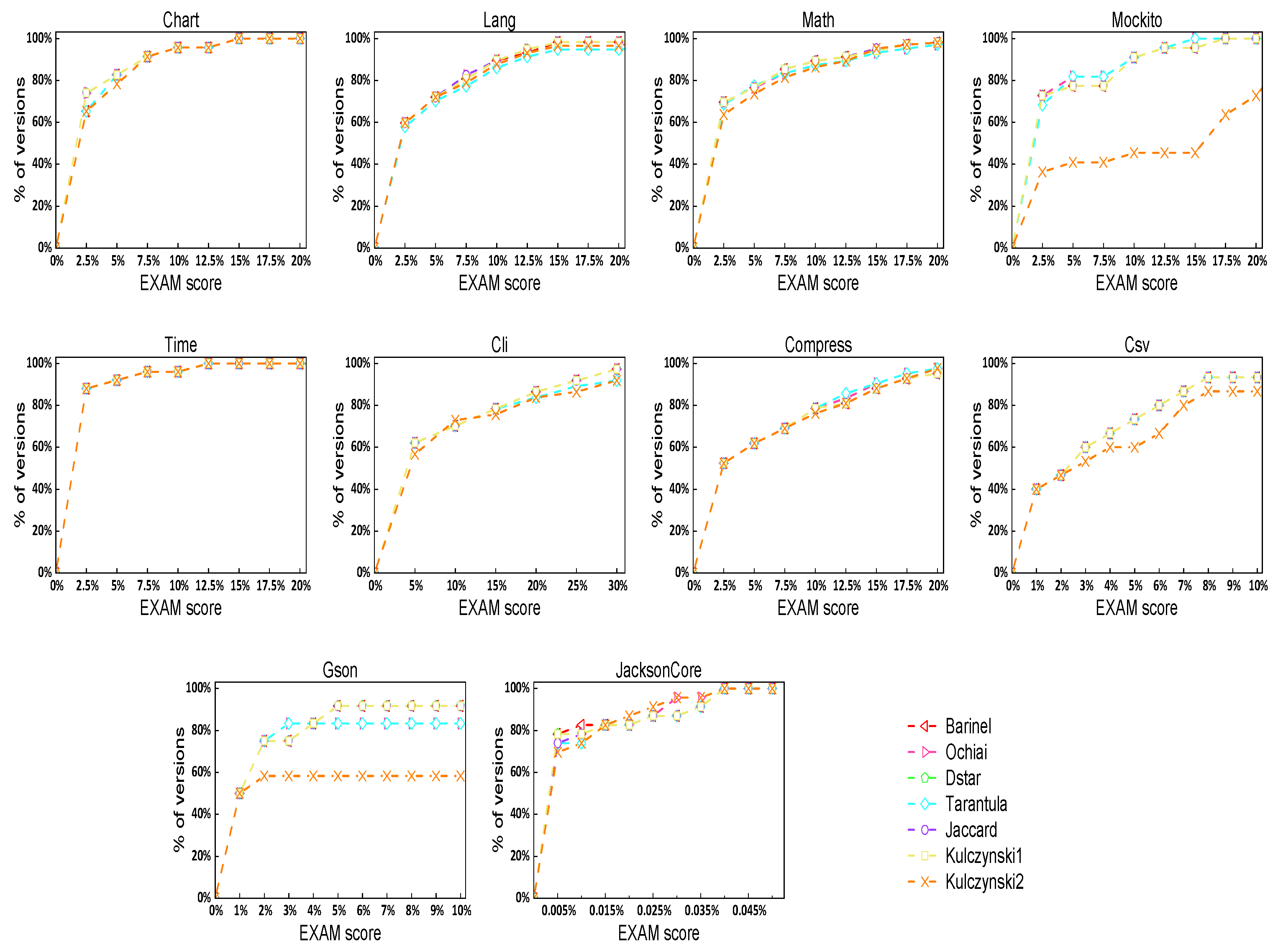
3.4.1. RQ1: What Impact Do Different Suspiciousness Values as Node Weights of the FL-WARMCN Model Have on Fault Location Performance?

We first analyze the fault location performance of the FLWARM-CN model under different suspiciousness algorithms to determine the most suitable indicators for it. We conducted experimental verification using Barinel, Ochiai, Dstar, Tarantula, Jaccard, Kulczynski1, and Kulczynski2 on 10 datasets of defects4J: Lang, Chart, Math, Mockito, Time, Cli, Compress, Csv, Gson, and JacksonCore. The experimental results of ACC@n (TOP-n), EXAM score, and MWE are shown in

Table 2. TOP-1, TOP-3, TOP-5, EXAM, and MWE of FLWARMCN on different datasets.

Subject	FL-WARMCN	Top-1	Top-3	Top-5	EXAM	MWE	Subject	FL-WARMCN	Top-1	Top-3	Top-5	EXAM	MWE
Lang	Barinel	27	34	38	0.0378	14.54	Cli	Barinel	15	19	22	0.0825	48.26
	Ochiai	27	34	38	0.0375	14.52		Ochiai	15	19	22	0.0816	47.61
	Dstar	27	34	38	0.0378	14.54		Dstar	15	19	22	0.0825	48.26
	Tarantula	27	34	38	0.0542	26.89		Tarantula	14	19	23	0.0964	57.74
	Jaccard	27	34	38	0.0375	14.52		Jaccard	15	19	22	0.0825	48.26
	Kulczynski1	27	34	38	0.0378	14.54		Kulczynski1	15	19	22	0.0825	48.26
	Kulczynski2	27	34	38	0.0402	15.54		Kulczynski2	15	20	22	0.0958	54.70
Chart	Barinel	10	12	15	0.0255	74.59	Csv	Barinel	5	7	8	0.0492	16.33
	Ochiai	10	12	15	0.0232	29.76		Ochiai	5	7	8	0.0492	16.33
	Dstar	10	12	15	0.0235	29.63		Dstar	5	7	8	0.0492	16.33
	Tarantula	11	12	15	0.0250	74.15		Tarantula	5	7	8	0.0489	16.20
	Jaccard	10	12	15	0.0235	30.24		Jaccard	5	7	8	0.0492	16.33
	Kulczynski1	10	12	15	0.0235	30.24		Kulczynski1	5	7	8	0.0492	16.33
	Kulczynski2	10	12	13	0.0276	31.20		Kulczynski2	5	7	8	0.0505	16.33
Math	Barinel	44	52	55	0.0336	54.33	Compress	Barinel	14	14	19	0.0606	78.80
	Ochiai	45	54	56	0.0367	55.26		Ochiai	15	15	19	0.0583	78.82
	Dstar	44	52	55	0.0336	54.33		Dstar	14	14	19	0.0607	78.85
	Tarantula	43	54	57	0.0392	64.12		Tarantula	15	15	19	0.0576	78.61
	Jaccard	44	53	56	0.0332	54.25		Jaccard	14	14	19	0.0608	78.87
	Kulczynski1	44	52	55	0.0336	54.33		Kulczynski1	14	14	19	0.0607	78.85
	Kulczynski2	47	56	58	0.0390	72.02		Kulczynski2	15	15	19	0.0610	80.39
Mockito	Barinel	7	10	12	0.0308	42.41	Gson	Barinel	5	7	7	0.0557	140.50
	Ochiai	7	10	12	0.0276	38.45		Ochiai	4	6	6	0.0783	140.00
	Dstar	7	10	12	0.0308	42.41		Dstar	5	7	7	0.0557	140.50
	Tarantula	6	8	10	0.0296	45.18		Tarantula	4	6	6	0.0779	139.33
	Jaccard	7	10	12	0.0308	42.41		Jaccard	5	7	7	0.0557	140.50
	Kulczynski1	7	10	12	0.0308	42.41		Kulczynski1	5	7	7	0.0557	140.50
	Kulczynski2	5	7	7	0.1173	181.11		Kulczynski2	4	6	6	0.1051	198.58
Time	Barinel	4	9	15	0.0130	74.26	JacksonCore	Barinel	9	11	14	0.0072	28.20
	Ochiai	4	9	15	0.0130	74.30		Ochiai	9	12	14	0.0067	28.83
	Dstar	4	9	15	0.0130	74.26		Dstar	8	10	13	0.0072	28.26
	Tarantula	4	9	15	0.0130	73.86		Tarantula	9	11	14	0.0075	31.20
	Jaccard	4	9	15	0.0130	74.26		Jaccard	8	10	14	0.0072	28.87
	Kulczynski1	4	9	15	0.0130	74.26		Kulczynski1	8	10	14	0.0072	28.13
	Kulczynski2	4	9	15	0.0131	74.92		Kulczynski2	10	11	13	0.0071	33.04

. In terms of TOP-1, TOP-3, and TOP-5, Tarantula and Kulczynski2 perform poorly compared to other suspiciousness, especially in the Mockito and Gson projects, while Ochiai, Barinel, Jaccard, and Kulczynski1 perform better on the FLWARM-CN model. In terms of EXAM, as the main indicator of the experiment, Jaccard has the best mean EXAM on all projects; meanwhile, Ochiai has the best performance on Chart, Mockito, JacksonCore, and Cli projects but lags significantly behind Jaccard on Math and Gson. In terms of MWE, Tarantula and Kulczynski2 have significant differences in performance compared to other suspected projects, with Tarantula performing the worst on Lang, Chart, and Cli projects, and Kulczynski2 performing the worst on Math, Mockito, Compress, Gson, and JacksonCore projects. Ochiai, Dstar, Jaccard, and Kulczynski1 have overall better performance on MWE.

To further analyze the distribution of EXAM scores of Barinel, Ochiai, Dstar, Tarantula, Jaccard, Kulczynski1, and Kulczynski2 on different datasets, we show the relationship between EXAM scores and the proportion of faulty versions through line charts, as shown in Figure 2. In Figure 2, the abscissa displays the value of the EXAM score, and the ordinate shows the proportion of the dataset version. Kulczynski2 significantly lags behind other suspiciousness on the Mockito, Csv, and Gson datasets. Tarantula performs better on the Compress and Mockito datasets but performs poorly on the Gson and Cli datasets.

We draw box plots to more comprehensively visualize the performance of Barinel, Ochiai, Dstar, Tarantula, Jaccard, Kulczynski1, and Kulczynski2 in terms of EXAM scores and MWE of the FL-WARMCN model, as shown in Figure 3. The abscissa of Figure 3 represents different suspiciousness, and the ordinate shows the EXAM score and the value of MWE. Different colors mark the box plots corresponding to different suspiciousness. The rectangle represents the box, the upper boundary of the box represents the upper quartile value, and the ratio of the lower boundary of the box represents the lower quartile value. The black horizontal line shows the median and the red horizontal line shows the mean. From Figure 3, we can significantly find that in terms of median, Jaccard and Kulczynski1 have the best performance in MWE and EXAM scores. In terms of the average EXAM score, Jaccard has the best performance, with an average of 0.0398 across 10 datasets. To sum up, we choose Jaccard as the indicator of node weight in the FL-WARMCN model.

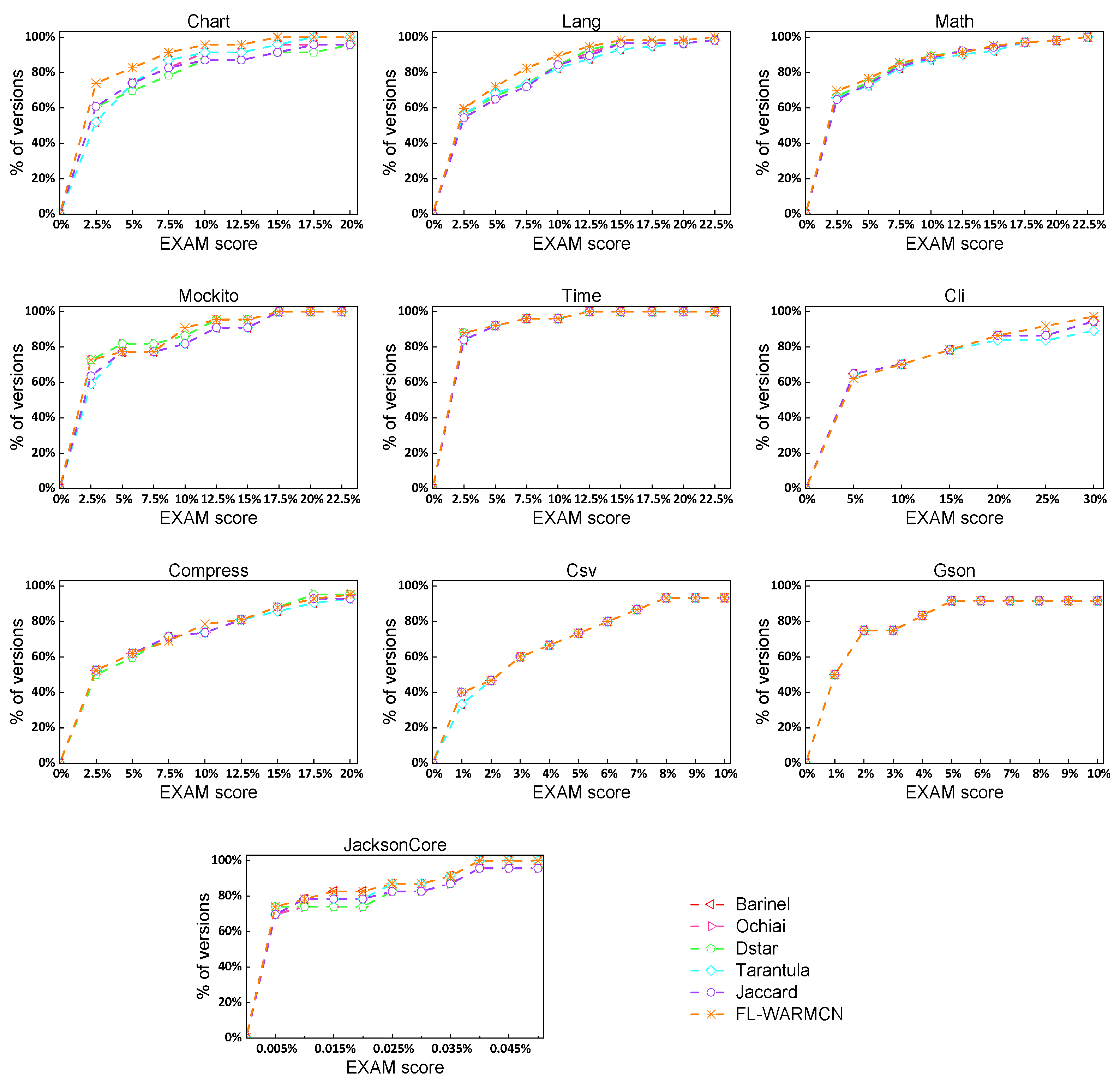
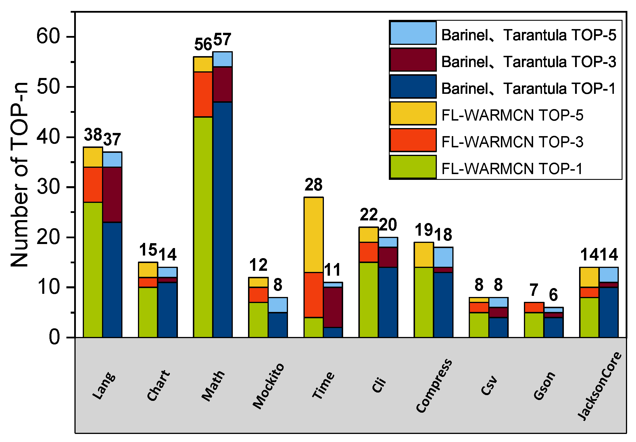
3.4.2. RQ2: Is the FL-WARMCN Model Better Than Other Baseline Fault Location Methods?

After determining the suspiciousness that is most suitable for FL-WARMCN, to evaluate the superiority of the FL-WARMCN model, we selected five commonly used fault location methods: Barinel, Ochiai, Dstar, Tarantula, and Jaccard as baselines. The experimental results of FL-WARMCN and the above five baseline fault location methods in terms of EXAM scores, TOP-1, TOP-3, TOP-5, and MWE on Lang, Chart, Math, Mockito, Time, Cli, Compress, Csv, Gson, and JacksonCore datasets are shown in

Table 3. Comparison of FL-WARMCN and origin Barinel, Ochiai, Dstar, Tarantula, and Jaccard methods in terms of TOP-1, TOP-3, TOP-5, EXAM, and MWE on 10 datasets.

	Barinel	Ochiai	Dstar	Tarantula	Jaccard	FL-WARMCN
EXAM	0.0454	0.0434	0.0436	0.0469	0.0447	0.0398
TOP-1	132	130	131	132	129	139
TOP-3	169	167	168	169	166	175
TOP-5	192	193	193	192	191	206
MWE	59.97	61.66	61.49	61.21	63.79	48.99
Improvement
EXAM	12.33%	8.29%	8.72%	15.14%	10.96%	-
TOP-1	5.30%	6.92%	6.11%	5.30%	7.75%	-
TOP-3	3.55%	4.79%	4.17%	3.55%	5.42%	-
TOP-5	7.29%	6.74%	6.74%	7.29%	7.85%	-
MWE	18.31%	20.55%	20.33%	19.96%	23.20%	-

. FL-WARMCN is 8.29% better than the optimal baseline in EXAM score and is 5.30%, 3.55%, and 6.74% higher than the best fault location method in TOP-1, TOP-3, and TOP-5, respectively. In addition, FL-WARMCN improves MWE by at least 18.31% compared to the baseline fault location method. EXAM represents the ratio between the number of statements before the ranking of faulty statements and the total number of statements, while FL-WARMCN being higher than other baselines means that software debuggers can detect faults by checking fewer statements. For MWE, it quantifies the number of statements before the fault statement ranking and the number of statements with the same ranking as the fault statement. Compared to EXAM, which only focuses on fault localization performance, MWE also considers whether the elements tie in the model localization results is severe. We can find that FL-WARMCN has a more significant performance improvement in MWE compared with other baselines than EXAM, which also indicates that introducing both test case importance and statement importance can effectively break the elements tie.

The experimental results of FL-WARMCN and baseline fault location methods on EXAM scores are shown in Figure 4. We can find that FL-WARMCN is significantly better than other methods on Lang, Chart, Math, Mockito, Cli, and JacksonCore datasets.

To deeply analyze the performance differences between FL-WARMCN and baseline fault location methods on TOP-1, TOP-3, and TOP-5, we selected the two best suspiciousness in terms of TOP-1, TOP-3, and TOP-5 indicators: Barinel and Tarantula. The results of these two suspiciousness algorithms are completely consistent on the Lang, Chart, Math, Mockito, Time, Cli, Compress, Csv, Gson, and JacksonCore datasets. The comparison of the experimental results is shown in Figure 5. The abscissa represents different datasets, the ordinate shows the value of TOP-n, and different colors represent different types of TOP-n values. We can find that compared with the optimal baseline method, the performance of the FL-WARMCN model is significantly improved on the Time and Mockito datasets, improving by 154.55% and 50%, respectively. In addition, the application of the FL-WARMCN model on Lang, Time, Mockito, Cli, Comparess, Csv, and Gson datasets can enable software debuggers to determine the accurate location of faults faster.

To further analyze the performance differences between the FL-WARMCN model and other baseline methods, we used the Wilcoxon signed-rank test [49]. The Wilcoxon signed-rank test is a non-parametric pairing test method that does not require any assumptions about the distribution of samples. This method has been widely used in SBFL research [20,43,47,48,50]. The null hypothesis ($H_0$) indicates that there is no significant difference between the two baselines, and a p-value less than 0.05 indicates a significant difference between the two baselines. The experimental results of the FL-WARMCN model and other baseline Wilcoxon signed rank tests are shown in

Table 4. Comparison of Wilcoxon signed-rank test results between FL-WARMCN, Barinel, Ochiai, Dstar, Tarantula, and Jaccard.

${\mathit{H}}_0$	p-Value
FL-WARMCN = Barinel	$5.87\times {10}^{-8}$
FL-WARMCN = Ochiai	$3.98\times {10}^{-3}$
FL-WARMCN = Dstar	$3.49\times {10}^{-2}$
FL-WARMCN = Tarantula	$2.19\times {10}^{-8}$
FL-WARMCN = Jaccard	$2.03\times {10}^{-5}$

. The experimental results show that FL-WARMCN is significantly better than Barinel, Ochiai, Dstar, Tarantula, and Jaccard in terms of EXAM (p-values are all less than 0.05).

In summary, the above experiments indicate that the FL-WARMCN model can effectively break the elements tie by simultaneously considering the importance of test cases and statements. Assigning weights to test cases and utilizing the centrality of feature vectors to calculate statement importance can effectively redirect suspicion calculation to more important fault statements and test cases, thereby improving software fault localization performance.

4. Discussion

4.1. How Much Improvement Has Been Made in the Fault Localization Efficiency of the FL-WARMCN Model?

In this section, we comprehensively analyze the improvement of the FL-WARMCN model in fault location capabilities through quantity and accuracy. TOP-1, TOP-3, and TOP-5 are applied to quantify the improvement of the FL-WARMCN model in the number of located faults; EXAM and MWE describe the accuracy of fault location tasks.

In the experiment in Section 3.4.2, we compared Jaccard as the node weight with the classic method to more directly evaluate the improvement of fault location efficiency of the FL-WARMCN model. We apply the Barinel, Ochiai, Dstar, Tarantula, and Jaccard methods, respectively, to compare with the FL-WARMCN model as node weights in terms of TOP-n, EXAM score, and MWE, as shown in Figure 6. In terms of TOP-1, TOP-3, and TOP-5, Ochiai and Jaccard have improved significantly, both exceeding 5%. The overall FL-WARMCN model is more obvious in TOP-1 and TOP-5. Barinel, Dstar, and Tarantula are slightly less effective in improving TOP-3 than the other two indicators. In terms of EXAM scores, Tarantula has a limited improvement effect, while Barinel and Jaccard’s methods both improve by more than 10%. As for the MWE value, FL-WARMCN has improved by more than 20% in the Ochiai, Dstar, and Jaccard indicators, and the fault location effect has been significantly improved. From the above results, it is not difficult to find that the FL-WARMCN model has a significant improvement effect on these five classic fault location methods.

4.2. What Is the Impact of Different EDGE weights on the Localization Performance of FL-WARMCN?

In Section 3.4.1, we determined the most suitable node weight method for the FL-WARMCN model. However, in the network structure constructed by FLWARMCN, edge weights measure the correlation between statements. Different correlation measurement methods directly affect the eigenvector centrality of statements, leading to different ranking results of faulty statements. Therefore, whether Accuracy is the optimal edge weight in the network is still a debatable issue. We have chosen two commonly used correlation indicators in ARM algorithms, Lift [51] and Support [52]. The EXAM scores of the FL-WARMCN model using Accuracy, Lift, and Support as edge weights on 10 datasets are shown in

Table 5. The EXAM score of FL-WARMCN model using Accuracy, Lift, and Support as edge weights on 10 datasets.

Datasets	Accuracy	Lift	Support
Chart	0.0251	0.0256	0.0754
Lang	0.0375	0.0376	0.0500
Math	0.0332	0.0346	0.0650
Mockito	0.0308	0.0316	0.0604
Time	0.0130	0.0132	0.0627
Cli	0.0825	0.0844	0.1296
Compress	0.0608	0.0622	0.0991
Csv	0.0492	0.0489	0.1160
Gson	0.0557	0.0542	0.0942
JacksonCore	0.0072	0.0073	0.0073
W/T/L	-	8/0/2	10/0/0

. The Win/Tie/Loss relationship of Accuracy compared to Lift on 10 datasets is 8/0/2, with Accuracy only having lower EXAM on Csv and Gson datasets compared to Lift, while outperforming Lift on the remaining eight datasets. Accuracy is significantly better than the Support on all 10 datasets. Therefore, accuracy is the most suitable edge weight for the FL-WARMCN model in terms of EXAM.

In terms of TOP-n, the FL-WARMCN model uses accuracy, lift, and support as edge weights for TOP-1, Top-3, and TOP-5, as shown in Figure 7. Accuracy outperforms the other two edge weights in TOP-1 on the Math dataset and is consistent with Lift on the Mockito, Time, Cli, Compress, Csv, Gson, and JacksonCore datasets, all of which are superior to Support. In terms of TOP-3, Accuracy is the best edge weight on the Math, Lang, Cli, and Compress datasets, while its performance is on par with Lift on datasets other than Time. For TOP-5, Accuracy is the best edge weight on the Math, Lang, and Chart datasets and only slightly inferior to Lift on the Mockito dataset. Therefore, in the TOP-n metric, Accuracy performs better than Lift while Support performs the worst as the edge weight performance of the FL-WARMCN model.

4.3. What Is the Computational Complexity of the FL-WARMCN Model?

To determine whether the computational complexity of the FL-WARMCN model is acceptable, we compared it with the computational complexity of the SBFL method based on complex network theory (FLCN) [19]. The computational complexity is mainly divided into time complexity and space complexity. The time complexity quantifies the time consumed by the model to run, assuming that there are M statements and N test cases in the tested program. The FLCN model constructs a network by calculating the correlation between pairwise statements. This process requires first traversing N test cases and then traversing M statements, repeating the process twice. Therefore, the time complexity of this process is $O(2\ast N\ast M)$. After constructing the network, the FLCN model traverses each node to calculate its degree centrality, with a time complexity of $O\left(M\right)$. As mentioned above, the time complexity of the FLCN model is $O(N\ast M)$. The FL-WARMCN model first calculates the time complexity of test case weights as $O\left(N\right)$ and then uses the suspiciousness to calculate node weights; so, the time complexity of this process is $O(M\ast N)$. After obtaining the node weights, the time complexity of the FL-WARMCN model in constructing the network is the same as FLCN, which is also $O(2\ast N\ast M)$. The time complexity of calculating the weighted suspiciousness of statements through the eigenvector centrality is $O\left(M\right)$. Therefore, the total time complexity of the FL-WARMCN model is $O(N\ast M)$.

The space complexity measures the storage space occupied by the model during operation, assuming that there are M statements and N test cases in the tested program. The FLCN model constructs a network by storing the correlation between statements and stores the degree centrality of each statement when calculating suspiciousness of statements; therefore, its space complexity is $O\left(M^2\right)$. Similarly, the FL-WARMCN model first stores the space complexity $O\left(N\right)$ used for the weights of test cases, while the space complexity $O\left(M\right)$ is used for calculating node weights, and the space complexity $O\left(M^2\right)$ is used for storing the relationship between pairwise statements in calculating edge weights. Considering that the number of M is often significantly greater than N, the overall space complexity of the FL-WARMCN model is $O\left(M^2\right)$. In summary, although the FL-WARMCN model has increased the calculation of node weights and test case weights compared to the FLCN model [19], FL-WARMCN and FLCN still maintain consistency in terms of time complexity and space complexity.

5. Threats to Validity

5.1. Internal Validity

Our proposed FL-WARMCN model is implemented in Python 3.9 and utilizes the pandas, numpy, and networkx libraries, which are well-established and reliable in the research field. Additionally, our experimental subjects were sourced from the Defects4J dataset, which has been proven to be reliable in a large number of existing SBFL studies [2,7,9,12,24,25,26,47,48]. We have thoroughly reviewed all the experiment’s code to ensure its accuracy.

5.2. External Validity

We selected 10 open-source Java projects from the Defects4J dataset as experimental subjects to fully evaluate the effectiveness and superiority of the FL-WARMCN model. The number of experimental subjects is sufficient and appropriate for model evaluation. However, the use of Java as the development language in the selected projects may limit the effective application of the FL-WARMCN model to projects in other programming languages. On the other hand, all algorithms compared in the experiment use the same program spectrum as input to ensure a fair evaluation of the differences in fault location performance. The evaluation metrics Exam, acc@n, and MWE, which were adopted for the experiment, have also been widely used in SBFL research.

6. Conclusions

In this paper, we propose the FL-WARMCN model to enhance fault location performance. The model utilizes Jaccard to assign different weights to each test case, quantifying their importance. On this basis, we introduce statement importance and establish association relationships between numerous statements and their suspiciousness using weighted association rule mining technology. These association relationships are applied to construct the edges and edge weights of complex networks, and the statements and their suspiciousness serve as nodes and node weights, respectively. FL-WARMCN employs eigenvector centrality as the criterion for determining the importance of statements, taking into account both the node’s degree and the importance of its neighboring nodes. Finally, we calculate the final suspiciousness of each statement by multiplying its statement importance and statement suspiciousness, arranging them in descending order to obtain the fault location result. We conducted four comprehensive experiments to evaluate the superiority of FL-WARMCN. The results indicate that Jaccard is the most suitable node weight for the FL-WARMCN model and that FL-WARMCN outperforms other baseline methods significantly. Furthermore, we conducted a further analysis of the impact of different edge weights on the model’s performance.

Although the FL-WARMCN model effectively breaks the elements tie, it still has some limitations. The input of the model only comes from statement coverage information, and the semantic information in the program source code has not been fully considered. In future work, we expect to add more code semantic information to the FL-WARMCN model through natural language processing (NLP) techniques to analyze the importance of statements more deeply and effectively.

References

1. Sohn, J.; Yoo, S. Empirical evaluation of fault localisation using code and change metrics. IEEE Trans. Softw. Eng. 2019, 47, 1605–1625. [Google Scholar] [CrossRef]
2. Sarhan, Q.I.; Beszédes, Á. A survey of challenges in spectrum-based software fault localization. IEEE Access 2022, 10, 10618–10639. [Google Scholar] [CrossRef]
3. Abreu, R.; Zoeteweij, P.; Van Gemund, A.J. Spectrum-based multiple fault localization. In Proceedings of the 2009 IEEE/ACM International Conference on Automated Software Engineering, Auckland, New Zealand, 16–20 November 2009; pp. 88–99. [Google Scholar]
4. Abreu, R.; Zoeteweij, P.; Van Gemund, A.J. On the accuracy of spectrum-based fault localization. In Proceedings of the Testing: Academic and Industrial Conference Practice and Research Techniques-MUTATION (TAICPART-MUTATION 2007), Windsor, UK, 10–14 September 2007; pp. 89–98. [Google Scholar]
5. Wong, W.E.; Debroy, V.; Choi, B. A family of code coverage-based heuristics for effective fault localization. J. Syst. Softw. 2010, 83, 188–208. [Google Scholar] [CrossRef]
6. Jones, J.A.; Harrold, M.J.; Stasko, J. Visualization of test information to assist fault localization. In Proceedings of the 24th International Conference on Software Engineering, Orlando, FL, USA, 25 May 2002; pp. 467–477. [Google Scholar]
7. Golagha, M.; Pretschner, A. Challenges of operationalizing spectrum-based fault localization from a data-centric perspective. In Proceedings of the 2017 IEEE International Conference on Software Testing, Verification and Validation Workshops (ICSTW), Tokyo, Japan, 13–17 May 2017; pp. 379–381. [Google Scholar]
8. Wong, W.E.; Gao, R.; Li, Y.; Abreu, R.; Wotawa, F. A survey on software fault localization. IEEE Trans. Softw. Eng. 2016, 42, 707–740. [Google Scholar] [CrossRef]
9. Wang, T.; Yu, H.; Wang, K.; Su, X. Fault localization based on wide & deep learning model by mining software behavior. Future Gener. Comput. Syst. 2022, 127, 309–319. [Google Scholar]
10. Liu, H.; Li, Z.; Wang, H.; Liu, Y.; Chen, X. CRMF: A fault localization approach based on class reduction and method call frequency. Softw. Pract. Exp. 2023, 53, 1061–1090. [Google Scholar] [CrossRef]
11. Youm, K.C.; Ahn, J.; Lee, E. Improved bug localization based on code change histories and bug reports. Inf. Softw. Technol. 2017, 82, 177–192. [Google Scholar] [CrossRef]
12. Peng, Z.; Xiao, X.; Hu, G.; Sangaiah, A.K.; Atiquzzaman, M.; Xia, S. ABFL: An autoencoder based practical approach for software fault localization. Inf. Sci. 2020, 510, 108–121. [Google Scholar] [CrossRef]
13. Li, X.; Li, W.; Zhang, Y.; Zhang, L. Deepfl: Integrating multiple fault diagnosis dimensions for deep fault localization. In Proceedings of the 28th ACM SIGSOFT International Symposium on Software Testing and Analysis, Beijing, China, 15–19 July 2019; pp. 169–180. [Google Scholar]
14. Wong, W.E.; Debroy, V.; Golden, R.; Xu, X.; Thuraisingham, B. Effective software fault localization using an RBF neural network. IEEE Trans. Reliab. 2011, 61, 149–169. [Google Scholar] [CrossRef]
15. Xiao, X.; Pan, Y.; Zhang, B.; Hu, G.; Li, Q.; Lu, R. ALBFL: A novel neural ranking model for software fault localization via combining static and dynamic features. Inf. Softw. Technol. 2021, 139, 106653. [Google Scholar] [CrossRef]
16. Qian, J.; Ju, X.; Chen, X. GNet4FL: Effective fault localization via graph convolutional neural network. Autom. Softw. Eng. 2023, 30, 16. [Google Scholar] [CrossRef]
17. Dorogovtsev, S.N.; Mendes, J.F. Evolution of Networks: From Biological Nets to the Internet and WWW; Oxford University Press: Oxford, UK, 2003. [Google Scholar]
18. Prignano, L.; Moreno, Y.; Díaz-Guilera, A. Exploring complex networks by means of adaptive walkers. Phys. Rev. E 2012, 86, 066116. [Google Scholar] [CrossRef] [PubMed]
19. Zakari, A.; Lee, S.P.; Chong, C.Y. Simultaneous localization of software faults based on complex network theory. IEEE Access 2018, 6, 23990–24002. [Google Scholar] [CrossRef]
20. Zakari, A.; Lee, S.P.; Hashem, I.A.T. A single fault localization technique based on failed test input. Array 2019, 3, 100008. [Google Scholar] [CrossRef]
21. Zhu, L.Z.; Yin, B.B.; Cai, K.Y. Software fault localization based on centrality measures. In Proceedings of the 2011 IEEE 35th Annual Computer Software and Applications Conference Workshops, Munich, Germany, 18–22 July 2011; pp. 37–42. [Google Scholar]
22. He, H.; Ren, J.; Zhao, G.; He, H. Enhancing spectrum-based fault localization using fault influence propagation. IEEE Access 2020, 8, 18497–18513. [Google Scholar] [CrossRef]
23. Bandyopadhyay, A.; Ghosh, S. Proximity based weighting of test cases to improve spectrum based fault localization. In Proceedings of the 2011 26th IEEE/ACM International Conference on Automated Software Engineering (ASE 2011), Lawrence, KS, USA, 6–10 November 2011; pp. 420–423. [Google Scholar]
24. Yoshioka, H.; Higo, Y.; Kusumoto, S. Improving Weighted-SBFL by Blocking Spectrum. In Proceedings of the 2022 IEEE 22nd International Working Conference on Source Code Analysis and Manipulation (SCAM), Limassol, Cyprus, 3 October 2022; pp. 253–263. [Google Scholar]
25. Yang, X.; Liu, B.; An, D.; Xie, W.; Wu, W. A Fault Localization Method Based on Similarity Weighting with Unlabeled Test Cases. In Proceedings of the 2022 IEEE 22nd International Conference on Software Quality, Reliability, and Security Companion (QRS-C), Guangzhou, China, 5–9 December 2022; pp. 368–374. [Google Scholar]
26. Zhang, M.; Li, Y.; Li, X.; Chen, L.; Zhang, Y.; Zhang, L.; Khurshid, S. An empirical study of boosting spectrum-based fault localization via pagerank. IEEE Trans. Softw. Eng. 2019, 47, 1089–1113. [Google Scholar] [CrossRef]
27. Yi, Z.; Wei, L.; Wang, L. Research on association rules based on Complex Networks. In Proceedings of the 2016 2nd Workshop on Advanced Research and Technology in Industry Applications (WARTIA-16), Dalian, China, 14–15 May 2016; pp. 1627–1632. [Google Scholar]
28. Choobdar, S.; Silva, F.; Ribeiro, P. Network node label acquisition and tracking. In Proceedings of the Progress in Artificial Intelligence: 15th Portuguese Conference on Artificial Intelligence (EPIA 2011), Lisbon, Portugal, 10–13 October 2011; pp. 418–430. [Google Scholar]
29. Zhang, H.; Wang, M.; Deng, W.; Zhou, J.; Liu, L.; Li, J.; Li, R. Identification of Key Factors and Mining of Association Relations in Complex Product Assembly Process. Int. J. Aerosp. Eng. 2022, 2022, 2583437. [Google Scholar] [CrossRef]
30. Zhou, Y.; Li, C.; Ding, L.; Sekula, P.; Love, P.E.; Zhou, C. Combining association rules mining with complex networks to monitor coupled risks. Reliab. Eng. Syst. Saf. 2019, 186, 194–208. [Google Scholar] [CrossRef]
31. Agrawal, R.; Srikant, R. Fast algorithms for mining association rules. In Proceedings of the 20th International Conference on Very Large Data Bases, Santiago, Chile, 12–15 September 1994; Volume 1215, pp. 487–499. [Google Scholar]
32. Baralis, E.; Cagliero, L.; Cerquitelli, T.; Chiusano, S.; Garza, P. Digging deep into weighted patient data through multiple-level patterns. Inf. Sci. 2015, 322, 51–71. [Google Scholar] [CrossRef]
33. Sun, K.; Bai, F. Mining weighted association rules without preassigned weights. IEEE Trans. Knowl. Data Eng. 2008, 20, 489–495. [Google Scholar] [CrossRef]
34. Kleinberg, J.M. Authoritative sources in a hyperlinked environment. J. ACM (JACM) 1999, 46, 604–632. [Google Scholar] [CrossRef]
35. Weng, C.H.; Huang, T.C.K. Knowledge acquisition of association rules from the customer-lifetime-value perspective. Kybernetes 2018, 47, 441–457. [Google Scholar] [CrossRef]
36. Zhang, M.; Wang, S.; Wu, W.; Qiu, W.; Xie, W. A Software Multi-Fault Clustering Ensemble Technology. In Proceedings of the 2022 IEEE 22nd International Conference on Software Quality, Reliability, and Security Companion (QRS-C), Guangzhou, China, 5–9 December 2022; pp. 352–358. [Google Scholar]
37. Shao, Y.; Liu, B.; Wang, S.; Li, G. A novel software defect prediction based on atomic class-association rule mining. Expert Syst. Appl. 2018, 114, 237–254. [Google Scholar] [CrossRef]
38. He, Z.; Huang, D.; Fang, J. Social stability risk diffusion of large complex engineering projects based on an improved SIR model: A simulation research on complex networks. Complexity 2021, 2021, 7998655. [Google Scholar] [CrossRef]
39. Adeleye, O.; Yu, J.; Wang, G.; Yongchareon, S. Constructing and evaluating evolving web-API Networks-A complex network perspective. IEEE Trans. Serv. Comput. 2021, 16, 177–190. [Google Scholar] [CrossRef]
40. Mheich, A.; Wendling, F.; Hassan, M. Brain network similarity: Methods and applications. Netw. Neurosci. 2020, 4, 507–527. [Google Scholar] [CrossRef]
41. Wandelt, S.; Shi, X.; Sun, X. Estimation and improvement of transportation network robustness by exploiting communities. Reliab. Eng. Syst. Saf. 2021, 206, 107307. [Google Scholar] [CrossRef]
42. Pearson, S.; Campos, J.; Just, R.; Fraser, G.; Abreu, R.; Ernst, M.D.; Pang, D.; Keller, B. Evaluating and improving fault localization. In Proceedings of the 2017 IEEE/ACM 39th International Conference on Software Engineering (ICSE), Buenos Aires, Argentina, 20–28 May 2017; pp. 609–620. [Google Scholar]
43. Wong, W.E.; Debroy, V.; Gao, R.; Li, Y. The DStar method for effective software fault localization. IEEE Trans. Reliab. 2013, 63, 290–308. [Google Scholar] [CrossRef]
44. Wolfe, A.W. Social network analysis: Methods and applications. Am. Ethnol. 1997, 24, 219–220. [Google Scholar] [CrossRef]
45. Tudisco, F.; Arrigo, F.; Gautier, A. Node and layer eigenvector centralities for multiplex networks. SIAM J. Appl. Math. 2018, 78, 853–876. [Google Scholar] [CrossRef]
46. Just, R.; Jalali, D.; Ernst, M.D. Defects4J: A database of existing faults to enable controlled testing studies for Java programs. In Proceedings of the 2014 International Symposium on Software Testing and Analysis, San Jose, CA, USA, 21–25 July 2014; pp. 437–440. [Google Scholar]
47. Yan, X.; Liu, B.; Wang, S. A Test Restoration Method based on Genetic Algorithm for effective fault localization in multiple-fault programs. J. Syst. Softw. 2021, 172, 110861. [Google Scholar] [CrossRef]
48. Lei, Y.; Xie, H.; Zhang, T.; Yan, M.; Xu, Z.; Sun, C. Feature-fl: Feature-based fault localization. IEEE Trans. Reliab. 2022, 71, 264–283. [Google Scholar] [CrossRef]
49. Demšar, J. Statistical comparisons of classifiers over multiple data sets. J. Mach. Learn. Res. 2006, 7, 1–30. [Google Scholar]
50. Gao, R.; Wong, W.E.; Chen, Z.; Wang, Y. Effective software fault localization using predicted execution results. Softw. Qual. J. 2017, 25, 131–169. [Google Scholar] [CrossRef]
51. Besharati, M.M.; Tavakoli Kashani, A. Which set of factors contribute to increase the likelihood of pedestrian fatality in road crashes? Int. J. Inj. Control Saf. Promot. 2018, 25, 247–256. [Google Scholar] [CrossRef] [PubMed]
52. Wu, W.; Wang, S.; Liu, B.; Shao, Y.; Xie, W. A novel software defect prediction approach via weighted classification based on association rule mining. Eng. Appl. Artif. Intell. 2024, 129, 107622. [Google Scholar] [CrossRef]
Figure 1. The FL-WARMCN model framework.
Mathematics 12 02113 g001
Figure 2. Experimental comparison results of EXAM scores using Barinel, Ochiai, Dstar, Tarantula, Jaccard, Kulczynski1, and Kulczynski2 as suspiciousness in FL-WARMCN on 10 datasets.
Mathematics 12 02113 g002
Figure 3. Experimental comparison results of MWE and EXAM scores using Barinel, Ochiai, Dstar, Tarantula, Jaccard, Kulczynski1, and Kulczynski2 as suspiciousness in FL-WARMCN.
Mathematics 12 02113 g003
Figure 4. Experimental comparison results of FL-WARMCN and Barinel, Ochiai, Dstar, Tarantula, and Jaccard algorithms in terms of EXAM scores on 10 datasets.
Mathematics 12 02113 g004
Figure 5. Experimental comparison results of TOP-1, TOP-3, and TOP-5 between FL-WARMCN and the best baseline algorithm on Lang, Chart, Math, Mockito, Time, Cli, Compress, Csv, Gson, and JacksonCore datasets.
Mathematics 12 02113 g005
Figure 6. Experimental comparison results of improvements in TOP-n, EXAM, and MWE of Barinel, Ochiai, Dstar, Tarantula, and Jaccard methods after applying FL-WARMCN model.
Mathematics 12 02113 g006
Figure 7. The TOP-n of FL-WARMCN model using Accuracy, Lift, and Support as edge weights on 10 datasets.
Mathematics 12 02113 g007