Optimal Investment for Defined-Contribution Pension Plans with the Return of Premium Clause under Partial Information

Abstract

The optimal investment problem for defined contribution (DC) pension plans with partial information is the subject of this paper. The purpose of the return of premium clauses is to safeguard the rights of DC pension plan participants who pass away during accumulation. We assume that the market price of risk consists of observable and unobservable factors that follow the Ornstein-Uhlenbeck processes, and the pension fund managers estimate the unobservable component from known information through Bayesian learning. Considering maximizing the expected utility of fund wealth at the terminal time, optimal investment strategies and the corresponding value function are determined using the dynamical programming principle approach and the filtering technique. Additionally, fund managers forsake learning, which results in the presentation of suboptimal strategies and utility losses for comparative analysis. Lastly, numerical analyses are included to demonstrate the impact of model parameters on the optimal strategy.

1. Introduction

With the increasingly severe issue of an aging population, the scale of the contributing demographic is decreasing, while the demographic receiving pension benefits is on the rise. The pay-as-you-go pension system carries a substantial implicit liability, facing an unsustainable predicament. In contrast, the defined contribution (DC) pension plan invests contributions in the capital market, achieving the accumulation and appreciation of funds to meet the demands of pension payouts. The DC pension plan can effectively cope with the impact of population aging. Therefore, the study of assets allocation in the DC pension plan has important theoretical and practical value.

The optimal investment strategy in the accumulation phase of the DC plan has been the subject of extensive research in recent years, utilizing a variety of objective functions and financial market structures. On one hand, many attempts have made to study the optimal investment problems under the criterion of mean-variance (see e.g., Li and Ng (2000) [1], Xiao et al. (2020) [2]). On the other hand, scholars studied optimization problems matters with the goal of optimizing the anticipated utility of terminal riches. For instance, in a complete financial market with a stochastic interest rate, Battocchio and Menoncin (2004) [3] optimize the expected utility of his terminal wealth. Han and Hung (2012) [4] examined the scenario of downside protection in the context of stochastic inflation and identified the optimal investment strategy to optimize the expected utility of terminal wealth. A derivative-based optimal investment strategy for a pension investor who is ambiguity-averse and has time-varying income and market return volatility was proposed by Zeng et al. (2018) [5]. Wang et al. (2021a) [6] examined a robust optimal portfolio selection problem for DC pension plan members that are concerned about model ambiguity. For other related work about DC pension management may refer to Wang and Li (2018) [7], Dong and Zheng (2019) [8], Lv et al. (2023) [9] and references therein.

It has been widely recognized that the accumulation phase of DC pension programs is associated with a risk of mortality. To protect the rights of participants who die during the accumulation phase, a return of premium clause is usually attached to traditional DC pension plans, which means that the designated beneficiaries of participants who die before retirement can withdraw the pension accumulated during the participants’ working period. He and Liang (2013) [10] first incorporated the actuarial rules of return of premium clauses into the stochastic control problem under the continuous-time framework. Subsequently, Bian et al. (2018) [11] delved into the exploration of optimal pre-commitment strategies for DC pension funds encompassing return of premium clauses, albeit within the context of discrete-time framework. The robust equilibrium strategy for a mean-variance DC pension plan with ambiguity aversion and premium return clauses was examined by Chang and Li (2023) [12] under the jump-diffusion model. For further inquiries into this subject, interested parties are encouraged to consult the studies by Li et al. (2017) [13], Lai et al. (2021) [14], and the research by Nie et al. (2023) [15].

The aforementioned studies adopted deterministic functions to describe the drift terms (expected return) and diffusion terms (volatility) of the controlled processes. However, the expected return of risky assets is unobservable and difficult to estimate. There is ample evidence from empirical studies that the expected returns of risky assets are predictable (see e.g., Fama and French (1988) [16], Boudoukh et al. (2007) [17]). Brennan (1998) [18] pointed out that even if decision makers do not have exact information about the expected return of risky assets at the time of allocation, they will “learn” the unobservable information as the observable information accumulates. When estimating the expected returns and dividend growth rates of the aggregate stock market, Van Binsbergen and Koijen (2010) [19] presupposed the unobservability of one of the predictive variables. Branger et al. (2013) [20], in their modeling of an ambiguity-aversion investor with constant interest rates and stock return volatility, made the same assumption regarding predictors within a utility maximization framework. Escobar et al. (2016) [21] subsequently postulate that the stock risk premium is an affine function of the predictive variables, with the observed factor determining stock return volatility. Wang et al. (2021b) [22] subsequently examined the equilibrium investment strategies for DC pension funds, proposing that the expected return on the stock is influenced by an unobservable predictor that follows a mean-reverting stochastic process. This topic is thoroughly examined in the works of Xia (2001) [23], Huang and Chen (2021) [24], and Wang et al. (2022) [25]. In contrast to this corpus of research, we address the optimal investment problem for DC pension funds by integrating premium clause return, stochastic volatility, and stock return predictability.

This paper investigates the optimal portfolio strategy for DC pension funds under partial information. Fund managers allocate the wealth of the fund to the financial market, which encompasses both risky and risk-free assets. We suppose that the stock risk premium is driven by both observable and unobservable factors, reflecting that the observable part can not fully explain the variations in the risk premium. Empirical studies (e.g., Harvey (2001) [26], Whitelaw (1994) [27]) have suggested that the expected return and volatilities of risky assets may be driven by the same factors. Consequently, we presume that the observed factor determines the volatility of stock returns, which means that the stochastic volatility model is a specific case in our general model. The objective of the optimization problem is to maximize the expected power utility of the terminal wealth. Applying the Kalman filter theory and solving the Hamilton-Jacobi-Bellman (HJB) equation, we derive semi-analytical form solutions for the optimal portfolios and value function. Additionally, we deduce that the failure to adopt learning results in suboptimal strategies and utility losses. Lastly, the Monte Carlo method is employed to ascertain the optimal investment strategy and the utility losses associated with suboptimal strategies for empirically relevant parameter values. In addition, the numerical analysis illustrates an instance of the stochastic volatility process, which confirms that optimal portfolios with properties that are consistent with well-known stochastic volatility models are generated by general volatility.

We are of the opinion that this paper suggests three substantial innovations when compared to the existing literature: (1) The optimal investment for defined-contribution pension plans with the return of premium clause under partial information is derived, and at the mathematical level, the verification theorem and theoretical results for this model has distinct differences from the literature. (2) The risk premium is characterized by both observed and unobserved factors, while stock volatility is dirven by the observed factor, which is rarely taken into account in the literature. The general volatility model gives more flexibility in fitting the price of risky assets. (3) Our numerical results unequivocally demonstrate the prudence of acknowledging the influence of “prediction” and the significance of rational portfolio for the DC pension fund, thereby revealing the utility losses that result from disregarding learning.

The remainder of this paper is organized as follows: The model and assumptions regarding the financial market are delineated in Section 2. The optimization problem is resolved in Section 3. The numerical illustrations in Section 4 are intended to facilitate the analysis of our findings. The paper is concluded in Section 5.

2. Model and Assumptions

In this section, we consider a continuous-time financial market under the following assumptions. The fund manager has the ability to trade in the financial market without incurring any additional fees or taxes. We consider $(\mathsf{\Omega },\mathcal{F},\mathrm{P})$ to be a full probability space that has a ${\left\{{\mathcal{F}}_t\right\}}_{t\in [0,T]}$ filtration, in which ${\mathcal{F}}_t$ denotes market information until time t. The time horizon is represented by the finite constant $T>0.$ Consider that the probability space is well-defined for all stochastic processes and random variables, and that any decision made at time t is made using ${\mathcal{F}}_t$.

2.1. Financial Market and Filtered Estimation

We presume that the financial market comprises one risk-free asset and one risky asset. The price of the risk-free asset $S_0(t)$ can be determined by employing the following formula:

$$\frac{\mathrm{d}{S}_0(t)}{S_0(t)}=r\mathrm{d}t.$$

(1)

The risk-free interest rate is represented by $r>0.$ $S_1(t)$, being the risky asset’s price, is subject to a geometric Brownian motion:

$$\frac{\mathrm{d}{S}_1(t)}{S_1(t)}={\mu }_s(t)\mathrm{d}t+{\sigma }_s(t)\mathrm{d}{W}_s(t),$$

(2)

where ${\mu }_s(t)$ represents the expected return of the risky asset, and ${\sigma }_s(t)>0$ corresponds to volatility.

$\frac{{\mu }_s(t)-r}{{\sigma }_s(t)}={\delta }_{m}m(t)+{\delta }_{n}n(t)+\delta$ is market price of risk, representing the excess return that bears per unit of increase in risk. $\delta ,{\delta }_m$ and ${\delta }_n$ are real constants. $m(t)$ and $n(t)$ represent the observable and unobservable factors, respectively, which reflects the fact that the observable information cannot perfectly explain the changes in the stock risk premium. ${\delta }_m$ and ${\delta }_n$ represents the predictive power of $m(t)$ and $n(t)$, respectively. Assuming that $m(t)$ and $n(t)$ follow the Ornstein-Uhlenbeck process

$$\begin{array}{cc}\hfill & \mathrm{d}m(t)=k_m[\overline{m}-m(t)]\mathrm{d}t+{\sigma }_m\mathrm{d}{W}_m(t),\hfill \\ \hfill & \mathrm{d}n(t)=k_n[\overline{n}-n(t)]\mathrm{d}t+{\sigma }_n\mathrm{d}{W}_n(t).\hfill \end{array}$$

(3)

$k_m>0$ and $k_n>0$ are liquidity parameters that control the mean-reverting degree of the two random factors $m(t)$ and $n(t)$, while $\overline{m}$ and $\overline{n}$ denote the long-term means of $m(t)$ and $n(t)$, respectively. ${\sigma }_m>0$ and ${\sigma }_n>0$ correspond to the volatilities. $W_s(t)$, $W_m(t)$, and $W_n(t)$ are correlated 1-dimensional standard Brownian motions with correlation coefficients $p_{sm}$, $p_{sn}$, and $p_{nm}$, i.e., $\mathrm{Cov}(W_s(t),W_m(t))=p_{ms}t$, $\mathrm{Cov}(W_s(t),W_n(t))=p_{ns}t$, $\mathrm{Cov}(W_m(t)W_n(t))=p_{nm}t$. We further postulate that the observed factor, i.e., ${\sigma }_s(t)={\sigma }_s(m(t))$, influences stock return volatility, which is consistent with the empirical findings of Harvey (2001) [26], Whitelaw (1994) [27] and others.

Therefore, from (2) and (3), the price of risky asset $S_1(t)$ can be rewritten as

$$\begin{array}{c}\hfill \frac{\mathrm{d}{S}_1(t)}{S_1(t)}=[r+{\sigma }_s(m(t))(\delta +{\delta }_{m}m(t)+{\delta }_{n}n(t))]\mathrm{d}t+{\sigma }_s(m(t))\mathrm{d}{W}_s(t).\end{array}$$

(4)

If ${\delta }_n\ne 0$, i.e., the market price of risk cannot be perfectly described by the the observable information, while the unobservable part $n(t)$ can be “predict” by observing the information of stock price $S_1(t)$ and the state variable $m(t)$ through Bayesian learning. Suppose that the information flow the manager owns at time t is denoted by ${\mathcal{F}}_t^{S_1,m}=\sigma \{S_1(u),m(u)|u\in [0,t]\}(\subset {\mathcal{F}}_t)$.

Remark 1.

Our general model with predictable returns incorporates a stochastic volatility model as a particular case, as we presume that stock return volatility is determined by the observed factor. Consequently, we employ the observed factor to predict fluctuations in anticipated stock returns and volatility. This configuration is comparable to the stochastic volatility frameworks of Escobar et al. (2016) [21] and Chacko and Viceira (2005) [28], which define the process (factor) for the observed precision (inverse of volatility) to model stochastic volatility.

The following result is obtained by employing Theorem 12.7 from Liptser and Shiryaev (2001) [29]:

Theorem 1.

For $(m(t),n(t))$, $0\le t\le T$ satisfying (3), the ${\mathcal{F}}_t^{S_1,m}$ adapted filter $\widehat{n}(t)=\mathrm{E}(n(t)|{\mathcal{F}}_t^{S_1,m})$ and the corresponding mean squared error $\mathsf{\Sigma }(t)=\mathrm{E}[{(n(t)-\widehat{n}(t))}^2|{\mathcal{F}}_t^{S_1,m}]$ satisfy the following equations:

$$\begin{array}{cc}\hfill \mathrm{d}\widehat{n}(t)=& (k_n\overline{n}-k_n\widehat{n}(t))\mathrm{d}t+({\sigma }_n{p}_{ns}+{\delta }_n\mathsf{\Sigma }(t))\mathrm{d}{W}_1(t)+({\sigma }_n{\overline{p}}_{nm}-\frac{{\delta }_n\mathsf{\Sigma }(t)p_{ms}}{{\overline{p}}_m})\mathrm{d}{W}_2(t),\hfill \\ \hfill \frac{\mathrm{d}\mathsf{\Sigma }(t)}{\mathrm{d}t}=& -2k_n\mathsf{\Sigma }(t)+{\sigma }_n^2-{({\sigma }_n{p}_{ns}+{\delta }_n\mathsf{\Sigma }(t))}^2-{({\sigma }_n{\overline{p}}_{nm}-\frac{{\delta }_n\mathsf{\Sigma }(t)p_{ms}}{{\overline{p}}_m})}^2.\hfill \end{array}$$

(5)

Proof. 

See Appendix A. □

The pricing procedure for the risky asset (4) can be represented by:

$$\begin{array}{c}\hfill \frac{\mathrm{d}{S}_1(t)}{S_1(t)}=[r+{\sigma }_s(m(t))(\delta +{\delta }_{m}m(t)+{\delta }_n\widehat{n}(t))]\mathrm{d}t+{\sigma }_s(m(t))\mathrm{d}{W}_s(t).\end{array}$$

(6)

And the dynamics for the factor processes (3) are given by

$$\begin{array}{cc}\hfill & \mathrm{d}m(t)=k_m(\overline{m}-m(t))\mathrm{d}t+{\sigma }_m{p}_{ms}\mathrm{d}{W}_1(t)+{\sigma }_m{\overline{p}}_m\mathrm{d}{W}_2(t),\hfill \\ \hfill & \mathrm{d}\widehat{n}(t)=k_n(\overline{n}-\widehat{n}(t))\mathrm{d}t+({\sigma }_n{p}_{ns}+{\delta }_n\mathsf{\Sigma }(t))\mathrm{d}{W}_1(t)+({\sigma }_n{\overline{p}}_{nm}-\frac{{\delta }_n\mathsf{\Sigma }(t)p_{ms}}{{\overline{p}}_m})\mathrm{d}{W}_2(t),\hfill \end{array}$$

(7)

where $W_1(t)$ and $W_2(t)$ are mutually independent Brownian motions.

2.2. Wealth Process

Assume that participant contribution during the accumulation phase of the DC pension plan is c per unit time, which is a fixed constant. We presuppose that accumulation commences at age ${\omega }_0$ and persists up to ${\omega }_0+T$. During this phase, the fund manager invests fund wealth in the financial market introduced above, and the benefits that participants receive at retirement depend on the performance of these investments. Importantly, actual benefits are affected by investment performance as well as death risk. Denoting the proportion of wealth invested in risky assets by $\pi (t)$, the remaining $1-\pi (t)$ is invested in risk-free assets. Denote the probability that participants of age ${\omega }_0+t$ will die before ${\omega }_0+t+\frac{1}{n}$ by ${}_{\frac{1}{n}}q_{{\omega }_0+t}$, and $ct$ represents the pension wealth accumulated until t. Specifically, $\xi =1$ corresponding to the pension plan attaches to the return of premium clause, while $\xi =0$ means that the beneficiaries get nothing upon the death of the pension participants. Thus, the wealth process of the pension fund $X(t)$ follows

$$\begin{array}{cc}\hfill X(t+\frac{1}{n})\approx & \left\{X(t)\left[\pi (t)\frac{S_1(t+\frac{1}{n})}{S_1(t)}+(1-\pi (t))\frac{S_0(t+\frac{1}{n})}{S_0(t)}\right]+c\frac{1}{n}-\xi ct{}_{\frac{1}{n}}q_{{\omega }_0+t}\right\}\frac{1}{1-{}_{\frac{1}{n}}q_{{\omega }_0+t}}\hfill \\ \hfill =& \left[X(t)(1+\Delta {\phi }_t^{\frac{1}{n}})+c\frac{1}{n}-\xi ct{}_{\frac{1}{n}}q_{{\omega }_0+t}\right](1+\frac{{}_{\frac{1}{n}}q_{{\omega }_0+t}}{1-{}_{\frac{1}{n}}q_{{\omega }_0+t}}),\hfill \end{array}$$

(8)

where

$$\begin{array}{c}\hfill \Delta {\phi }_t^{\frac{1}{n}}=\pi (t)\frac{S_1(t+\frac{1}{n})-S_1(t)}{S_1(t)}+(1-\pi (t))\frac{S_0(t+\frac{1}{n})-S_0(t)}{S_0(t)}.\end{array}$$

Because the conditional probability of someone who has survived to age x dying before age $x+t$ satisfies ${}_{t}q_x=1-{\mathrm{e}}^{-{\int }_0^t\lambda (x+s)}\mathrm{d}s$ and $\lambda (t)$ represents the force function of mortality, we have

$$\begin{array}{c}\hfill {}_{\frac{1}{n}}q_{{\omega }_0+t}=1-{\mathrm{e}}^{-{\int }_0^{\frac{1}{n}}\lambda ({\omega }_0+t+s)\mathrm{d}s}\approx \lambda ({\omega }_0+t)\frac{1}{n}=\mathit{O}(\frac{1}{n}),n\to \infty .\end{array}$$

Similarly, we have

$$\begin{array}{c}\hfill \frac{{}_{\frac{1}{n}}q_{{\omega }_0+t}}{1-{}_{\frac{1}{n}}q_{{\omega }_0+t}}={\mathrm{e}}^{{\int }_0^{\frac{1}{n}}\lambda ({\omega }_0+t+s)\mathrm{d}s}-1\approx \lambda ({\omega }_0+t)\frac{1}{n}=\mathit{O}(\frac{1}{n}),n\to \infty .\end{array}$$

In addition, $\Delta {\phi }_t^{\frac{1}{n}}·\mathit{O}(\frac{1}{n})=\mathit{o}(\frac{1}{n})$, ${}_{\frac{1}{n}}q_{{\omega }_0+t}·\mathit{O}(\frac{1}{n})=\mathit{o}(\frac{1}{n})$. Thus, the wealth process (8) can be rewritten as

$$\begin{array}{c}\hfill X(t+\frac{1}{n})=X(t)(1+\Delta {\phi }_t^{\frac{1}{n}})+X(t)\lambda ({\omega }_0+t)\frac{1}{n}+c\frac{1}{n}-\xi ct\frac{1}{n}\lambda ({\omega }_0+t)+\mathit{o}(\frac{1}{n}).\end{array}$$

Refering to He and Liang (2013) [10], we adopt the De Moivre model to depict the probability of death for DC pension plan participants, i.e., the survival function $S(t)=1-\frac{t}{\omega }$ and the force of mortality $\lambda (t)=\frac{1}{\omega -t}$. $\omega$ represents the upper lifespan limit. Therefore, the fund wealth $X(t)$ should be governed by the following continuous-time stochastic differential equations:

$$\begin{array}{cc}\hfill \mathrm{d}X(t)=& X(t)\left[r+\pi (t){\sigma }_s(m(t))(\delta +{\delta }_{m}m(t)+{\delta }_n\widehat{n}(t))+\frac{1}{\omega -{\omega }_0-t}\right]\mathrm{d}t\hfill \\ \hfill & +c\frac{\omega -{\omega }_0-(1+\xi )t}{\omega -{\omega }_0-t}\mathrm{d}t+X(t)\pi (t){\sigma }_s(m(t))\mathrm{d}{W}_1(t).\hfill \end{array}$$

(9)

All information observable to the fund manager up to time t is denoted by ${\mathcal{F}}_t^{S_1,m}=\sigma \{S_1(u),m(u)|u\in [0,t]\}$.

Definition 1.

For a fixed $t\in [0,T]$, denoting $\mathcal{O}:=\mathbb{R}\times \mathbb{R}\times \mathbb{R}$, $\mathcal{Q}:=[0,T]\times \mathcal{O}$. The investment strategy $\pi {(t)}_{t\in [0,T]}$ is said to be admissible if

(1) $\pi (t)$ is ${\mathcal{F}}_t^{S_1,m}$ predictable;

(2) $\mathrm{E}[{\int }_t^T|{\pi }^2(u)|\mathrm{d}u]<+\infty$;

(3) $\forall (x,m,\widehat{n})\in \mathbb{R}\times \mathbb{R}\times \mathbb{R}$, Equation (9) has a pathwise unique solution $X{(u)}_{u\in [t,T]}$ with $X(t)=x$, $m(t)=m$ and $\widehat{n}(t)=\widehat{n}$.

Let $\mathrm{\Pi }$ denote the set of all admissible strategies.

3. Solution of the Optimization Problem

3.1. HJB Equation and Verification Theorem

We consider a continuous-time optimal control problem in which the fund manager seeks the optimal portfolios that maximize the expected power utility of the pension fund wealth at terminal time T. Thus, the optimization problem can be written as

$$\begin{array}{c}\hfill \underset{\pi \in \mathrm{\Pi }}{sup}{\mathrm{E}}_t[U(X^{\pi }(T))]=\underset{\pi \in \mathrm{\Pi }}{sup}{\mathrm{E}}_t\left[\frac{X^{1-\gamma }(T)}{1-\gamma }\right],\end{array}$$

(10)

where $E_t[·]=E[·\mid X(t)=x,m(t)=m,\widehat{n}(t)=\widehat{n}]$, $X(t)$ satisfies (9) and all state variables in the optimization problem are observable to the fund manager.

For an admissible strategy $\pi \in \mathrm{\Pi }$, the value function V is defined as

$$\begin{array}{c}\hfill V(t,x,m,\widehat{n})=\underset{\pi \in \mathrm{\Pi }}{sup}\mathrm{E}[U(X^{\pi }(T))\mid X(t)=x,m(t)=m,\widehat{n}(t)=\widehat{n}],\end{array}$$

(11)

with the boundary condition $V(T,x,m,\widehat{n})=U(x)$. We define the controlled infinitesimal generator $\mathcal{A}$ and provide the verification theorem. For any $\varphi (t,x,m,\widehat{n})\in {\mathcal{C}}^{1,2,2,2}$, it is once continuously differentiable on $[0,T]$ and twice continuously differentiable on $\mathcal{O}:\mathbb{R}\times \mathbb{R}\times \mathbb{R}$. In addition, we denote ${\sigma }_s(m(t))={\sigma }_s$ in short.

$$\begin{array}{cc}\hfill \mathcal{A}\varphi (t,x,m,\widehat{n})=& {\varphi }_t+{\varphi }_x\left\{x[r+\pi {\sigma }_s(\delta +{\delta }_{m}m+{\delta }_n\widehat{n})+\frac{1}{\omega -{\omega }_0-t}]+c\frac{\omega -{\omega }_0-(1+\xi )t}{\omega -{\omega }_0-t}\right\}\hfill \\ \hfill & +{\varphi }_m[k_m(\overline{m}-m)]+{\varphi }_{\widehat{n}}[k_n(\overline{n}-\widehat{n})]+\frac{1}{2}{\varphi }_{xx}{x}^2{\pi }^2{\sigma }_s^2+\frac{1}{2}{\varphi }_{mm}{\sigma }_m^2\hfill \\ \hfill & +\frac{1}{2}{\varphi }_{\widehat{n}\widehat{n}}\left[{({\sigma }_n{p}_{ns}+{\delta }_n\mathsf{\Sigma }(t))}^2+{({\sigma }_n{\overline{p}}_{nm}-\frac{{\delta }_n\mathsf{\Sigma }(t)p_{ms}}{{\overline{p}}_m})}^2\right]\hfill \\ \hfill & +{\varphi }_{x\widehat{n}}x\pi {\sigma }_s({\sigma }_n{p}_{ns}+{\delta }_n\mathsf{\Sigma }(t))+{\varphi }_{m\widehat{n}}[{\sigma }_m{p}_{ms}({\sigma }_n{p}_{ns}+{\delta }_n\mathsf{\Sigma }(t))\hfill \\ \hfill & +{\sigma }_m{\overline{p}}_m({\sigma }_n{\overline{p}}_{nm}-\frac{{\delta }_n\mathsf{\Sigma }(t)p_{ms}}{{\overline{p}}_m})]+{\varphi }_{xm}x\pi {\sigma }_s{\sigma }_m{p}_{ms},\hfill \end{array}$$

(12)

where ${\varphi }_t$, ${\varphi }_x$, ${\varphi }_m$, ${\varphi }_{\widehat{n}}$, ${\varphi }_{xx}$, ${\varphi }_{mm}$, ${\varphi }_{\widehat{n}\widehat{n}}$, ${\varphi }_{xm}$ and ${\varphi }_{x\widehat{n}}$ are the first- and second-order partial derivatives of $\varphi (t,x,m,\widehat{n})$ with respect to the corresponding variables. According to Fleming and Soner (2006) [30], the value function V satisfies the following HJB equation:

$$\begin{array}{c}\hfill \underset{\pi \in \mathrm{\Pi }}{sup}{\mathcal{A}}^{\pi }V(t,x,m,\widehat{n})=0.\end{array}$$

(13)

Next, we provide the verification theorem and verify that the smooth solution satisfying the HJB Equation (13) is the value function of the optimal investment problem (11).

Theorem 2.

(Verification theorem) Let $J(t,x,m,\widehat{n})$ be a solution of the HJB Equation (13). Then, the inequality $J(t,x,m,\widehat{n})\ge V(t,x,m,\widehat{n})$ holds for every $(t,x,m,\widehat{n})\in [0,T]\times R\times R\times R.$ Furthermore, ${\pi }^{\ast }(t)$ is optimal if and only if the equality ${\mathcal{A}}^{{\pi }^{\ast }}V(t,x,m,\widehat{n})=0$ holds for a.e. $t\in [0,T]$ and $\mathbb{P}-a.s.$

Proof. 

See Appendix B. □

3.2. Optimal Strategy

Using the shorthand notation $V=V(t,x,m,\widehat{n})$, we rewrite the HJB equation as

$$\begin{array}{cc}\hfill \underset{\pi \in \mathrm{\Pi }}{sup}\{& V_t+V_x\left[x(r+\pi {\sigma }_s(\delta +{\delta }_{m}m+{\delta }_n\widehat{n})+\frac{1}{\omega -{\omega }_0-t})+c\frac{\omega -{\omega }_0-(1+\xi )t}{\omega -{\omega }_0-t}\right]+V_m[k_m(\overline{m}\hfill \\ & -m)]+V_{\widehat{n}}[k_n(\overline{n}-\widehat{n})]+\frac{1}{2}{V}_{xx}{x}^2{\pi }^2{\sigma }_s^2+\frac{1}{2}{V}_{mm}{\sigma }_m^2+\frac{1}{2}{V}_{\widehat{n}\widehat{n}}[{({\sigma }_n{p}_{ns}+{\delta }_n\mathsf{\Sigma }(t))}^2\hfill \\ & +{({\sigma }_n{\overline{p}}_{nm}-\frac{{\delta }_n\mathsf{\Sigma }(t)p_{ms}}{{\overline{p}}_m})}^2]+V_{x\widehat{n}}x\pi {\sigma }_s({\sigma }_n{p}_{ns}+{\delta }_n\mathsf{\Sigma }(t))+V_{m\widehat{n}}[{\sigma }_m{p}_{ms}({\sigma }_n{p}_{ns}+{\delta }_n\mathsf{\Sigma }(t))\hfill \\ & +{\sigma }_m{\overline{p}}_m({\sigma }_n{\overline{p}}_{nm}-\frac{{\delta }_n\mathsf{\Sigma }(t)p_{ms}}{{\overline{p}}_m})]+V_{xm}x\pi {\sigma }_s{\sigma }_m{p}_{ms}\}=0,\hfill \end{array}$$

(14)

where the boundary condition satisfies $V(T,x,m,\widehat{n})=\frac{x^{1-\gamma }}{1-\gamma }$.

The first-order condition with respect to $\pi (t)$ yields

$$\begin{array}{c}\hfill {\pi }^{\ast }(t)=-\frac{V_x(\delta +{\delta }_{m}m+{\delta }_n\widehat{n})+V_{x\widehat{n}}({\sigma }_n{p}_{ns}+{\delta }_n\mathsf{\Sigma }(t))+V_{xm}{\sigma }_m{p}_{ms}}{V_{xx}x{\sigma }_s}.\end{array}$$

Denoting $\nabla =V_x(\delta +{\delta }_{m}m+{\delta }_n\widehat{n})+V_{x\widehat{n}}({\sigma }_n{p}_{ns}+{\delta }_n\mathsf{\Sigma }(t))+V_{xm}{\sigma }_m{p}_{ms}$ and bringing ${\pi }^{\ast }(t)$ back to the HJB equation, we have

$$\begin{array}{cc}\hfill V_t& +V_x\left[-\frac{\nabla }{V_{xx}}(\delta +{\delta }_{m}m+{\delta }_n\widehat{n})+\frac{r(\omega -{\omega }_0-t)+1}{\omega -{\omega }_0-t}x+c\frac{\omega -{\omega }_0-(1+\xi )t}{\omega -{\omega }_0-t}\right]\hfill \\ \hfill & +V_m[k_m(\overline{m}-m)]+V_{\widehat{n}}[k_n(\overline{n}-\widehat{n})]+\frac{1}{2}\frac{{\nabla }^2}{V_{xx}}+\frac{1}{2}{V}_{mm}{\sigma }_m^2+\frac{1}{2}{V}_{\widehat{n}\widehat{n}}[{({\sigma }_n{p}_{ns}+{\delta }_n\mathsf{\Sigma }(t))}^2\hfill \\ \hfill & +{({\sigma }_n{\overline{p}}_{nm}-\frac{{\delta }_n\mathsf{\Sigma }(t)p_{ms}}{{\overline{p}}_m})}^2]-V_{x\widehat{n}}\frac{\nabla }{V_{xx}}({\sigma }_n{p}_{ns}+{\delta }_n\mathsf{\Sigma }(t))+V_{m\widehat{n}}[{\sigma }_m{p}_{ms}({\sigma }_n{p}_{ns}+{\delta }_n\mathsf{\Sigma }(t))\hfill \\ \hfill & +{\sigma }_m{\overline{p}}_m({\sigma }_n{\overline{p}}_{nm}-\frac{{\delta }_n\mathsf{\Sigma }(t)p_{ms}}{{\overline{p}}_m})]-V_{xm}\frac{\nabla }{V_{xx}}{\sigma }_m{p}_{ms}=0.\hfill \end{array}$$

(15)

Solving the above equation, we provide the optimal investment strategy and corresponding value function for the optimization problem (11) in the following theorem.

Theorem 3.

For the optimization problem and solution to the HJB Equation (13), the optimal proportion invested in risky asset ${\pi }^{\ast }(t)$ is given by

$$\begin{array}{cc}\hfill {\pi }^{\ast }(t)=& \frac{x-a(t)}{x{\sigma }_s}[(\delta +{\delta }_{m}m+{\delta }_n\widehat{n})+(1-\gamma ){\sigma }_m{p}_{ms}(2A_2(t)m+A_3(t)+A_6(t)\widehat{n})\hfill \\ \hfill & +(1-\gamma )({\sigma }_n{p}_{ns}+{\delta }_n\mathsf{\Sigma }(t))(2A_4(t)\widehat{n}+A_5(t)+A_6(t)m)].\hfill \end{array}$$

(16)

In addition, the corresponding value function $V(t,x,m,\widehat{n})$ satisfies

$$\begin{array}{c}\hfill V(t,x,m,\widehat{n})=\frac{{(x-a(t))}^{1-\gamma }}{1-\gamma }{g}^{1-\gamma }(t,m,\widehat{n}),\end{array}$$

where $g(t,m,\widehat{n})=exp\{A_1(t)+A_2(t)m^2+A_3(t)m+A_4(t){\widehat{n}}^2+A_5(t)\widehat{n}+A_6(t)m\widehat{n}\}$. $a(t)$, $A_1(t)$, $A_2(t)$, $A_3(t)$, $A_4(t)$, $A_5(t),$ and $A_6(t)$ solve ODEs that are presented in Appendix C.

Proof. 

See Appendix C. □

According to expression (16), the optimal investment strategy consists of three components: the speculative component (${\pi }^{spec}(t)$) and two hedge components (${\pi }^{obs}(t)$ and ${\pi }^{unobs}(t)$).

$$\begin{array}{cc}\hfill {\pi }^{\ast }(t)=& \underset{{\pi }^{spec}(t):speculativecomponent}{\underbrace{\frac{x-a(t)}{x{\sigma }_s}(\delta +{\delta }_{m}m+{\delta }_n\widehat{n})}}+\underset{{\pi }^{obs}(t):hedgeschangesintheobservablevariable}{\underbrace{\frac{(1-\gamma )(x-a(t)){\sigma }_m{p}_{ms}}{x{\sigma }_s}[2A_2(t)m+A_3(t)+A_6(t)\widehat{n}]}}\hfill \\ \hfill & +\underset{{\pi }^{unobs}(t):hedgeschangesintheunobservablevariable}{\underbrace{\frac{(1-\gamma )(x-a(t))({\sigma }_n{p}_{ns}+{\delta }_n\mathsf{\Sigma }(t))}{x{\sigma }_s}[2A_4(t)\widehat{n}+A_5(t)+A_6(t)m]}}.\hfill \end{array}$$

The speculative component is enhanced by the “timing” feature of the risk premium, which is derived from the estimate $\widehat{n}$ of the unobserved factor n and the observed variable m. The remaining two components serve as protective measures against unfavourable fluctuations in the observed $m(t)$ and unobserved $n(t)$ variables. If ${\sigma }_m=0$ (the variable is deterministic, and hedging is unnecessary) or $p_{ms}=0$ (no hedge is available), the hedge for the observed variable vanishes. Even when the latent variable is not stochastic (${\sigma }_n=0$), the hedge for the latent variable does not irreversibly diminish due to the unobservability of $n(t)$ (${\sigma }_n\ne 0$).

Remark 2.

The result of Theorem 3 can degenerate to a situation in which there is no return of premium clause, i.e., $\xi =0$. We omit the similar proof and provide the optimal investment strategy ${\overline{\pi }}^{\ast }(t)$ directly.

$$\begin{array}{cc}\hfill {\overline{\pi }}^{\ast }(t)=& \frac{x-\overline{a}(t)}{x{\sigma }_s}[(\delta +{\delta }_{m}m+{\delta }_n\widehat{n})+(1-\gamma ){\sigma }_m{p}_{ms}(2A_2(t)m+A_3(t)+A_6(t)\widehat{n})\hfill \\ \hfill & +(1-\gamma )({\sigma }_n{p}_{ns}+{\delta }_n\mathsf{\Sigma }(t))(2A_4(t)\widehat{n}+A_5(t)+A_6(t)m)],\hfill \end{array}$$

where $\overline{a}(t)=\frac{c}{r(\omega -{\omega }_0-t)}[(\omega -{\omega }_0-T)-(\omega -{\omega }_0-t){\mathrm{e}}^{r(T-t)}]$, $A_2(t)$, $A_3(t)$, $A_4(t)$, $A_5(t)$ and $A_6(t)$ are the same as in Theorem 3. From the optimal investment strategy, we find that the structure of the optimal investment strategy is similar to that given by Branger et al. (2013) [20] which obtained a robust optimal strategy.

Remark 3.

Constructing stochastic volatility process ${\sigma }_s(m(t))=\sqrt{m^2(t)+\epsilon }$ that satisfies the assumption made in Section 2, where $\epsilon >0$ is a constant. It is obvious that the increased volatility is rewarded by the increased risk premium. Typical features of the above stochastic volatility process are threefold: (1) ${\sigma }_s(m(t))$ is guaranteed to be positive; (2) $m^2(t)$ has the same law as a square-root process which is an acknowledged process to Heston (1993) [31] and so on; (3) the variance ${\sigma }_s(m(t))$ shows the characteristic of mean-reversion (with long-term value $\frac{{\sigma }_m^2}{2k_m}+\epsilon$), which cooperated with the empirical research results. We omit the similar calculation and provide the optimal investment strategy ${\widehat{\pi }}^{\ast }(t)$ directly

$$\begin{array}{cc}\hfill {\widehat{\pi }}^{\ast }(t)=& \frac{x-a(t)}{x\sqrt{m^2+\epsilon }}[(\delta +{\delta }_{m}m+{\delta }_n\widehat{n})+(1-\gamma ){\sigma }_m{p}_{ms}(2A_2(t)m+A_3(t)+A_6(t)\widehat{n})\hfill \\ & +(1-\gamma )({\sigma }_n{p}_{ns}+{\delta }_n\mathsf{\Sigma }(t))(2A_4(t)\widehat{n}+A_5(t)+A_6(t)m)],\hfill \end{array}$$

where $a(t),A_2(t),A_3(t),A_4(t),A_5(t)$ and $A_6(t)$ are the same as in Theorem 3.

3.3. Suboptimal Strategy

In the real case, due to various constraints, the pension manager may not learn about the unobservable variable $n(t)$ or neglects the fact that the unobservable variable can be learned through observable information. Therefore the fund manager adopts the optimal strategy ${\tilde{\pi }}^{\ast }(t)$ in the case of ignoring learning in the optimization problem (11), instead of the optimal strategy ${\tilde{\pi }}^{\ast }(t)$, given in Theorem 3. However, ${\tilde{\pi }}^{\ast }(t)$ is not the optimal strategy for the optimization problem (11), so we refer to it as the suboptimal strategy for the optimization problem (11). To avoid introducing too many notations, we apply the same notation as in the previous section. Unless otherwise specified, $X(t)$ represents the wealth process of the pension fund and $m(t)$ and $n(t)$ are the observable and unobservable factors, respectively.

3.3.1. Ignoring Learning

This section delineates a suboptimal strategy that disregards learning and subsequently quantifies the utility loss it induces. By the expectation of $\widehat{n}(t)$, the long-term average, $\overline{n}$, is substituted for the stochastic unobservable state variable $n(t)$. Accordingly, we presume the risk premium to be:

$$\frac{{\mu }_s(t)-r}{{\sigma }_s(t)}=\delta +{\delta }_{m}m(t)+{\delta }_n\overline{n}.$$

(17)

Thus, the fund size $X(t)$ should be governed by the following continuous-time stochastic differential equations:

$$\begin{array}{cc}\hfill \mathrm{d}X(t)=& X(t)\left[r+\tilde{\pi }(t){\sigma }_s(t)(\delta +{\delta }_{m}m(t)+{\delta }_n\overline{n}(t))+\frac{1}{\omega -{\omega }_0-t}\right]\mathrm{d}t\hfill \\ \hfill & +c\frac{\omega -{\omega }_0-(1+\xi )t}{\omega -{\omega }_0-t}\mathrm{d}t+X(t)\tilde{\pi }(t){\sigma }_s(t)\mathrm{d}{W}_s(t).\hfill \end{array}$$

(18)

where $\tilde{\pi }(t)$ represents the proportion of wealth invested in the risky asset. It worth noting that all information observable to the fund manager up to time t is denoted by ${\mathcal{F}}_t^{S_1,m}=\sigma \{S_1(u),m(u)|u\in [0,t]\}$.

Definition 2.

For a fixed $t\in [0,T]$, the investment strategy $\tilde{\pi }{(t)}_{t\in [0,T]}$ is said to be admissible if

(1) $\tilde{\pi }(t)$ is ${\mathcal{F}}_t^{S_1,m}-$ predictable;

(2) $\mathrm{E}[{\int }_t^T|{\tilde{\pi }}^2(u)|\mathrm{d}u]<+\infty$;

(3) $\forall (x,m)\in \mathbb{R}\times \mathbb{R}$, Equation (18) has a pathwise unique solution $X{(u)}_{u\in [t,T]}$ with $X(t)=x$ and $m(t)=m$.

${\mathrm{\Pi }}_1$ denotes the set of all admissible strategies. Consider the same optimization objective as the original problem, i.e.,

$$\begin{array}{c}\hfill \underset{\tilde{\pi }\in {\mathrm{\Pi }}_1}{sup}{\mathrm{E}}_t[U{(X)}^{\tilde{\pi }}(T))]=\underset{\tilde{\pi }\in {\mathrm{\Pi }}_1}{sup}{\mathrm{E}}_t\left[\frac{X^{1-\gamma }(T)}{1-\gamma }\right],\end{array}$$

where $E_t[·]=E[·\mid X(t)=x,m(t)=m]$ and $X(t)$ solves (18). For $\tilde{\pi }\in {\mathrm{\Pi }}_1$, we have

$$\begin{array}{c}\hfill \tilde{V}(t,x,m)=\underset{\tilde{\pi }\in {\mathrm{\Pi }}_1}{sup}\mathrm{E}[U(X^{\tilde{\pi }}(T))\mid X(t)=x,m(t)=m].\end{array}$$

(19)

We define the controlled infinitesimal generator ${\mathcal{A}}_1$. For any $\tilde{\varphi }(t,x,m)\in {\mathcal{C}}^{1,2,2}$, it is once continuously differentiable on $[0,T]$ and twice continuously differentiable on $\mathbb{R}\times \mathbb{R}$.

$$\begin{array}{cc}\hfill {\mathcal{A}}_1\tilde{\varphi }(t,x,m)=& {\tilde{\varphi }}_t+{\tilde{\varphi }}_x\left[x(r+\tilde{\pi }{\sigma }_s(\delta +{\delta }_{m}m+{\delta }_n\overline{n})+\frac{1}{\omega -{\omega }_0-t})+c\frac{\omega -{\omega }_0-(1+\xi )t}{\omega -{\omega }_0-t}\right]\hfill \\ \hfill & +{\tilde{\varphi }}_m[k_m(\overline{m}-m)]+\frac{1}{2}{\tilde{\varphi }}_{xx}{x}^2{\tilde{\pi }}^2{\sigma }_s^2+\frac{1}{2}{\tilde{\varphi }}_{mm}{\sigma }_m^2+{\tilde{\varphi }}_{xm}x\tilde{\pi }{\sigma }_s{\sigma }_m{p}_{ms},\hfill \end{array}$$

where ${\tilde{\varphi }}_t$, ${\tilde{\varphi }}_x$, ${\tilde{\varphi }}_{xx}$, ${\tilde{\varphi }}_{xm}$ and ${\tilde{\varphi }}_{mm}$ are the first- and second-order partial derivatives of $\tilde{\varphi }(t,x,m)$ with respect to the corresponding variables. Thus, the value function $\tilde{V}$ satisfies the following HJB equation:

$$\begin{array}{cc}\hfill \underset{\tilde{\pi }\in {\mathrm{\Pi }}_1}{sup}\{& {\tilde{V}}_t+{\tilde{V}}_x\left[x(r+\tilde{\pi }{\sigma }_s(\delta +{\delta }_{m}m+{\delta }_n\overline{n})+\frac{1}{\omega -{\omega }_0-t})+c\frac{\omega -{\omega }_0-(1+\xi )t}{\omega -{\omega }_0-t}\right]\hfill \\ \hfill & +{\tilde{V}}_m[k_m(\overline{m}-m)]+\frac{1}{2}{\tilde{V}}_{xx}{x}^2{\tilde{\pi }}^2{\sigma }_s^2+\frac{1}{2}{\tilde{V}}_{mm}{\sigma }_m^2+{\tilde{V}}_{xm}x\tilde{\pi }{\sigma }_s{\sigma }_m{p}_{ms}\}=0,\hfill \end{array}$$

(20)

with the boundary condition $\tilde{V}(T,x,m)=\frac{x^{1-\gamma }}{1-\gamma }$. As the content of the verification theorem is similar to that of the original problem, we omit it here and present the optimal portfolio and corresponding value function directly.

Theorem 4.

For the optimization problem and a solution to the HJB Equation (20), the optimal proportion invested in the risky asset ${\tilde{\pi }}^{\ast }(t)$ is given by

$$\begin{array}{cc}\hfill {\tilde{\pi }}^{\ast }(t)=& \frac{x-a(t)}{x{\sigma }_s}[(\delta +{\delta }_{m}m+{\delta }_n\overline{n})+(1-\gamma ){\sigma }_m{p}_{ms}(2{\tilde{A}}_2(t)m+{\tilde{A}}_3(t))].\hfill \end{array}$$

In addition, the corresponding value function satisfies

$$\begin{array}{c}\hfill \tilde{V}(t,x,m)=\frac{{(x-a(t))}^{1-\gamma }}{1-\gamma }{\tilde{g}}^{1-\gamma }(t,m),\end{array}$$

where $\tilde{g}(t,m)=exp\{{\tilde{A}}_1(t)+{\tilde{A}}_2(t)m^2+{\tilde{A}}_3(t)m\}$, $a(t)$ is similar to that in Theorem 3 and ${\tilde{A}}_1(t)$, ${\tilde{A}}_2(t)$ and ${\tilde{A}}_3(t)$ solve the following ODEs, where

$$\begin{array}{cc}\hfill {\tilde{A}}_1^{\prime }(t)& +\frac{r(\omega -{\omega }_0-t)+1}{\omega -{\omega }_0-t}+k_m\overline{m}{\tilde{A}}_3(t)+\frac{{\delta }^2}{2\gamma }+\frac{1-\gamma }{2}{\sigma }_m^2{\tilde{A}}_3^2(t)+\frac{{(1-\gamma )}^2}{2\gamma }{\sigma }_m^2{p}_{ms}^2{\tilde{A}}_3^2(t)\hfill \\ & +{\sigma }_m^2{\tilde{A}}_2(t)+\frac{1-\gamma }{\gamma }\delta {\sigma }_m{p}_{ms}{\tilde{A}}_3(t)=0,\hfill \end{array}$$

(21)

$$\begin{array}{cc}\hfill {\tilde{A}}_2^{\prime }(t)& -2k_m{\tilde{A}}_2(t)+\frac{{\delta }_m^2}{2\gamma }+\frac{{(1-\gamma )}^2}{2\gamma }2{\sigma }_m{p}_{ms}{\tilde{A}}_2{(t)}^2+2(1-\gamma ){\sigma }_m^2{\tilde{A}}_2^2(t)+\frac{1-\gamma }{2}[({\sigma }_n{p}_{ns}\hfill \\ & +{\delta }_n{\mathsf{\Sigma }(t)]}^2+2\frac{1-\gamma }{\gamma }{\delta }_m{\sigma }_m{p}_{ms}{\tilde{A}}_2(t)=0,\hfill \end{array}$$

(22)

$$\begin{array}{cc}\hfill {\tilde{A}}_3^{\prime }(t)& +2k_m\overline{m}{\tilde{A}}_2(t)-k_m{\tilde{A}}_3(t)+2\frac{{(1-\gamma )}^2}{\gamma }{\sigma }_m^2{p}_{ms}^2{\tilde{A}}_2(t){\tilde{A}}_3(t)+2(1-\gamma ){\sigma }_m^2{\tilde{A}}_2(t){\tilde{A}}_3(t)\hfill \\ & +\frac{1-\gamma }{\gamma }{\sigma }_m{p}_{ms}[2\delta {\tilde{A}}_2(t)+{\delta }_m{\tilde{A}}_3(t)]=0.\hfill \end{array}$$

(23)

with boundary conditions ${\tilde{A}}_1(T)={\tilde{A}}_2(T)={\tilde{A}}_3(T)=0.$

We analyze the influence of neglecting learning on the utility loss of pension funds in the next subsection.

3.3.2. Utility Loss

The fund manager who selects an suboptimal strategy will experience a decrease in expected utility, resulting in a loss of utility. The utility loss $L:=L(t,x,m,\widehat{n})$ employing the percentage of the initial wealth loss induced by the suboptimal strategy, as per Larsen and Munk (2012) [32] and Flor and Larsen (2014) [33], entails an expression as follows:

$$\begin{array}{c}\hfill V(t,x(1-L),m,\widehat{n})=\tilde{V}(t,x,m).\end{array}$$

According to Theorems 3 and 4, we have

$$\begin{array}{c}\hfill L=(1-\frac{a(t)}{x})(1-\frac{\tilde{g}(t,m)}{g(t,m,\widehat{n})}).\end{array}$$

(24)

Utility losses are estimated in the subsequent section using specified parameters and state variables.

4. Numerical Illustration

In the previous section, we have obtained semi-analytical forms of the optimal investment strategy. We will provide numerical examples in this section to illustrate our theoretical findings from Monte Carlo and Euler’s methods and investigate the influence of learning mechanisms on the optimal investment strategy. In addition, we compare the optimal investment strategy and suboptimal investment strategy. Additionally, an example of the stochastic volatility process is presented to predict the expected stock returns, as well as the utility losses from suboptimal strategies. We refer to the parameter values of financial market modeling in Branger et al. (2013) [20] in which the parameters estimated from real market data and He and Liang (2013) [10] for the values of the parameters of the return of premium clause.

Table 1. Model parameters.

$\mathit{\omega }$	${\mathit{\omega }}_0$	c	$\mathit{\gamma }$	$\mathit{\delta }$	${\mathit{\delta }}_{\mathit{m}}$	${\mathit{\delta }}_{\mathit{n}}$	r
100	20	0.01	10	3.7816	1.6315	13.4035	0.0366
$S_1(0)$	$k_m$	$k_n$	$\overline{m}$	$\overline{n}$	${\sigma }_s$	${\sigma }_m$	${\sigma }_n$
1	0.2935	4.0942	−2.1493	0	0.2	0.1467	0.2620
$p_{ms}$	$p_{ns}$	$p_{nm}$	T	$X(0)$	$m(0)$	$n(0)$
−0.2186	−0.2164	−0.4913	40	10	1	0

lists the parameters, unless otherwise indicated.

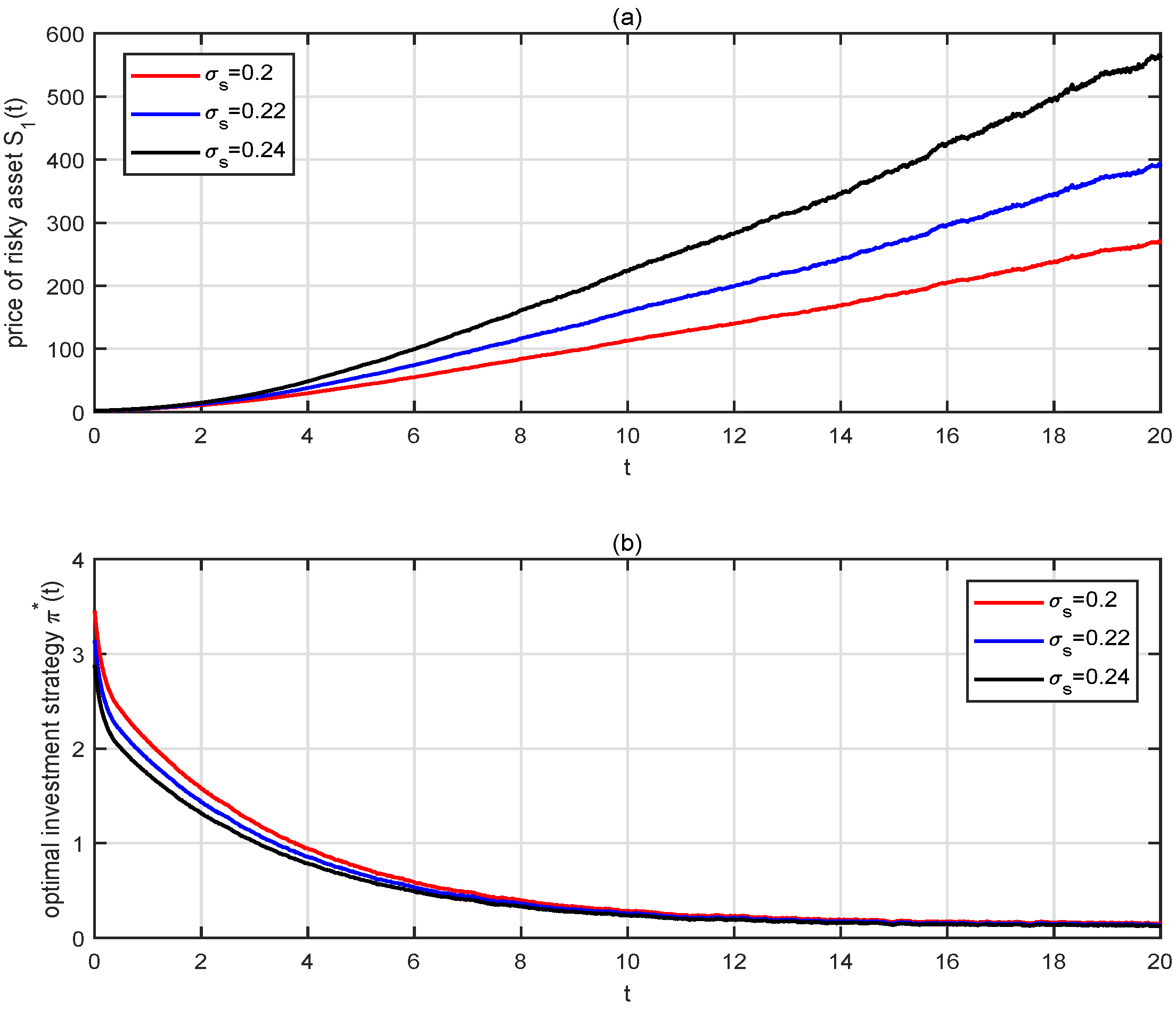
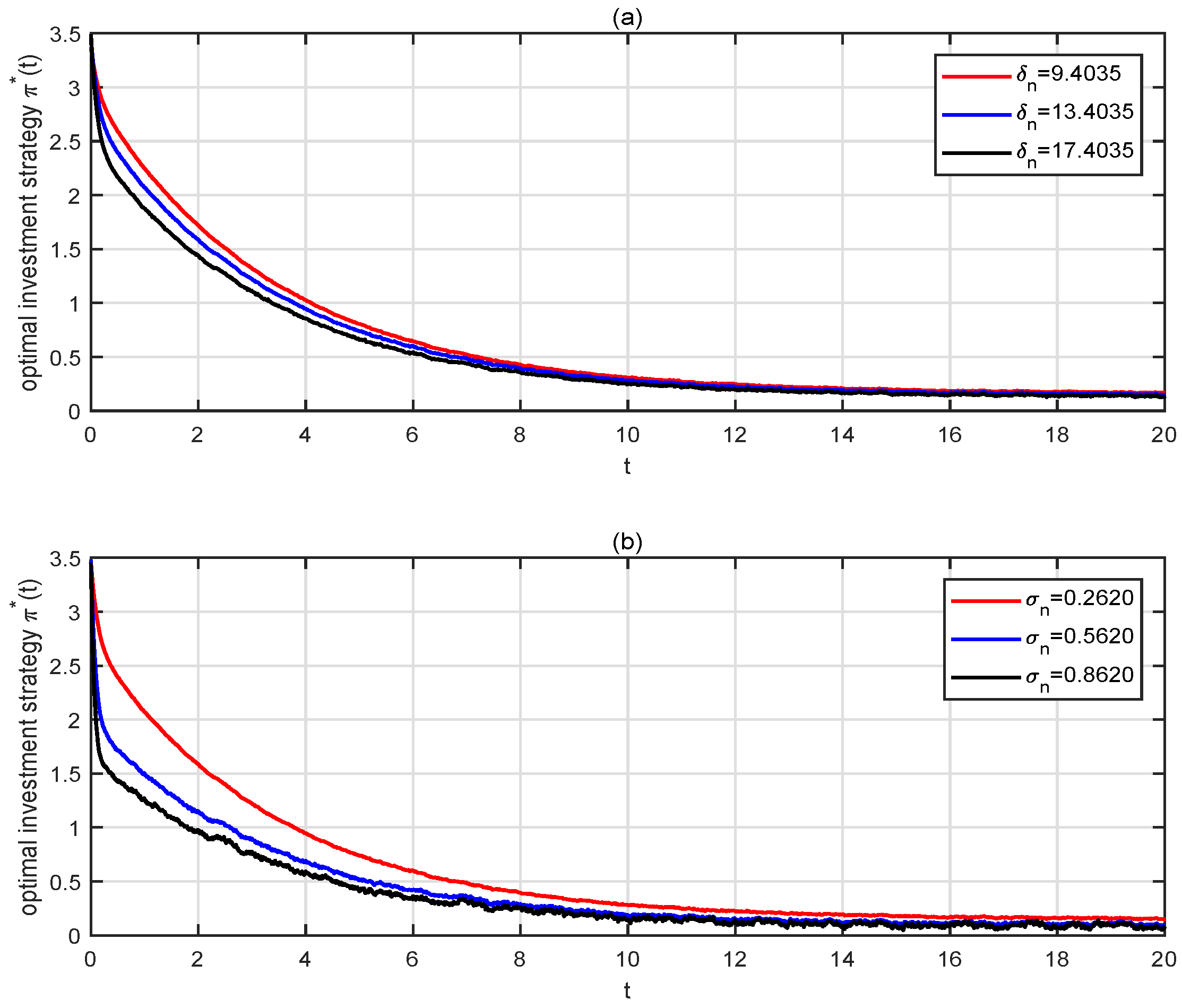
4.1. Numerical Results of the Optimal Investment Strategies

To provide a more intuitive and clear representation of how parameter changes affect decision-making, we focus on the range $t\in [0,20]$ since the curve’s trend remains relatively stable within this interval $t\in [20,40]$. For this purpose, we construct a Euler’s discretization scheme of Equation (3).

$$\left\{\begin{array}{cc}\hfill m_{(i+1)\Delta t}=& m_{i\Delta t}+k_m(\overline{m}-m_{i\Delta t})\Delta t+{\sigma }_m{p}_{ms}{\varphi }_1\sqrt{\Delta t}+{\sigma }_m{\overline{p}}_m{\varphi }_2\sqrt{\Delta t}.\hfill \\ \hfill {\widehat{n}}_{(i+1)\Delta t}=& {\widehat{n}}_{i\Delta t}+k_n(\overline{n}-{\widehat{n}}_{i\Delta t})\mathrm{d}t+({\sigma }_n{p}_{ns}+{\delta }_n{\mathsf{\Sigma }}_{i\Delta t}){\varphi }_1\sqrt{\Delta t}+({\sigma }_n{\overline{p}}_{nm}-\frac{{\delta }_n\mathsf{\Sigma }(t)p_{ms}}{{\overline{p}}_m}){\varphi }_2\sqrt{\Delta t}.\hfill \end{array}\right.$$

where $\Delta t$ is the finite timestep and ${\varphi }_1$ and ${\varphi }_2$ are two random numbers which are from the Gaussian law $N(0;1)$. Here, we note that it generates a new random number at each timestep. After i steps $(T=i\Delta t)$, we will obtain a single path.

Based on 1000 simulated sample paths for an investment strategy, we depict the average of the optimal investment strategy. Figure 1 reveals the difference between the optimal investment strategy under the stochastic volatility model and the constant volatility model, where the optimal investment strategy ${\pi }^{\ast }(t)$ corresponds to the original optimization problem with ${\sigma }_s=0.2$, whereas ${\widehat{\pi }}^{\ast }(t)$ corresponds to the optimization problem that specifies ${\sigma }_s(m(t))=\sqrt{m{(t)}^2+\epsilon }$. Here, we set $\epsilon =0.025$ and $\overline{m}=0$. We find that the chosen volatility specification yields optimal portfolios with properties that are consistent with properties of well-known stochastic volatility models. With the increase of time t, the investment strategies ${\pi }^{\ast }(t)$ and ${\widehat{\pi }}^{\ast }(t)$ decrease. The optimal investment proportion of risky assets under the stochastic volatility model is higher than that under the constant volatility model, which can be attributed to the stochastic volatility model being able to describe the fluctuation of risky assets in the financial market more accurately than the constant volatility model. Fund managers with more market information will allocate risky assets more actively and thus increase the investment proportion of risky assets.

${\sigma }_s$ represents the price volatility of risky assets. For the sake of convenience, in Figure 2 and the rest of the figures, we assume ${\sigma }_s(m(t))={\sigma }_s=0.2$. As depicted in Figure 2a, the price fluctuation of the risky asset with a low ${\sigma }_s$ level is more moderate compared to that with a high ${\sigma }_s$ level, which aligns with our intuitive expectations. In Figure 2b, we observe that ${\pi }^{\ast }(t)$ decreases as ${\sigma }_s$ increases. As ${\sigma }_s$ increases, the pension fund’s investment in the risky asset has to bear more risk, which reduces the attractiveness of investing in risky assets for the pension fund manager. Consequently, the fund manager prefers to adopt a relatively conservative investment strategy and reduces holdings of risky assets under such circumstances. In addition, as the final date approaches, the fund manager prudently lowers the proportion of assets invested in the risky asset to minimize investment risk, in alignment with the pension fund’s principles of prioritizing safe investments.

Figure 3 shows the effect of the mean reversion rate of the unobservable factor $k_n$ on ${\pi }^{\ast }(t)$. Note that the mean reversion phenomenon is not obvious when $n(0)\equiv \overline{n}\equiv 0$ (because the initial value of the unobservable factor is equal to its long-term mean). To show the effect of $k_n$ on $\widehat{n}(t)$, we assume $n(0)=0.1$ in Figure 3a. We find that the larger the $k_n$, the faster the $n(t)$ returns to the long-term mean $\overline{n}$. In addition, as the prediction error $\mathsf{\Sigma }(t)$ decreases with $k_n$, implying that the prediction of $\widehat{n}(t)$ is more accurate, more information about the Sharpe ratio can be obtained. The manager with more market information prefers to actively allocate assets to the risky asset, which is consistent with the curves shown in Figure 3b.

Figure 4 demonstrates the effect of the parameters ${\delta }_n$ and ${\sigma }_n$ on the optimal investment strategy ${\pi }^{\ast }(t)$. Here, ${\delta }_n$ weights the amount of unobservable information. The larger ${\delta }_n$ is, the less information is directly available. Although unobservable information can be predicted by a learning mechanism, there are still prediction errors $\mathsf{\Sigma }(t)$. The higher the proportion of unobservable factors, the relatively less market information the manager has and therefore the less confidence the manager has in the investment. As shown in Figure 4a, the manager tends to make more conservative and prudent investment decisions, reducing the proportion of assets invested in the risky asset. Figure 4b shows the negative relationship between ${\pi }^{\ast }(t)$ and ${\sigma }_n$. The volatility of the expected return and forecasting error $\mathsf{\Sigma }(t)$ both increase with ${\sigma }_n$. Therefore, the fund manager will reduce the amount of assets invested in the risky asset as ${\sigma }_n$ increases.

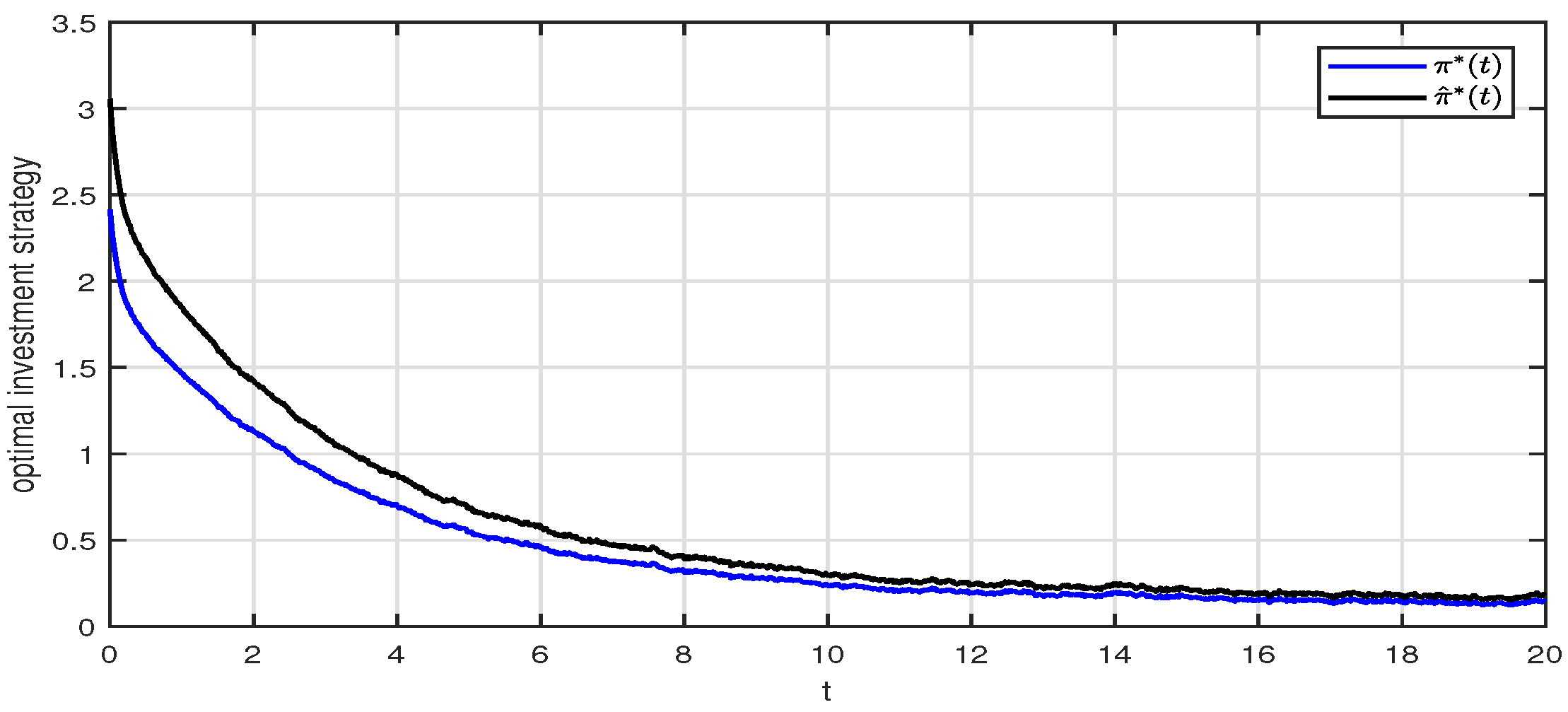
4.2. Comparison of the Optimal and Suboptimal Strategies

The optimal and suboptimal strategies have similar parameter structures as a result of the neglect of learning, as evidenced by Theorems 3 and 4. The primary difference between the two is whether the expected value is used or the filtered estimation of the unobservable state variable. The optimal asset allocation proportion ${\pi }^{\ast }(t)$ is compared to the suboptimal cases ${\tilde{\pi }}^{\ast }(t)$ in Figure 5, which does not account for learning. As shown in Figure 5, the general trends of the curves in both cases is almost the same, but ${\pi }^{\ast }(t)$ is usually higher than ${\tilde{\pi }}^{\ast }(t)$. It implies that a pension fund manager who is contemplating learning utilizes a greater amount of information when implementing policies, which enables the generation of more precise estimates of anticipated stock returns. Therefore, considering learning about stock returns becomes highly significant, particularly when dealing with a long investment period.

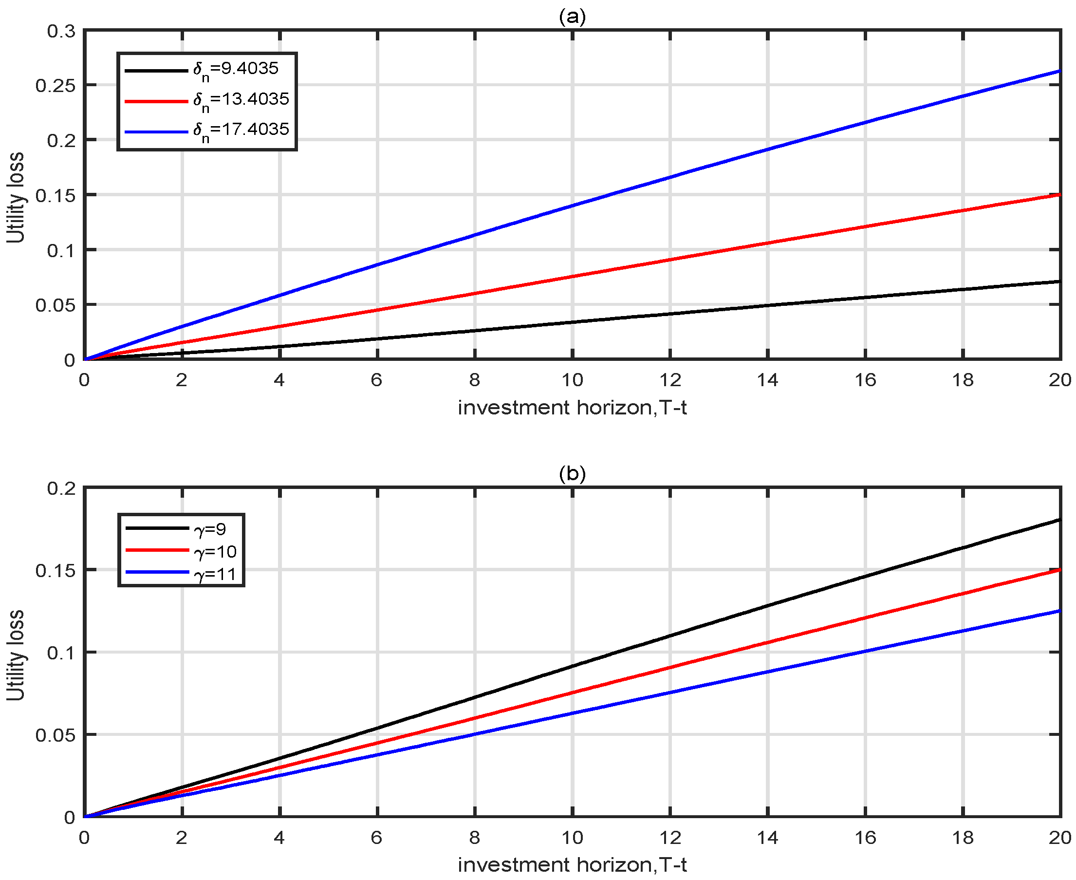
4.3. Analysis of Utility Losses from Ignoring Learning

Figure 6 illustrates the wealth-equivalent loss resulting from the suboptimal strategy, as determined by Equation (24), in order to evaluate the significance of learning. The loss function in Figure 6a exhibits a consistent upward trajectory as ${\delta }_n$ rises. The expected return of the stock is significantly influenced by the predictive power ${\delta }_n$, which is why it is increasingly important to understand about $n(t)$. Additionally, neglecting learning results in a greater utility loss over time, which diminishes as the risk aversion coefficient $\gamma$ rises in Figure 6b. Consequently, the disregard of learning will lead to a greater loss of utility.

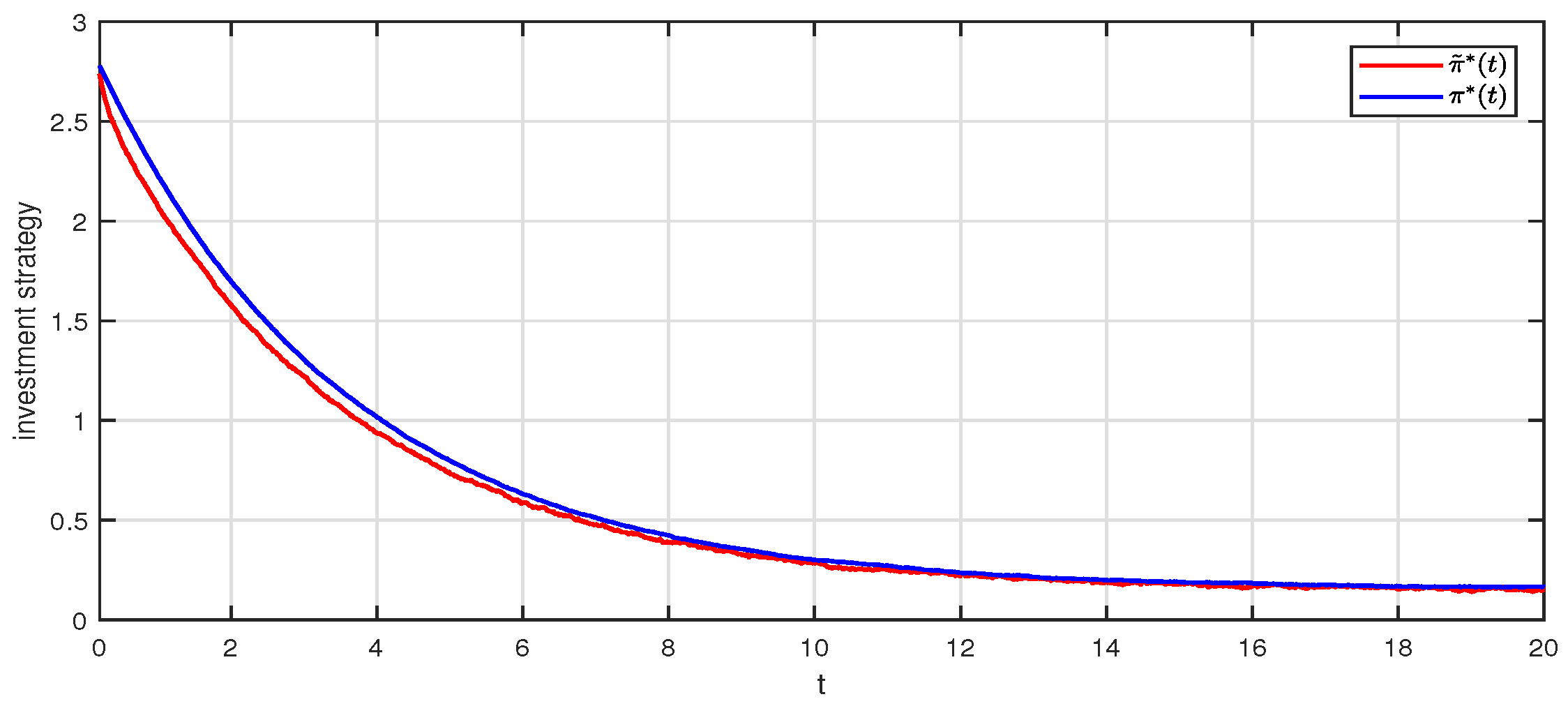
4.4. Effect of the Return of Premium Clause on the Optimal Investment Strategy

To analyze the impact of the return of premium clause on the amount of pension fund wealth, we denote the fund wealth with and without the clause by $X^{\ast }(t)$ and ${\widehat{X}}^{\ast }(t)$, respectively. $X^{\ast }(t)-{\widehat{X}}^{\ast }(t)$ represents the deviation of the above-mentioned two kinds of wealth. Figure 7 shows that the amount of fund wealth with the return of premium clause is lower than that without. The return of premium clause of the DC pension plan safeguards the rights of participants who pass away prior to retirement by permitting beneficiaries to withdraw the deceased’s pension contributions. This withdrawal mechanism results in a lower wealth level of pension funds than that without the return of premium clause. In addition, we find that the deviation amplifies over time, which is attributed to the probability of participants’ death increasing over time, leading to an increasing amount of wealth withdrawn from the pension fund. Moreover, Figure 7 depicts the impact of the risk aversion coefficient $\gamma$ of the fund manager on fund wealth. The lower the level of $\gamma$ is, the less risk averse the fund manager is and the more likely the manager is to implement more aggressive portfolio decisions. Thus, the relatively aggressive ($\gamma =$ 9) investment strategy may incur greater wealth deviation.

5. Conclusions

This paper delves into the optimal investment strategy for DC pension funds by incorporating partial information and a return of premium clause. Our study considers a financial market with both risk-free and risky assets. In our model, the fund manager observes just the stock price but not the appreciation rate. Utilizing Kalman filter theory, we predict unobservable information. Furthermore, we integrate the return of premium clause into the continuous-time optimization framework, allowing beneficiaries to withdraw the pension wealth accumulated by participants who passed away before retirement. By aiming to maximize the expected utility of the pension fund at the terminal time, we construct a stochastic optimal control problem and derive the optimal asset-allocation strategy.

We conclude that (1) learning impacts the level and structure of the optimal demand for the stock; fund managers who have more market information prefer to allocate wealth to risky assets; (2) neglecting learning can lead to economically significant losses, particularly when dealing with a long investment period; (3) the wealth of pension funds with return of premium clauses is lower than those without such clauses and the wealth deviation will also gradually expand because the probability of participants’ death increases with age. Thus, it is very important to consider the learning mechanism and return of premium clause for a DC pension plan with a long investment period.

In future research, we will study the optimal investment of DC pension fund managers with loss aversion preferences based on the cumulative prospect theory in partial information behavioral finance. The S-shaped utility function corresponding to loss aversion is more appropriate in describing the behavioral characteristics and risk preferences of pension fund managers. Therefore, it may be useful to combine partial information with loss aversion to obtain the optimal investment of DC pension funds.

References

1. Li, D.; Ng, W.L. Optimal dynamic portfolio selection: Multiperiod mean-variance formulation. Math. Financ. 2000, 10, 387–406. [Google Scholar] [CrossRef]
2. Xiao, H.; Zhou, Z.; Ren, T.; Bai, Y.; Liu, W. Time-consistent strategies for multi-period mean-variance portfolio optimization with the serially correlated returns. Commun.-Stat.-Theory Methods 2020, 49, 2831–2868. [Google Scholar] [CrossRef]
3. Battocchio, P.; Menoncin, F. Optimal pension management in a stochastic framework. Insur. Math. Econ. 2004, 34, 79–95. [Google Scholar] [CrossRef]
4. Han, N.; Hung, M. Optimal asset allocation for DC pension plans under inflation. Insur. Math. Econ. 2012, 51, 172–181. [Google Scholar] [CrossRef]
5. Zeng, Y.; Li, D.; Chen, Z.; Yang, Z. Ambiguity aversion and optimal derivative-based pension investment with stochastic income and volatility. J. Econ. Dyn. Control 2018, 88, 70–103. [Google Scholar] [CrossRef]
6. Wang, P.; Li, Z.; Sun, J. Robust portfolio choice for a DC pension plan with inflation risk and mean-reverting risk premium under ambiguity. Optimization 2021, 70, 191–224. [Google Scholar] [CrossRef]
7. Wang, P.; Li, Z. Robust optimal investment strategy for an AAM of DC pension plans with stochastic interest rate and stochastic volatility. Insur. Math. Econ. 2018, 80, 67–83. [Google Scholar] [CrossRef]
8. Dong, Y.; Zheng, H. Optimal investment of DC pension plan under shortselling constraints and portfolio insurance. Insur. Math. Econ. 2019, 85, 47–59. [Google Scholar] [CrossRef]
9. Lv, W.; Tian, L.; Zhang, X. Optimal Defined Contribution Pension Management with Jump Diffusions and Common Shock Dependence. Mathematics 2023, 11, 2954. [Google Scholar] [CrossRef]
10. He, L.; Liang, Z. Optimal investment strategy for the DC plan with the return of premiums clauses in a mean–variance framework. Insur. Math. Econ. 2013, 53, 643–649. [Google Scholar] [CrossRef]
11. Bian, L.; Li, Z.; Yao, H. Pre-commitment and equilibrium investment strategies for the DC pension plan with regime switching and a return of premiums clause. Insur. Math. Econ. 2018, 81, 78–94. [Google Scholar] [CrossRef]
12. Chang, H.; Li, J. Robust equilibrium strategy for DC pension plan with the return of premiums clauses in a jump-diffusion model. Optimization 2023, 72, 463–492. [Google Scholar] [CrossRef]
13. Li, D.; Rong, X.; Zhao, H.; Yi, B. Equilibrium investment strategy for DC pension plan with default risk and return of premiums clauses under CEV model. Insur. Math. Econ. 2017, 72, 6–20. [Google Scholar] [CrossRef]
14. Lai, C.; Liu, S.; Wu, Y. Optimal portfolio selection for a defined-contribution plan under two administrative fees and return of premium clauses. J. Comput. Appl. Math. 2021, 398, 113694. [Google Scholar] [CrossRef]
15. Nie, G.; Chen, X.; Chang, H. Time-consistent strategies between two competitive DC pension plans with the return of premiums clauses and salary risk. Commun. Stat.-Theory Methods 2023, 1–22. [Google Scholar] [CrossRef]
16. Fama, E.; French, K. Permanent and temporary components of stock prices. J. Political Econ. 1988, 96, 246–273. [Google Scholar] [CrossRef]
17. Boudoukh, J.; Michaely, R.; Richardson, M.; Roberts, M. On the importance of measuring payout yield: Implications for empirical asset pricing. J. Financ. 2007, 62, 877–915. [Google Scholar] [CrossRef]
18. Brennan, M. The role of learning in dynamic portfolio decisions. Rev. Financ. 1998, 1, 295–306. [Google Scholar] [CrossRef]
19. Van Binsbergen, J.; Koijen, R. Predictive regressions: A present-value approach. J. Financ. 2010, 65, 1439–1471. [Google Scholar] [CrossRef]
20. Branger, N.; Larsen, L.; Munk, C. Robust portfolio choice with ambiguity and learning about return predictability. J. Bank. Financ. 2013, 37, 1397–1411. [Google Scholar] [CrossRef]
21. Escobar, M.; Ferrando, S.; Rubtsov, A. Portfolio choice with stochastic interest rates and learning about stock return predictability. Int. Rev. Econ. Financ. 2016, 41, 347–370. [Google Scholar] [CrossRef]
22. Wang, P.; Shen, Y.; Zhang, L.; Kang, Y. Equilibrium investment strategy for a DC pension plan with learning about stock return predictability. Insur. Math. Econ. 2021, 100, 384–407. [Google Scholar] [CrossRef]
23. Xia, Y. Learning about predictability: The effects of parameter uncertainty on dynamic asset allocation. J. Financ. 2001, 56, 205–246. [Google Scholar] [CrossRef]
24. Huang, J.; Chen, Z. Optimal risk asset allocation of a loss-averse bank with partial information under inflation risk. Financ. Res. Lett. 2021, 38, 101513. [Google Scholar] [CrossRef]
25. Wang, P.; Zhang, L.; Li, Z. Asset allocation for a DC pension plan with learning about stock return predictability. J. Ind. Manag. Optim. 2022, 18, 3847–3877. [Google Scholar] [CrossRef]
26. Harvey, C. The specification of conditional expectations. J. Empir. Financ. 2001, 8, 573–637. [Google Scholar] [CrossRef]
27. Whitelaw, R. Time variations and covariations in the expectation and volatility of stock market returns. J. Financ. 1994, 49, 515–541. [Google Scholar] [CrossRef]
28. Chacko, G.; Viceira, L. Dynamic consumption and portfolio choice with stochastic volatility in incomplete markets. Rev. Financ. Stud. 2005, 18, 1369–1402. [Google Scholar] [CrossRef]
29. Liptser, R.; Shiryaev, A. Statistics of Random Processes. Volume 2: Applications; Springer: Heidelberg/Berlin, Germany, 2001. [Google Scholar]
30. Fleming, W.; Soner, H. Controlled Markov Processes and Viscosity Solutions; Springer Science and Business Media: Berlin/Heidelberg, Germany, 2006; Volume 25. [Google Scholar]
31. Heston, S. A closed-form solution for options with stochastic volatility with applications to bonds and currency options. Rev. Financ. Stud. 1993, 6, 327–343. [Google Scholar] [CrossRef]
32. Larsen, L.S.; Munk, C. The costs of suboptimal dynamic asset allocation: General results and applications to interest rate risk, stock volatility risk and growth/value tilts. J. Econ. Dyn. Control. 2012, 36, 266–293. [Google Scholar] [CrossRef]
33. Flor, C.; Larsen, L. Robust portfolio choice with stochastic interest rates. Ann. Financ. 2014, 10, 243–265. [Google Scholar] [CrossRef]
Figure 1. The optimal investment strategies.
Mathematics 12 02130 g001
Figure 2. (a) The effect of σ s on the price of the risky asset S 1 ( t ) ; (b) The effect of σ s on the optimal investment strategy π ( t ) .
Mathematics 12 02130 g002
Figure 3. (a) The effect of k n on the adapted filter n ^ ( t ) ; (b) The effect of k n on the optimal investment strategy π ( t ) .
Mathematics 12 02130 g003
Figure 4. (a) The effect of δ n on the optimal investment strategy π ( t ) ; (b)The effect of σ n on the optimal investment strategy π ( t ) .
Mathematics 12 02130 g004
Figure 5. Comparison of the optimal strategy π ( t ) and the suboptimal strategy π ˜ ( t ) when ignoring learning.
Mathematics 12 02130 g005
Figure 6. (a) The utility loss functions for δ n ; (b) The utility loss functions for γ .
Mathematics 12 02130 g006
Figure 7. The effect of γ on the optimal investment strategy.
Mathematics 12 02130 g007