
Updating Correlation-Enhanced Feature Learning for Multi-Label Classification


Abstract
:1. Introduction
- Our method distinguishes itself from the preponderance of multi-label correlation learning algorithms by directly extracting label correlations from the data itself, thereby enhancing their precision beyond those derived solely from pre-assigned labels.
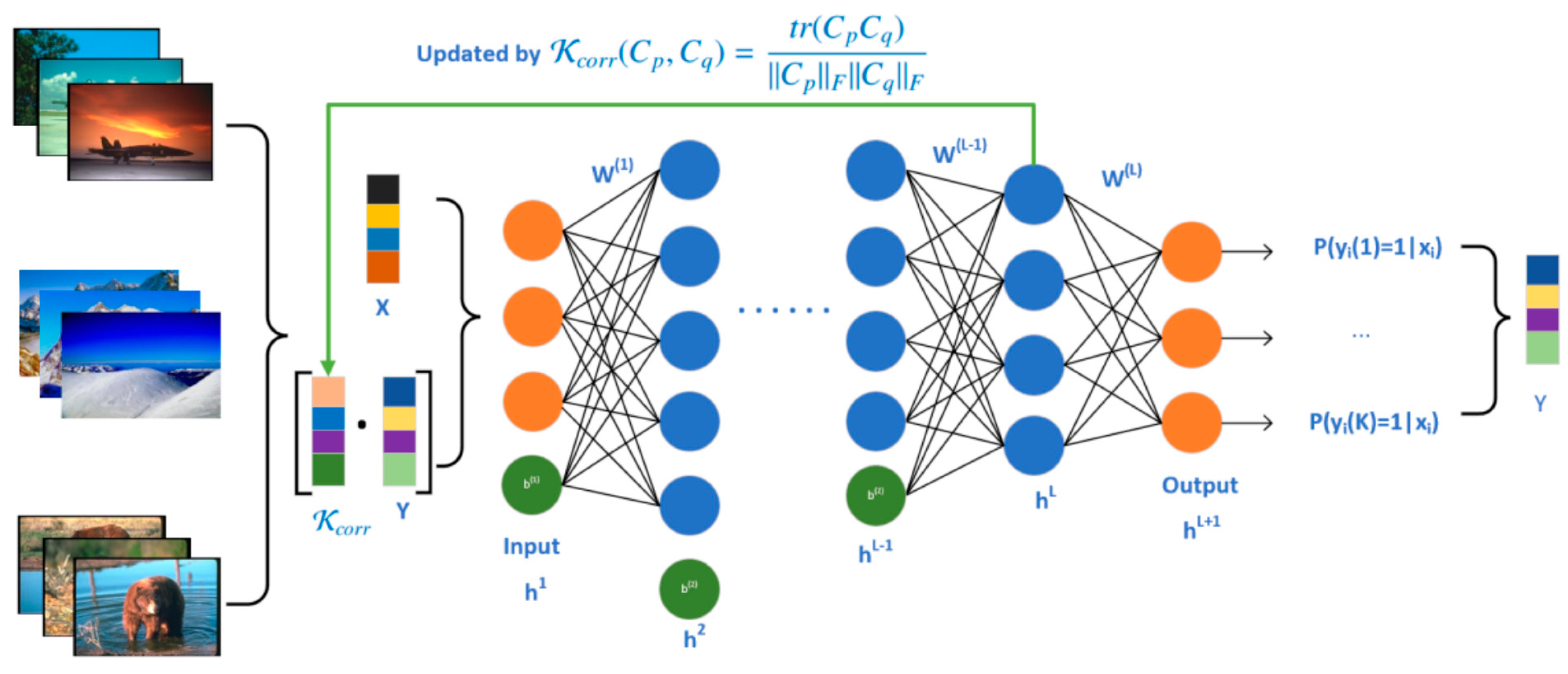
- We introduce a revised label matrix, obtained by multiplying the incomplete label matrix with the captured label correlation, which serves to enrich the original data’s feature representation. A multi-layer neural network is then employed to learn the correlation-enhanced features that encapsulate intricate relationships among data features, labels, and their interconnections.
- Leveraging the high-level semantic features extracted by the multi-layer neural network, our uCeFL approach re-evaluates the label correlation, facilitating continuous updates of these correlations throughout the neural network’s learning trajectory. This approach effectively captures the label propagation effects, ensuring a comprehensive and accurate representation of the label space.
2. The Related Work
3. Algorithm Description
3.1. Motivation
3.2. The Proposed CeFL
| Algorithm 1: uCeFL |
| Input: , ; Output: . 1. with appropriate values; 2. FirstFlag = true; 3. for each label k do 4. Construct the subset of training data associated with label k as ; 5. end for 6. for t = 1, 2, … T do 7. for each label k do 8. if FirstFlag = false then 9. ; 10. ; 11. ; 12. else 13. ; 14. FirstFlag = false; 15. end if 16. Compute covariance matrix of each ; 17. end for 18. Calculate the Covariance Matrix Similarity Coefficient by Equation (2); 19. Train the neural network using as input, then update and ; 20. if or then 21. Turn to return; 22. end if 23. end for 24. return Parameters and . |
| Algorithm 2: CeFL |
| Input: Training data matrix , label matrix , network layer number , iterative number , convergence error ; Output: Parameters and . 1. Initialize and with appropriate values; 2. for each label do 3. Construct the subset of training data associated with label as ; 4. Compute the covariance matrix of matrix ; 5. end for 6. Calculate the Covariance Matrix Similarity Coefficient by Equation (2); 7. for do 8. Train the neural network using as input, then update and ; 9. if or then 10. Turn to return; 11. end if 12. end for 13. return Parameters and . |
4. Experiments
4.1. Experimental Criteria
- HammingLoss is an example-based multi-label classification evaluation criterion that indicates the proportion of misclassified instances in two scenarios: when predicted labels do not belong to the instance, and when labels belonging to the instance are not predicted,where indicates the symmetric difference between the predicted and actual label vectors for each instance.
- SubsetAccuracy is a measure of classification accuracy. It considers a classification to be correct when the set of predicted labels exactly matches the set of true labels, and incorrect otherwise. Specifically, SubsetAccuracy calculates the proportion of instances in the test set that are fully and accurately classified,where is the indicator function. This metric provides a holistic view of the performance of a classification model with respect to predicting entire sets of labels, rather than just individual labels.
- Accuracy is the ratio of correctly predicted labels to the total number of predicted labels:
- F1Measure is a comprehensive evaluation index that combines precision and recall, and is also referred to as the comprehensive classification rate. The precision rate measures how many of the predicted labels are actually correct,The recall rate is the ratio of correctly predicted positive labels to the total number of actual positive labels,The F1Measure isThese evaluation metrics are example-based. We also consider label-based evaluation metrics, which are widely used in the literature. Let , , , and represent the number of true positives, true negatives, false positives, and false negatives, respectively, for label .
- MacroF1Measure is the arithmetic average value of the F1Measure of all labels.
- MicroF1Measure sums the Precisionj and Recallj of all labels before calculating the F1measure.For all these metrics except HammingLoss, a larger value indicates better classifier performance.
4.2. Implementation Details
4.3. Performance Comparison and Discussion
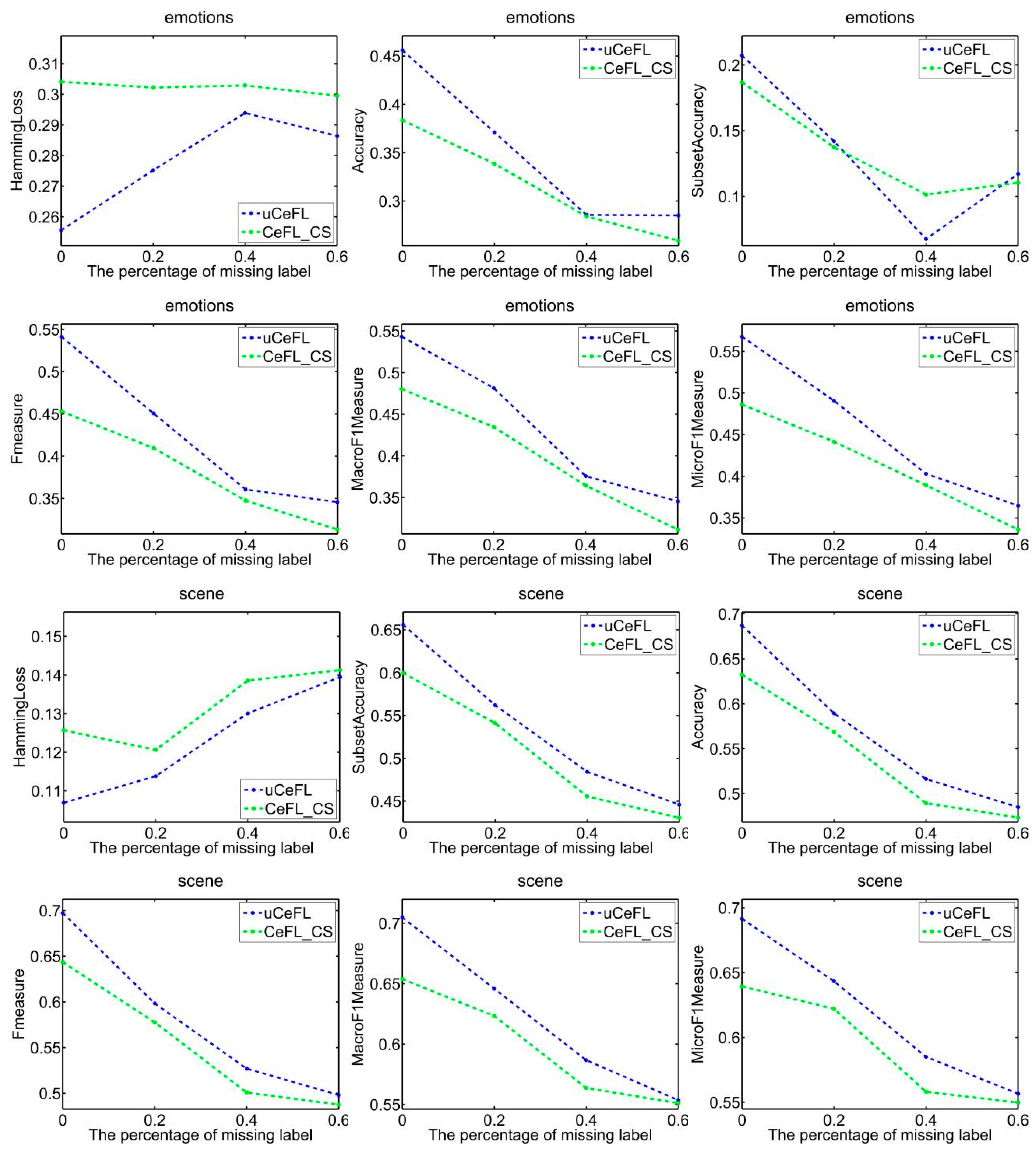
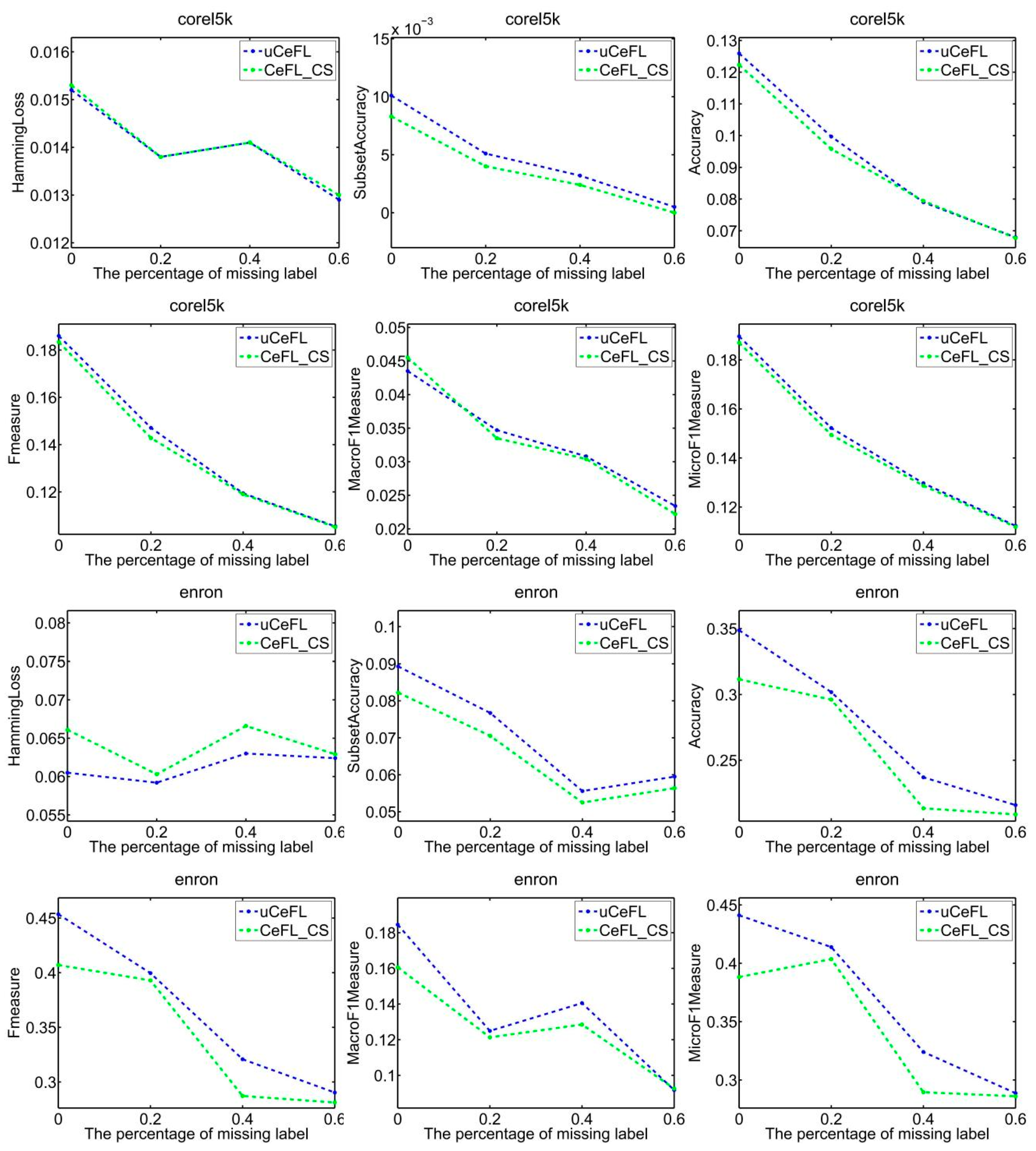
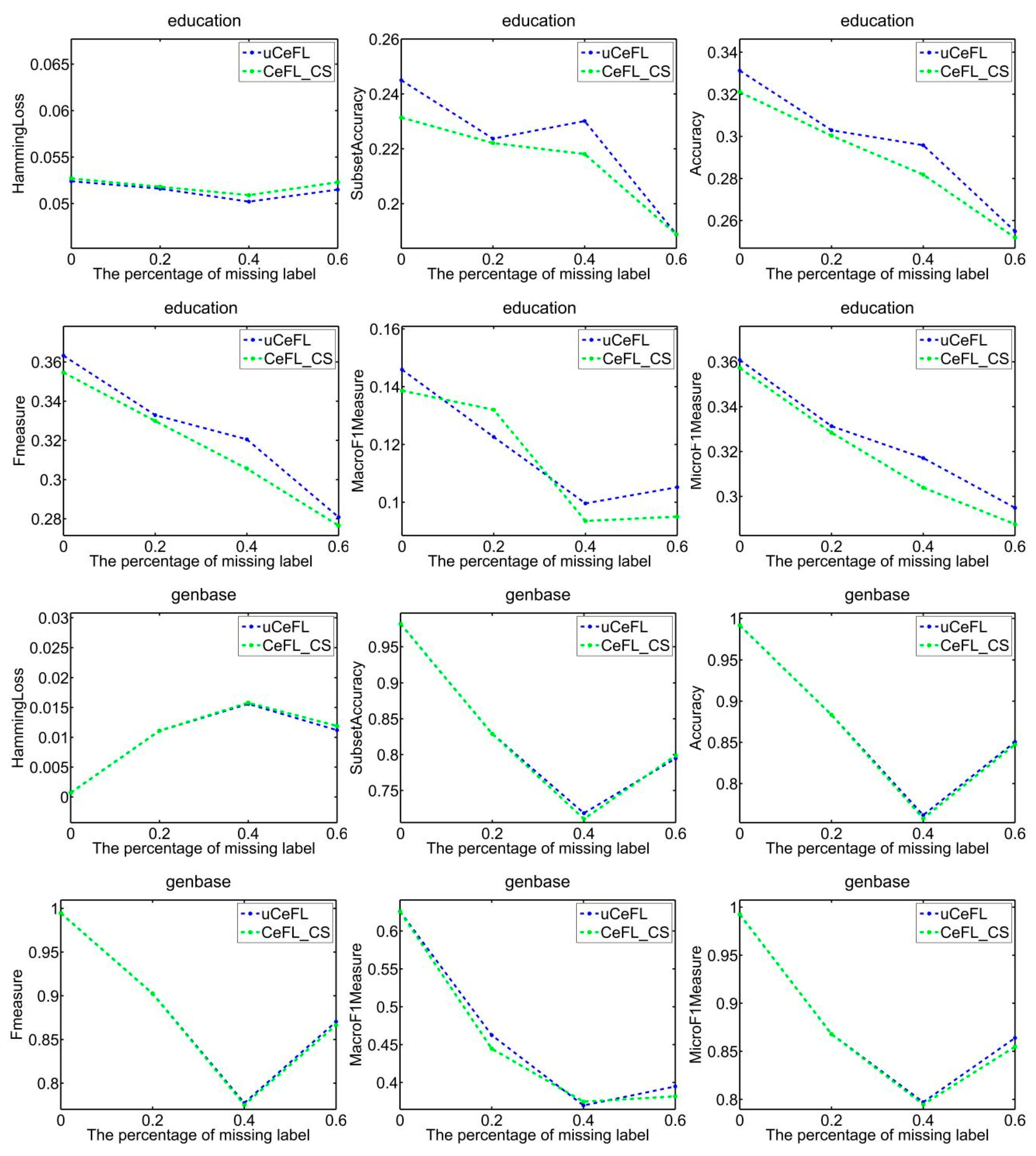
- Overall, uCeFL was obviously competitive with the comparison approaches, especially on the emotions, genbase, medical, and corel5k datasets, where uCeFL performed best, regardless of the loss rate.
- When the label is not missing, TRAM performs relatively well on the three scene, enron, and education databases, and its performance on the other four datasets is also quite competitive. However, it is crucial to note that in the step of deriving the transformation matrix P, there is a significant reliance on the sample ground-truth labels. If labels are missing in the dataset, the accuracy of the obtained transformation matrix P may be compromised, potentially leading to inaccuracies in the labeling of unlabeled samples. Consequently, as the rate of missing labels increases, the overall performance of the system declines accordingly.
- ML-KNN only performed well on the scene dataset, and its performance was optimal when the missing rate was 0.2. ML-KNN utilizes the label information of the k-nearest neighbors of the test data to estimate the label set, but it does not take into account label correlation. Therefore, poor label annotation performance is possible when some class labels of the training data are missing.
- Similar to our approaches, the label space is augmented in LLSF-DL with the feature space as additional features. LLSF-DL removes unnecessary dependency relationships by identifying the sparsity coefficient of the label space . However, it may disregard correct indirect relationships resulting from labels that are not subject to sparsity coefficient consideration, which could be a reason why its performance is not ideal.
- Compared to LCFM, which tackles missing labels by integrating both global and local label-specific features, our method leverages neural networks with hidden layers. This facilitates hierarchical learning of label-expanded data features and adeptly extracts high-level semantic features from the data. These features capture three distinct relationships: between data features, between labels and data features, and among labels. Experimental results confirm that these features offer significant benefits for the development of subsequent classification models.
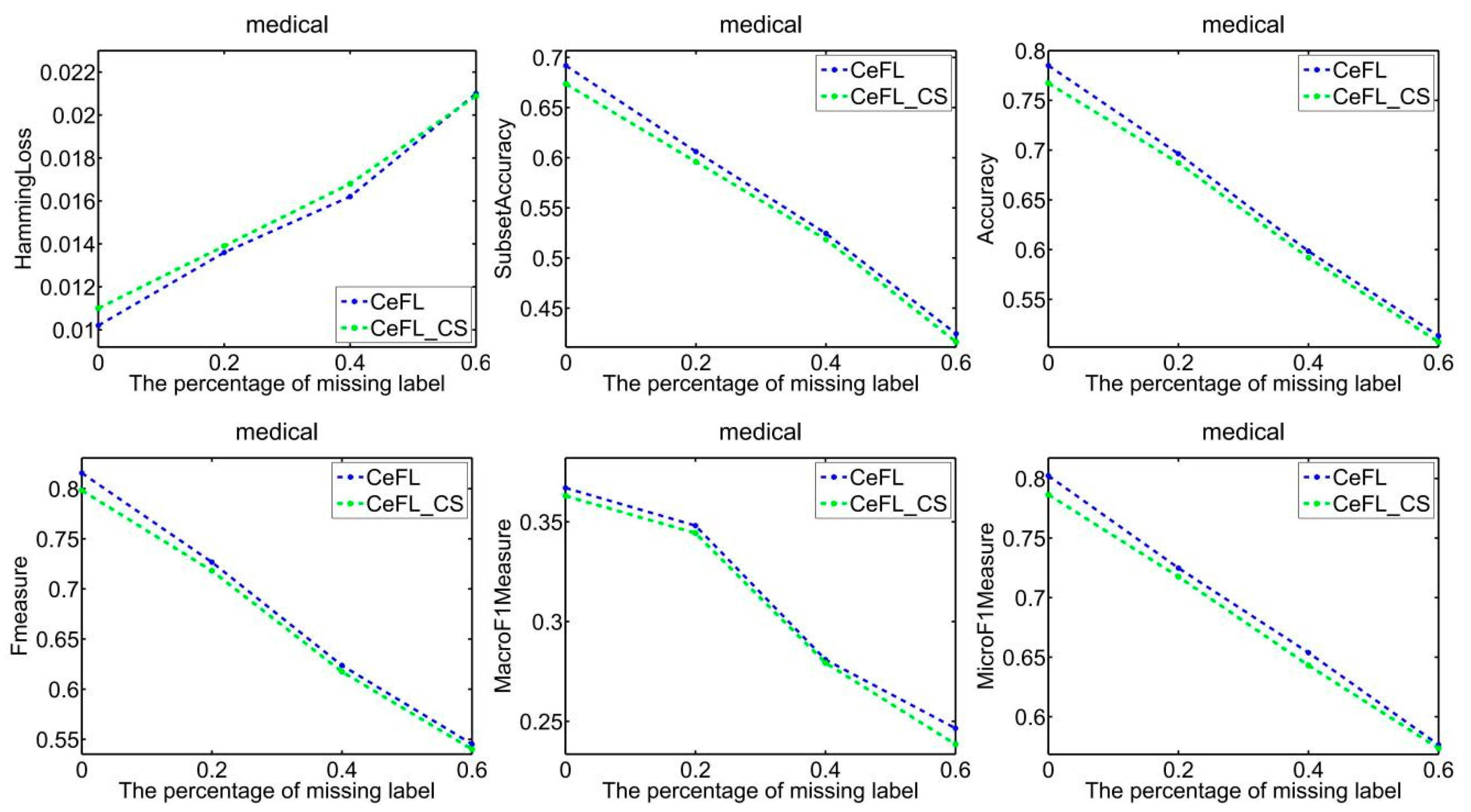
- At the end of each round of training, uCeFL performs a feedforward process to extract high-level features from the input data. Label correlations are then recalculated to update the input for the next round of training. Therefore, uCeFL not only takes the label correlations as prior knowledge but also continuously improves them during the learning process of the classification model. The experimental results show that uCeFL works better than CeFL, which demonstrates the effectiveness of using neural networks with hidden layers for feature learning.
5. Conclusions and Future Works
- This paper employed a covariance matrix to represent the dataset comprising category labels and derived label correlations through the calculation of a covariance matrix similarity coefficient. However, computing these correlations becomes challenging when dealing with a substantial data volume. The issue of efficiently acquiring label correlations in a big-data environment demands further exploration.
- Moreover, the paper only concentrated on one-to-one label correlations. To accurately capture the actual label correlations, further research is needed, encompassing investigations into both local and global correlations.
- The presence of multi-label data introduces the curse of dimensionality. Future aims can explore the relationship between labels and features to identify a more discriminative subspace.
Author Contributions
Funding
Data Availability Statement
Conflicts of Interest
References
- Shu, X.; Qiu, J. Speed up kernel dependence maximization for multi-label feature extraction. J. Vis. Commun. Image Represent. 2017, 49, 361–370. [Google Scholar] [CrossRef]
- Du, J.; Chen, Q.; Peng, Y.; Xiang, Y.; Tao, C.; Lu, Z. Ml-net: Multi-label classification of biomedical texts with deep neural networks. J. Am. Med. Inform. Assoc. 2019, 26, 1279–1285. [Google Scholar] [CrossRef]
- Wang, T.; Liu, L.; Liu, N.; Zhang, H.; Zhang, L.; Feng, S. A multi-label text classification method via dynamic semantic representation model and deep neural network. Appl. Intell. 2020, 50, 2339–2351. [Google Scholar] [CrossRef]
- Tang, R.; Yu, Z.; Ma, Y.; Wu, Y.; Chen, Y.-P.P.; Wong, L.; Li, J. Genetic source completeness of hiv-1 circulating recombinant forms (crfs) predicted by multi-label learning. Bioinformatics 2020, 37, 750–758. [Google Scholar] [CrossRef] [PubMed]
- Zhou, Z.; Waqas, J. Intrinsic structure based feature transform for image classification. J. Vis. Commun. Image Represent. 2016, 38, 735–744. [Google Scholar] [CrossRef]
- Gou, J.; Song, J.; Ou, W.; Zeng, S.; Yuan, Y.; Du, L. Representation-based classification methods with enhanced linear reconstruction measures for face recognition. Comput. Electr. Eng. 2019, 79, 106451. [Google Scholar] [CrossRef]
- Zhang, Y.; Zhou, Z.-H. Multilabel dimensionality reduction via dependence maximization. ACM Trans. Knowl. Discov. Data 2010, 4, 1–21. [Google Scholar] [CrossRef]
- Li, Y.-K.; Zhang, M.-L. Enhancing binary relevance for multi-label learning with controlled label correlations exploitation. In Pacific Rim International Conference on Artificial Intelligence; Springer: Cham, Switzerland, 2014; pp. 91–103. [Google Scholar] [CrossRef]
- Xu, L.; Wang, Z.; Shen, Z.; Wang, Y.; Chen, E. Learning low-rank label correlations for multi-label classification with missing labels. In Proceedings of the 2014 IEEE International Conference on data Mining, Shenzhen, China, 14–17 December 2014; IEEE: New York, NY, USA, 2014; pp. 1067–1072. [Google Scholar] [CrossRef]
- Tsoumakas, G.; Katakis, I. Multi-label classification: An overview. Int. J. Data Warehous. Min. 2007, 3, 1–13. [Google Scholar] [CrossRef]
- Read, J.; Pfahringer, B.; Holmes, G. Multi-label classification using ensembles of pruned sets. In Proceedings of the 2008 Eighth IEEE International Conference on Data Mining, Pisa, Italy, 15–19 December 2008; IEEE: New York, NY, USA, 2008; pp. 995–1000. [Google Scholar] [CrossRef]
- Tsoumakas, G.; Vlahavas, I. Random k-labelsets: An ensemble method for multilabel classification. In European Conference on Machine Learning; Springer: Berlin/Heidelberg, Germany, 2007; pp. 406–417. [Google Scholar] [CrossRef]
- Wang, C.; Yan, S.; Zhang, L.; Zhang, H.-J. Multi-label sparse coding for automatic image annotation. In Proceedings of the 2009 IEEE Conference on Computer Vision and Pattern Recognition, Miami, FL, USA, 20–25 June 2009; IEEE: New York, NY, USA, 2009; pp. 1643–1650. [Google Scholar] [CrossRef]
- Wang, H.; Huang, H.; Ding, C. Image annotation using multi-label correlated green’s function. In Proceedings of the 2009 IEEE 12th International Conference on Computer Vision, Kyoto, Japan, 27 September–4 October 2009; IEEE: New York, NY, USA, 2009; pp. 2029–2034. [Google Scholar] [CrossRef]
- Huang, S.-J.; Zhou, Z.-H. Multi-label learning by exploiting label correlations locally. In Proceedings of the AAAI Conference on Artificial Intelligence, Toronto, ON, USA, 22–26 July 2012; Volume 26. [Google Scholar] [CrossRef]
- Gu, Q.; Li, Z.; Han, J. Correlated multi-label feature selection. In Proceedings of the 20th ACM International Conference on Information and Knowledge Management, Glasgow UK, 24–28 October 2011; pp. 1087–1096. [Google Scholar] [CrossRef]
- Ji, S.; Tang, L.; Yu, S.; Ye, J. Extracting shared subspace for multi-label classification. In Proceedings of the 14th ACM SIGKDD International Conference on Knowledge Discovery and Data Mining, Las Vegas, NV, USA, 24–27 August 2008; pp. 381–389. [Google Scholar] [CrossRef]
- Read, J.; Pfahringer, B.; Holmes, G.; Frank, E. Classifier chains for multi-label classification. Mach. Learn. 2011, 85, 333–359. [Google Scholar] [CrossRef]
- Montañes, E.; Senge, R.; Barranquero, J.; Quevedo, J.R.; del Coz, J.J.; Hüllermeier, E. Dependent binary relevance models for multi-label classification. Pattern Recognit. 2014, 47, 1494–1508. [Google Scholar] [CrossRef]
- Huang, J.; Qin, F.; Zheng, X.; Cheng, Z.; Yuan, Z.; Zhang, W.; Huang, Q. Improving multi-label classification with missing labels by learning label-specific features. Inf. Sci. 2019, 492, 124–146. [Google Scholar] [CrossRef]
- Zhu, P.; Xu, Q.; Hu, Q.; Zhang, C.; Zhao, H. Multi-label featureselection with missing labels. Pattern Recognit. 2018, 74, 488–502. [Google Scholar] [CrossRef]
- Rauber, T.W.; Mello, L.H.; Rocha, V.F.; Luchi, D.; Varejão, F.M. Recursive dependent binary relevance model for multi-label classification. In Advances in Artificial Intelligence–IBERAMIA 2014: 14th Ibero-American Conference on AI, Santiago de Chile, Chile, 24–27 November 2014; Proceedings 14; Springer: Cham, Switzerland, 2014; pp. 206–217. [Google Scholar] [CrossRef]
- Zhang, Y.; Li, Y.; Cai, Z. Correlation-based pruning of dependent binary relevance models for multi-label classification. In Proceedings of the 2015 IEEE 14th International Conference on Cognitive Informatics & Cognitive Computing (ICCICC), Beijing, China, 6–8 July 2015; IEEE: New York, NY, USA, 2015. [Google Scholar] [CrossRef]
- Rauber, T.W.; Rocha, V.F.; Mello, L.H.S.; Varejao, F.M. Decision template multi-label classification based on recursive dependent binary relevance. In Proceedings of the 2016 IEEE Congress on Evolutionary Computation (CEC), Vancouver, BC, Canada, 24–29 July 2016; IEEE: New York, NY, USA, 2016; pp. 2402–2408. [Google Scholar] [CrossRef]
- Zhang, M.L.; Wu, L. Lift: Multi-label learning with label-specific features. IEEE Trans. Pattern Anal. Mach. Intell. 2014, 37, 107–120. [Google Scholar] [CrossRef] [PubMed]
- Zhang, J.-J.; Fang, M.; Li, X. Multi-label learning with discriminative features for each label. Neurocomputing 2015, 154, 305–316. [Google Scholar] [CrossRef]
- Xu, S.; Yang, X.; Yu, H.; Yu, D.-J.; Yang, J.; Tsang, E.C. Multi-label learning with label-specific feature reduction. Knowl. Based Syst. 2016, 104, 52–61. [Google Scholar] [CrossRef]
- Lee, J.; Kim, D.-W. Efficient multi-label feature selection using entropy-based label selection. Entropy 2016, 18, 405. [Google Scholar] [CrossRef]
- Mencía, E.L.; Janssen, F. Learning rules for multi-label classification: A stacking and a separate-and-conquer approach. Mach. Learn. 2016, 105, 77–126. [Google Scholar] [CrossRef]
- Li, Q.; Peng, X.; Qiao, Y.; Peng, Q. Learning label correlations for multi-label image recognition with graph networks. Pattern Recognit. Lett. 2020, 138, 378–384. [Google Scholar] [CrossRef]
- RWang, R.; Ye, S.; Li, K.; Kwong, S. Bayesian network based label correlation analysis for multi-label classifier chain. Inf. Sci. 2020, 554, 256–275. [Google Scholar] [CrossRef]
- Zhan, W.; Zhang, M.-L. Multi-label learning with label-specific features via clustering ensemble. In Proceedings of the 2017 IEEE International Conference on Data Science and Advanced Analytics (DSAA), Tokyo, Japan, 19–21 October 2017; IEEE: New York, NY, USA, 2017; pp. 129–136. [Google Scholar] [CrossRef]
- Zhang, J.; Li, C.; Cao, D.; Lin, Y.; Su, S.; Dai, L.; Li, S. Multi-label learning with label-specific features by resolving label correlations. Knowl. Based Syst. 2018, 159, 148–157. [Google Scholar] [CrossRef]
- Liu, H.; Ma, Z.; Han, J.; Chen, Z.; Zheng, Z. Regularized partial least squares for multi-label learning. Int. J. Mach. Learn. Cybern. 2018, 9, 335–346. [Google Scholar] [CrossRef]
- Ma, Q.; Yuan, C.; Zhou, W.; Hu, S. Label-specific dual graph neural network for multi-label text classification. In Proceedings of the 59th Annual Meeting of the Association for Computational Linguistics and the 11th International Joint Conference on Natural Language Processing, Bangkok, Thailand, 1–6 August 2021; Volume 1, pp. 3855–3864. [Google Scholar] [CrossRef]
- Fu, B.; Xu, G.; Wang, Z.; Cao, L. Leveraging supervised label dependency propagation for multi-label learning. In Proceedings of the 2013 IEEE 13th International Conference on Data Mining, Dallas, TX, USA, 7–10 December 2013; IEEE: New York, NY, USA, 2013; pp. 1061–1066. [Google Scholar] [CrossRef]
- Wang, H.; Ding, C.; Huang, H. Multi-label linear discriminant analysis. In European Conference on Computer Vision; Springer: Cham, Switzerland, 2010; pp. 126–139. [Google Scholar] [CrossRef]
- Cai, X.; Nie, F.; Cai, W.; Huang, H. New graph structured sparsity model for multi-label image annotations. In Proceedings of the IEEE International Conference on Computer Vision, Sydney, Australia, 1–8 December 2013; pp. 801–808. [Google Scholar] [CrossRef]
- Herdin, M.; Czink, N.; Ozcelik, H.; Bonek, E. Correlation matrix distance, a meaningful measure for evaluation of non-stationary mimo channels. In Proceedings of the 2005 IEEE 61st Vehicular Technology Conference, Stockholm, Sweden, 30 May–1 June 2005; IEEE: New York, NY, USA, 2005; Volume 1, pp. 136–140. [Google Scholar] [CrossRef]
- Arsigny, V.; Fillard, P.; Pennec, X.; Ayache, N. Geometric means in a novel vector space structure on symmetric positive-definite matrices. SIAM J. Matrix Anal. Appl. 2007, 29, 328–347. [Google Scholar] [CrossRef]
- Zhang, M.-L.; Zhou, Z.-H. Ml-knn: A lazy learning approach to multi-label learning. Pattern Recognit. 2007, 40, 2038–2048. [Google Scholar] [CrossRef]
- Kong, X.; Ng, M.K.; Zhou, Z.-H. Transductive multilabel learning via label set propagation. IEEE Trans. Knowl. Data Eng. 2011, 25, 704–719. [Google Scholar] [CrossRef]
- Huang, J.; Li, G.; Huang, Q.; Wu, X. Learning label-specific features and class-dependent labels for multi-label classification. IEEE Trans. Knowl. Data Eng. 2016, 28, 3309–3323. [Google Scholar] [CrossRef]
- Yu, Y.; Zhou, Z.; Zheng, X.; Gou, J.; Ou, W.; Yuan, F. Enhancing label correlations in multi-label classification through global-local label specific feature learning to fill missing labels. Comput. Electr. Eng. 2024, 113, 109037. [Google Scholar] [CrossRef]
- Zhang, M.-L.; Zhou, Z.-H. A review on multi-label learning algorithms. IEEE Trans. Knowl. Data Eng. 2013, 26, 1819–1837. [Google Scholar] [CrossRef]

| Attributes | |||||
|---|---|---|---|---|---|
| Dataset | Instances | Nominal | Numeric | Labels | Cardinality |
| emotions | 593 | 0 | 72 | 6 | 1.869 |
| scene | 2407 | 0 | 294 | 6 | 1.074 |
| corel5k | 5000 | 499 | 0 | 374 | 3.522 |
| enron | 1702 | 1001 | 0 | 53 | 3.378 |
| education | 5000 | 550 | 0 | 33 | 1.461 |
| genbase | 662 | 1186 | 0 | 27 | 1.252 |
| medical | 978 | 1449 | 0 | 45 | 1.245 |
| Emotions | ||||||
|---|---|---|---|---|---|---|
| Missing rate: 0 | ML-KNN | TRAM | LLFS-DL | LCFM | CeFL | uCeFL |
| HammingLoss (↓) | 0.2723 ± 0.0049 | 0.2986 ± 0.0035 | 0.3139 ± 0.0033 | 0.4083 ± 0.0101 | 0.2617 ± 0.0056 | 0.2584 ± 0.0045 |
| SubsetAccuracy (↑) | 0.1105 ± 0.0198 | 0.1467 ± 0.0736 | 0.0000 ± 0.0000 | 0.0051 ± 0.0058 | 0.1847 ± 0.0335 | 0.1912 ± 0.0369 |
| Accuracy (↑) | 0.3016 ± 0.0119 | 0.4152 ± 0.0132 | 0.0000 ± 0.0000 | 0.2735 ± 0.0083 | 0.4378 ± 0.0116 | 0.4398 ± 0.0178 |
| F1measure (↑) | 0.3667 ± 0.0112 | 0.5112 ± 0.0091 | 0.0000 ± 0.0000 | 0.3970 ± 0.0119 | 0.5231 ± 0.0105 | 0.5227 ± 0.0138 |
| MacroF1measure (↑) | 0.3511 ± 0.0010 | 0.4963 ± 0.0058 | 0.0000 ± 0.0000 | 0.2161 ± 0.0089 | 0.5403 ± 0.0078 | 0.5599 ± 0.0186 |
| MicroF1Measure (↑) | 0.4343 ± 0.0039 | 0.5265 ± 0.0099 | 0.0000 ± 0.0000 | 0.3975 ± 0.0082 | 0.5575 ± 0.0013 | 0.5667 ± 0.0089 |
| Missing rate: 0.2 | ML-KNN | TRAM | LLFS-DL | LCFM | CeFL | uCeFL |
| HammingLoss (↓) | 0.2835 ± 0.0077 | 0.4048 ± 0.0077 | 0.3116 ± 0.0011 | 0.4101 ± 0.0311 | 0.2607 ± 0.0068 | 0.2555 ± 0.0107 |
| SubsetAccuracy (↑) | 0.0838 ± 0.0239 | 0.0909 ± 0.0028 | 0.0000 ± 0.0000 | 0.0051 ± 0.0043 | 0.1878 ± 0.0136 | 0.1947 ± 0.0037 |
| Accuracy (↑) | 0.1986 ± 0.0085 | 0.2345 ± 0.0088 | 0.0000 ± 0.0000 | 0.2741 ± 0.0151 | 0.3996 ± 0.0068 | 0.4116 ± 0.0213 |
| F1measure (↑) | 0.2415 ± 0.0032 | 0.2901 ± 0.0095 | 0.0000 ± 0.0000 | 0.3966 ± 0.0195 | 0.4739 ± 0.0101 | 0.4875 ± 0.0318 |
| MacroF1measure (↑) | 0.2088 ± 0.0067 | 0.1646 ± 0.0081 | 0.0000 ± 0.0000 | 0.2005 ± 0.0241 | 0.5218 ± 0.0191 | 0.5363 ± 0.0259 |
| MicroF1Measure (↑) | 0.2910 ± 0.0011 | 0.2887 ± 0.0143 | 0.0000 ± 0.0000 | 0.3952 ± 0.0151 | 0.5301 ± 0.0166 | 0.5443 ± 0.0211 |
| Missing rate: 0.4 | ML-KNN | TRAM | LLFS-DL | LCFM | CeFL | uCeFL |
| HammingLoss (↓) | 0.2946 ± 0.0038 | 0.3897 ± 0.0126 | 0.3053 ± 0.0077 | 0.3958 ± 0.0195 | 0.2684 ± 0.0014 | 0.2613 ± 0.0075 |
| SubsetAccuracy (↑) | 0.0471 ± 0.0131 | 0.0502 ± 0.0151 | 0.0000 ± 0.0000 | 0.0051 ± 0.0052 | 0.1308 ± 0.0054 | 0.1443 ± 0.0111 |
| Accuracy (↑) | 0.0944 ± 0.0183 | 0.1561 ± 0.0211 | 0.0000 ± 0.0000 | 0.2798 ± 0.0136 | 0.3426 ± 0.0089 | 0.3486 ± 0.0304 |
| F1measure (↑) | 0.1123 ± 0.0187 | 0.1932 ± 0.0235 | 0.0000 ± 0.0000 | 0.4031 ± 0.0212 | 0.4158 ± 0.0122 | 0.4186 ± 0.0241 |
| MacroF1measure (↑) | 0.1335 ± 0.0190 | 0.0923 ± 0.0177 | 0.0000 ± 0.0000 | 0.2015 ± 0.0262 | 0.4433 ± 0.0212 | 0.4575 ± 0.0011 |
| MicroF1Measure (↑) | 0.1512 ± 0.0121 | 0.1943 ± 0.0222 | 0.0000 ± 0.0000 | 0.4018 ± 0.0204 | 0.4687 ± 0.0138 | 0.4819 ± 0.0112 |
| Missing rate: 0.6 | ML-KNN | TRAM | LLFS-DL | LCFM | CeFL | uCeFL |
| HammingLoss (↓) | 0.3093 ± 0.0028 | 0.3836 ± 0.0018 | 0.3105 ± 0.0009 | 0.4055 ± 0.0054 | 0.3045 ± 0.0214 | 0.2986 ± 0.0178 |
| SubsetAccuracy (↑) | 0.0067 ± 0.0067 | 0.0536 ± 0.0071 | 0.0000 ± 0.0000 | 0.0153 ± 0.0152 | 0.0804 ± 0.0221 | 0.0873 ± 0.0204 |
| Accuracy (↑) | 0.0229 ± 0.0229 | 0.1425 ± 0.0069 | 0.0000 ± 0.0000 | 0.2933 ± 0.0201 | 0.2458 ± 0.0428 | 0.2621 ± 0.0379 |
| F1measure (↑) | 0.0285 ± 0.0285 | 0.1738 ± 0.0066 | 0.0000 ± 0.0000 | 0.4151 ± 0.0200 | 0.3050 ± 0.0480 | 0.3254 ± 0.0424 |
| MacroF1measure (↑) | 0.0406 ± 0.0406 | 0.0685 ± 0.0009 | 0.0000 ± 0.0000 | 0.2585 ± 0.0336 | 0.3330 ± 0.0312 | 0.3457 ± 0.0355 |
| MicroF1Measure (↑) | 0.0403 ± 0.0403 | 0.1734 ± 0.0074 | 0.0000 ± 0.0000 | 0.4187 ± 0.0178 | 0.3539 ± 0.04521 | 0.3667 ± 0.0454 |
| Scene | ||||||
|---|---|---|---|---|---|---|
| Missing rate: 0 | ML-KNN | TRAM | LLFS-DL | LCFM | CeFL | uCeFL |
| HammingLoss (↓) | 0.0868 ± 0.0021 | 0.0946 ± 0.0010 | 0.1774 ± 0.0032 | 0.4016 ± 0.02574 | 0.1013 ± 0.0023 | 0.1012 ± 0.0018 |
| SubsetAccuracy (↑) | 0.6295 ± 0.0076 | 0.6918 ± 0.0059 | 0.0000 ± 0.0000 | 0.0102 ± 0.0131 | 0.6685 ± 0.0081 | 0.6654 ± 0.0057 |
| Accuracy (↑) | 0.6743 ± 0.0055 | 0.7201 ± 0.0015 | 0.0000 ± 0.0000 | 0.2773 ± 0.0144 | 0.7003 ± 0.0085 | 0.7003 ± 0.0077 |
| F1measure (↑) | 0.6896 ± 0.0047 | 0.7295 ± 0.0003 | 0.0000 ± 0.0000 | 0.3985 ± 0.0122 | 0.7113 ± 0.0081 | 0.7123 ± 0.0081 |
| MacroF1measure (↑) | 0.7408 ± 0.0041 | 0.7325 ± 0.0021 | 0.0000 ± 0.0000 | 0.2116 ± 0.0077 | 0.7121 ± 0.0088 | 0.7158 ± 0.0078 |
| MicroF1Measure (↑) | 0.7358 ± 0.0048 | 0.7256 ± 0.0021 | 0.0000 ± 0.0000 | 0.3976 ± 0.0138 | 0.7071 ± 0.0071 | 0.7088 ± 0.0068 |
| Missing rate: 0.2 | ML-KNN | TRAM | LLFS-DL | LCFM | CeFL | uCeFL |
| HammingLoss (↓) | 0.0891 ± 0.0049 | 0.2835 ± 0.0068 | 0.1803 ± 0.0018 | 0.4215 ± 0.0347 | 0.1207 ± 0.0075 | 0.1194 ± 0.0031 |
| SubsetAccuracy (↑) | 0.6195 ± 0.0315 | 0.1596 ± 0.0248 | 0.0000 ± 0.0000 | 0.0016 ± 0.0069 | 0.5634 ± 0.0267 | 0.5665 ± 0.0123 |
| Accuracy (↑) | 0.6718 ± 0.0334 | 0.1741 ± 0.0222 | 0.0000 ± 0.0000 | 0.2768 ± 0.0064 | 0.5945 ± 0.0265 | 0.5977 ± 0.0121 |
| F1measure (↑) | 0.6897 ± 0.0319 | 0.1785 ± 0.0224 | 0.0000 ± 0.0000 | 0.4002 ± 0.0121 | 0.6046 ± 0.0261 | 0.6081 ± 0.0123 |
| MacroF1measure (↑) | 0.7410 ± 0.0117 | 0.0591 ± 0.0013 | 0.0000 ± 0.0000 | 0.2151 ± 0.0275 | 0.6437 ± 0.0222 | 0.6483 ± 0.0075 |
| MicroF1Measure (↑) | 0.7314 ± 0.0203 | 0.1813 ± 0.0189 | 0.0000 ± 0.0000 | 0.3992 ± 0.0135 | 0.6334 ± 0.0238 | 0.6373 ± 0.0124 |
| Missing rate: 0.4 | ML-KNN | TRAM | LLFS-DL | LCFM | CeFL | uCeFL |
| HammingLoss (↓) | 0.1199 ± 0.0017 | 0.2712 ± 0.0021 | 0.1787 ± 0.0034 | 0.4042 ± 0.0229 | 0.1390 ± 0.0064 | 0.1338 ± 0.0054 |
| SubsetAccuracy (↑) | 0.3928 ± 0.0173 | 0.1237 ± 0.0015 | 0.0000 ± 0.0000 | 0.0052 ± 0.0012 | 0.4552 ± 0.0205 | 0.4658 ± 0.0015 |
| Accuracy (↑) | 0.4186 ± 0.0157 | 0.1317 ± 0.0066 | 0.0000 ± 0.0000 | 0.2774 ± 0.0042 | 0.4823 ± 0.0267 | 0.4948 ± 0.0049 |
| F1measure (↑) | 0.4273 ± 0.0187 | 0.1344 ± 0.0023 | 0.0000 ± 0.0000 | 0.4011 ± 0.0111 | 0.4918 ± 0.0226 | 0.5043 ± 0.0101 |
| MacroF1measure (↑) | 0.5433 ± 0.0064 | 0.0458 ± 0.0028 | 0.0000 ± 0.0000 | 0.2047 ± 0.0233 | 0.5567 ± 0.0235 | 0.5743 ± 0.0088 |
| MicroF1Measure (↑) | 0.5542 ± 0.0101 | 0.1463 ± 0.0059 | 0.0000 ± 0.0000 | 0.4015 ± 0.0065 | 0.5502 ± 0.0259 | 0.5662 ± 0.0056 |
| Missing rate: 0.6 | ML-KNN | TRAM | LLFS-DL | LCFM | CeFL | uCeFL |
| HammingLoss (↓) | 0.1692 ± 0.0028 | 0.2137 ± 0.0017 | 0.1797 ± 0.0014 | 0.4002 ± 0.0201 | 0.1511 ± 0.0058 | 0.1493 ± 0.0066 |
| SubsetAccuracy (↑) | 0.0682 ± 0.0106 | 0.0425 ± 0.0055 | 0.0000 ± 0.0000 | 0.0102 ± 0.0065 | 0.4193 ± 0.0175 | 0.4229 ± 0.0126 |
| Accuracy (↑) | 0.0715 ± 0.0101 | 0.0458 ± 0.0082 | 0.0000 ± 0.0000 | 0.2846 ± 0.0229 | 0.4498 ± 0.0119 | 0.4528 ± 0.0101 |
| F1measure (↑) | 0.0726 ± 0.0078 | 0.0468 ± 0.0087 | 0.0000 ± 0.0000 | 0.4048 ± 0.0351 | 0.4602 ± 0.0101 | 0.4632 ± 0.0081 |
| MacroF1measure (↑) | 0.1263 ± 0.0149 | 0.0337 ± 0.0038 | 0.0000 ± 0.0000 | 0.2552 ± 0.0216 | 0.5187 ± 0.0155 | 0.5233 ± 0.0141 |
| MicroF1Measure (↑) | 0.1283 ± 0.0167 | 0.0710 ± 0.0132 | 0.0000 ± 0.0000 | 0.4125 ± 0.0310 | 0.5158 ± 0.0136 | 0.5203 ± 0.0146 |
| Corel5k | ||||||
|---|---|---|---|---|---|---|
| Missing rate: 0 | ML-KNN | TRAM | LLFS-DL | LCFM | CeFL | uCeFL |
| HammingLoss (↓) | 0.0093 ± 0.0021 | 0.0153 ± 0.0001 | 0.0097 ± 0.0011 | 0.3380 ± 0.0013 | 0.0149 ± 0.0001 | 0.0149 ± 0.0011 |
| SubsetAccuracy (↑) | 0.0041 ± 0.0015 | 0.0071 ± 0.0005 | 0.0061 ± 0.0025 | 0.0000 ± 0.0000 | 0.0105 ± 0.0044 | 0.0113 ± 0.0001 |
| Accuracy (↑) | 0.0134 ± 0.0014 | 0.1137 ± 0.0019 | 0.0161 ± 0.0015 | 0.0224 ± 0.0001 | 0.1284 ± 0.0023 | 0.1313 ± 0.0049 |
| F1measure (↑) | 0.0172 ± 0.0009 | 0.1701 ± 0.0028 | 0.0191 ± 0.0005 | 0.0436 ± 0.0003 | 0.1885 ± 0.0043 | 0.1926 ± 0.0027 |
| MacroF1measure (↑) | 0.0101 ± 0.0053 | 0.0281 ± 0.0022 | 0.0066 ± 0.0011 | 0.0219 ± 0.0001 | 0.0476 ± 0.0029 | 0.0522 ± 0.0017 |
| MicroF1Measure (↑) | 0.0292 ± 0.0017 | 0.1706 ± 0.0015 | 0.0334 ± 0.0016 | 0.0434 ± 0.0003 | 0.1906 ± 0.0033 | 0.1954 ± 0.0014 |
| Missing rate: 0.2 | ML-KNN | TRAM | LLFS-DL | LCFM | CeFL | uCeFL |
| HammingLoss (↓) | 0.0093 ± 0.0011 | 0.0154 ± 0.0012 | 0.0096 ± 0.0011 | 0.3357 ± 0.0009 | 0.0133 ± 0.0021 | 0.0134 ± 0.0004 |
| SubsetAccuracy (↑) | 0.0021 ± 0.0002 | 0.0004 ± 0.0034 | 0.0027 ± 0.0052 | 0.0000 ± 0.0000 | 0.0055 ± 0.0087 | 0.0063 ± 0.0056 |
| Accuracy (↑) | 0.0128 ± 0.0033 | 0.0405 ± 0.0055 | 0.0098 ± 0.0039 | 0.0220 ± 0.0003 | 0.0963 ± 0.0089 | 0.0933 ± 0.0075 |
| F1measure (↑) | 0.0174 ± 0.0055 | 0.0656 ± 0.0088 | 0.0119 ± 0.0011 | 0.0428 ± 0.0006 | 0.1427 ± 0.0055 | 0.1384 ± 0.0062 |
| MacroF1measure (↑) | 0.0087 ± 0.0028 | 0.0026 ± 0.0023 | 0.0042 ± 0.0054 | 0.0212 ± 0.0002 | 0.0387 ± 0.0000 | 0.0372 ± 0.0022 |
| MicroF1Measure (↑) | 0.0283 ± 0.0031 | 0.0696 ± 0.0082 | 0.0227 ± 0.0073 | 0.0426 ± 0.0006 | 0.1558 ± 0.0099 | 0.1515 ± 0.0054 |
| Missing rate: 0.4 | ML-KNN | TRAM | LLFS-DL | LCFM | CeFL | uCeFL |
| HammingLoss (↓) | 0.0096 ± 0.0012 | 0.0143 ± 0.0011 | 0.0092 ± 0.0001 | 0.3247 ± 0.0021 | 0.0143 ± 0.0019 | 0.0142 ± 0.0019 |
| SubsetAccuracy (↑) | 0.0004 ± 0.0011 | 0.0000 ± 0.0000 | 0.0005 ± 0.0012 | 0.0000 ± 0.0000 | 0.0043 ± 0.0084 | 0.0033 ± 0.0021 |
| Accuracy (↑) | 0.0112 ± 0.0045 | 0.0242 ± 0.0015 | 0.0013 ± 0.0011 | 0.0226 ± 0.0002 | 0.0824 ± 0.0021 | 0.0801 ± 0.0056 |
| F1measure (↑) | 0.0168 ± 0.0065 | 0.0389 ± 0.0031 | 0.0012 ± 0.0088 | 0.0441 ± 0.0004 | 0.1226 ± 0.0012 | 0.1197 ± 0.0063 |
| MacroF1measure (↑) | 0.0013 ± 0.0001 | 0.0013 ± 0.0012 | 0.0003 ± 0.0094 | 0.0220 ± 0.0004 | 0.0331 ± 0.0021 | 0.0327 ± 0.0011 |
| MicroF1Measure (↑) | 0.0202 ± 0.0089 | 0.0436 ± 0.0021 | 0.0023 ± 0.0012 | 0.0437 ± 0.0004 | 0.1296 ± 0.0081 | 0.1283 ± 0.0067 |
| Missing rate: 0.6 | ML-KNN | TRAM | LLFS-DL | LCFM | CeFL | uCeFL |
| HammingLoss (↓) | 0.0097 ± 0.0052 | 0.0127 ± 0.0012 | 0.0091 ± 0.0091 | 0.2996 ± 0.0025 | 0.0143 ± 0.0004 | 0.0143 ± 0.0015 |
| SubsetAccuracy (↑) | 0.0005 ± 0.0001 | 0.0000 ± 0.0000 | 0.0000 ± 0.0000 | 0.0000 ± 0.0000 | 0.0012 ± 0.0014 | 0.0025 ± 0.0007 |
| Accuracy (↑) | 0.0087 ± 0.0059 | 0.0072 ± 0.0052 | 0.0000 ± 0.0000 | 0.0239 ± 0.0003 | 0.0634 ± 0.0011 | 0.0646 ± 0.0027 |
| F1measure (↑) | 0.0132 ± 0.0117 | 0.0118 ± 0.0087 | 0.0000 ± 0.0000 | 0.0466 ± 0.0006 | 0.0968 ± 0.0055 | 0.0981 ± 0.0067 |
| MacroF1measure (↑) | 0.0012 ± 0.0003 | 0.0006 ± 0.0013 | 0.0000 ± 0.0000 | 0.0227 ± 0.0003 | 0.0235 ± 0.0022 | 0.0252 ± 0.0001 |
| MicroF1Measure (↑) | 0.0155 ± 0.0135 | 0.0138 ± 0.0021 | 0.0000 ± 0.0000 | 0.0461 ± 0.0005 | 0.1022 ± 0.0017 | 0.1035 ± 0.0012 |
| Enron | ||||||
|---|---|---|---|---|---|---|
| Missing rate: 0 | ML-KNN | TRAM | LLFS-DL | LCFM | CeFL | uCeFL |
| HammingLoss (↓) | 0.0523 ± 0.0006 | 0.0509 ± 0.0005 | 0.0583 ± 0.0006 | 0.2778 ± 0.0021 | 0.0573 ± 0.0016 | 0.0563 ± 0.0014 |
| SubsetAccuracy (↑) | 0.0353 ± 0.0095 | 0.1213 ± 0.0059 | 0.0163 ± 0.0046 | 0.0000 ± 0.0000 | 0.0903 ± 0.0200 | 0.1059 ± 0.0071 |
| Accuracy (↑) | 0.2883 ± 0.0340 | 0.4723 ± 0.0005 | 0.3470 ± 0.0030 | 0.1743 ± 0.0015 | 0.3623 ± 0.0235 | 0.3819 ± 0.0077 |
| F1measure (↑) | 0.3813 ± 0.0356 | 0.5923 ± 0.0008 | 0.4723 ± 0.0069 | 0.2880 ± 0.0023 | 0.4674 ± 0.0226 | 0.4903 ± 0.0100 |
| MacroF1measure (↑) | 0.0850 ± 0.0070 | 0.1873 ± 0.0150 | 0.0638 ± 0.0006 | 0.1418 ± 0.0050 | 0.1754 ± 0.0021 | 0.1878 ± 0.0107 |
| MicroF1Measure (↑) | 0.4548 ± 0.0356 | 0.5890 ± 0.0002 | 0.5038 ± 0.0029 | 0.2883 ± 0.0025 | 0.4800 ± 0.0153 | 0.4898 ± 0.0101 |
| Missing rate: 0.2 | ML-KNN | TRAM | LLFS-DL | LCFM | CeFL | uCeFL |
| HammingLoss (↓) | 0.0568 ± 0.0006 | 0.1083 ± 0.0013 | 0.0628 ± 0.0021 | 0.2754 ± 0.0046 | 0.0553 ± 0.0013 | 0.0553 ± 0.0011 |
| SubsetAccuracy (↑) | 0.0213 ± 0.0070 | 0.0073 ± 0.0025 | 0.0273 ± 0.0035 | 0.0000 ± 0.0000 | 0.0973 ± 0.0129 | 0.1024 ± 0.0107 |
| Accuracy (↑) | 0.1953 ± 0.0315 | 0.0220 ± 0.0003 | 0.0673 ± 0.0106 | 0.1743 ± 0.0065 | 0.3409 ± 0.0060 | 0.3410 ± 0.0030 |
| F1measure (↑) | 0.2703 ± 0.0369 | 0.0298 ± 0.0015 | 0.0843 ± 0.0165 | 0.2878 ± 0.0090 | 0.4384 ± 0.0053 | 0.4394 ± 0.0017 |
| MacroF1measure (↑) | 0.0583 ± 0.0086 | 0.0179 ± 0.0025 | 0.0203 ± 0.0049 | 0.1380 ± 0.0040 | 0.1839 ± 0.0270 | 0.1724 ± 0.0307 |
| MicroF1Measure (↑) | 0.3263 ± 0.0395 | 0.0347± 0.0021 | 0.0903 ± 0.0253 | 0.2878 ± 0.0085 | 0.4512 ± 0.0050 | 0.4513 ± 0.0034 |
| Missing rate:0.4 | ML-KNN | TRAM | LLFS-DL | LCFM | CeFL | uCeFL |
| HammingLoss (↓) | 0.0623 ± 0.0006 | 0.0973 ± 0.0003 | 0.0633 ± 0.0011 | 0.2743 ± 0.0079 | 0.0603 ± 0.0015 | 0.0603 ± 0.0014 |
| SubsetAccuracy (↑) | 0.0163 ± 0.0095 | 0.0024 ± 0.0025 | 0.0294 ± 0.0035 | 0.0000 ± 0.0000 | 0.0729 ± 0.0095 | 0.0813 ± 0.0177 |
| Accuracy (↑) | 0.0633 ± 0.0136 | 0.0123 ± 0.0013 | 0.0303 ± 0.0033 | 0.1754 ± 0.0075 | 0.2579 ± 0.0185 | 0.2593 ± 0.0240 |
| F1measure (↑) | 0.0864 ± 0.0160 | 0.0193 ± 0.0005 | 0.0313 ± 0.0030 | 0.2888 ± 0.0105 | 0.3383 ± 0.0233 | 0.3384 ± 0.0267 |
| MacroF1measure (↑) | 0.0174 ± 0.0003 | 0.0030 ± 0.0000 | 0.0039 ± 0.0000 | 0.1360 ± 0.0046 | 0.1628 ± 0.0000 | 0.1528 ± 0.0095 |
| MicroF1Measure (↑) | 0.1070 ± 0.0103 | 0.0210 ± 0.0030 | 0.0193 ± 0.0021 | 0.2893 ± 0.0100 | 0.3473 ± 0.0123 | 0.3498 ± 0.0157 |
| Missing rate: 0.6 | ML-KNN | TRAM | LLFS-DL | LCFM | CeFL | uCeFL |
| HammingLoss (↓) | 0.0628 ± 0.0011 | 0.0848 ± 0.0005 | 0.0633 ± 0.0006 | 0.2773 ± 0.0069 | 0.0604 ± 0.0007 | 0.0603 ± 0.0011 |
| SubsetAccuracy (↑) | 0.0033 ± 0.0035 | 0.0033 ± 0.0013 | 0.0200 ± 0.0083 | 0.0000 ± 0.0000 | 0.0648 ± 0.0059 | 0.0673 ± 0.0059 |
| Accuracy (↑) | 0.0189 ± 0.0005 | 0.0099 ± 0.0011 | 0.0223 ± 0.0090 | 0.1728 ± 0.0075 | 0.2213 ± 0.0005 | 0.2202 ± 0.0048 |
| F1measure (↑) | 0.0273 ± 0.0015 | 0.0133 ± 0.0006 | 0.0233 ± 0.0093 | 0.2853 ± 0.0105 | 0.2918 ± 0.0021 | 0.2924 ± 0.0039 |
| MacroF1measure (↑) | 0.0084 ± 0.0026 | 0.0030 ± 0.0011 | 0.0033 ± 0.0006 | 0.1309 ± 0.0079 | 0.0998 ± 0.0005 | 0.1411 ± 0.0018 |
| MicroF1Measure (↑) | 0.0348 ± 0.0065 | 0.0129 ± 0.0005 | 0.0153 ± 0.0055 | 0.2860 ± 0.0100 | 0.2919 ± 0.0045 | 0.2923 ± 0.0015 |
| Education | ||||||
|---|---|---|---|---|---|---|
| Missing rate: 0 | ML-KNN | TRAM | LLFS-DL | LCFM | CeFL | uCeFL |
| HammingLoss (↓) | 0.0378 ± 0.0005 | 0.0463 ± 0.0005 | 0.0398 ± 0.0000 | 0.2813 ± 0.0019 | 0.0563 ± 0.0043 | 0.0563 ± 0.0049 |
| SubsetAccuracy (↑) | 0.1968 ± 0.0233 | 0.2944 ± 0.0032 | 0.1420 ± 0.0045 | 0.0000 ± 0.0000 | 0.2053 ± 0.0385 | 0.2073 ± 0.0497 |
| Accuracy (↑) | 0.2318 ± 0.0250 | 0.4134 ± 0.0018 | 0.1704 ± 0.0035 | 0.1323 ± 0.0003 | 0.2878 ± 0.0439 | 0.2873 ± 0.0577 |
| F1measure (↑) | 0.2443 ± 0.0255 | 0.4573 ± 0.0031 | 0.1793 ± 0.0030 | 0.2273 ± 0.0003 | 0.3193 ± 0.0456 | 0.3174 ± 0.0601 |
| MacroF1measure (↑) | 0.1133 ± 0.0129 | 0.2173 ± 0.0398 | 0.0753 ± 0.0005 | 0.1129 ± 0.0065 | 0.1433 ± 0.0246 | 0.1333 ± 0.0241 |
| MicroF1Measure (↑) | 0.3364 ± 0.0273 | 0.4498 ± 0.0069 | 0.2804 ± 0.0011 | 0.2304 ± 0.0003 | 0.3198 ± 0.0453 | 0.3200 ± 0.0544 |
| Missing rate: 0.2 | ML-KNN | TRAM | LLFS-DL | LCFM | CeFL | uCeFL |
| HammingLoss (↓) | 0.0399 ± 0.0021 | 0.0683 ± 0.0011 | 0.0413 ± 0.0011 | 0.2779 ± 0.0006 | 0.0508 ± 0.0006 | 0.0500 ± 0.0002 |
| SubsetAccuracy (↑) | 0.1673 ± 0.0066 | 0.0780 ± 0.0035 | 0.0973 ± 0.0095 | 0.0000 ± 0.0000 | 0.2353 ± 0.0165 | 0.2473 ± 0.0024 |
| Accuracy (↑) | 0.2069 ± 0.0025 | 0.0999 ± 0.0016 | 0.1163 ± 0.0060 | 0.1328 ± 0.0015 | 0.3104 ± 0.0119 | 0.3219 ± 0.0014 |
| F1measure (↑) | 0.2213 ± 0.0013 | 0.1083 ± 0.0006 | 0.1233 ± 0.0050 | 0.2283 ± 0.0025 | 0.3390 ± 0.0096 | 0.3493 ± 0.0030 |
| MacroF1measure (↑) | 0.0993 ± 0.0013 | 0.0289 ± 0.0155 | 0.0350 ± 0.0021 | 0.1083 ± 0.0056 | 0.1483 ± 0.0048 | 0.1404 ± 0.0021 |
| MicroF1Measure (↑) | 0.2903 ± 0.0056 | 0.1048 ± 0.0003 | 0.1713 ± 0.0025 | 0.2313 ± 0.0025 | 0.3353 ± 0.0066 | 0.3443 ± 0.0045 |
| Missing rate: 0.4 | ML-KNN | TRAM | LLFS-DL | LCFM | CeFL | uCeFL |
| HammingLoss (↓) | 0.0403 ± 0.0005 | 0.0668 ± 0.0005 | 0.0424 ± 0.0000 | 0.2613 ± 0.0025 | 0.0484 ± 0.0006 | 0.0483 ± 0.0007 |
| SubsetAccuracy (↑) | 0.1493 ± 0.0275 | 0.0753 ± 0.0066 | 0.0744 ± 0.0033 | 0.0000 ± 0.0000 | 0.2493 ± 0.0120 | 0.2484 ± 0.0077 |
| Accuracy (↑) | 0.1809 ± 0.0305 | 0.0973 ± 0.0090 | 0.0840 ± 0.0059 | 0.1370 ± 0.0016 | 0.3133 ± 0.0072 | 0.3123 ± 0.0057 |
| F1measure (↑) | 0.1928 ± 0.0316 | 0.1054 ± 0.0096 | 0.0873 ± 0.0070 | 0.2348 ± 0.0025 | 0.3363 ± 0.0056 | 0.3373 ± 0.0050 |
| MacroF1measure (↑) | 0.0883 ± 0.0030 | 0.0258 ± 0.0160 | 0.0219 ± 0.0016 | 0.1090 ± 0.0065 | 0.1373 ± 0.0023 | 0.1433 ± 0.0087 |
| MicroF1Measure (↑) | 0.2494 ± 0.0319 | 0.1028 ± 0.0086 | 0.1213 ± 0.0121 | 0.2368 ± 0.0023 | 0.3338 ± 0.0033 | 0.3343 ± 0.0041 |
| Missing rate: 0.6 | ML-KNN | TRAM | LLFS-DL | LCFM | CeFL | uCeFL |
| HammingLoss (↓) | 0.0423 ± 0.0002 | 0.0608 ± 0.0005 | 0.0433 ± 0.0005 | 0.2663 ± 0.0036 | 0.0514 ± 0.0021 | 0.0513 ± 0.0003 |
| SubsetAccuracy (↑) | 0.0744 ± 0.0086 | 0.0553 ± 0.0013 | 0.0524 ± 0.0060 | 0.0000 ± 0.0000 | 0.1868 ± 0.0020 | 0.1933 ± 0.0037 |
| Accuracy (↑) | 0.0933 ± 0.0076 | 0.0708 ± 0.0011 | 0.0558 ± 0.0066 | 0.1333 ± 0.0013 | 0.2528 ± 0.0023 | 0.2553 ± 0.0001 |
| F1measure (↑) | 0.1008 ± 0.0073 | 0.0763 ± 0.0005 | 0.0573 ± 0.0073 | 0.2294 ± 0.0016 | 0.2783 ± 0.0040 | 0.2794 ± 0.0014 |
| MacroF1measure (↑) | 0.0388 ± 0.0083 | 0.0063 ± 0.0000 | 0.0159 ± 0.0019 | 0.0989 ± 0.0015 | 0.1019 ± 0.0106 | 0.1094 ± 0.0050 |
| MicroF1Measure (↑) | 0.1453 ± 0.0070 | 0.0834 ± 0.0000 | 0.0780 ± 0.0106 | 0.2309 ± 0.0023 | 0.2938 ± 0.0125 | 0.2929 ± 0.0057 |
| Genbase | ||||||
|---|---|---|---|---|---|---|
| Missing rate: 0 | ML-KNN | TRAM | LLFS-DL | LCFM | CeFL | uCeFL |
| HammingLoss (↓) | 0.0043 ± 0.0021 | 0.0008 ± 0.0006 | 0.0110 ± 0.0023 | 0.1723 ± 0.0100 | 0.0003 ± 0.0007 | 0.0008 ± 0.0008 |
| SubsetAccuracy (↑) | 0.9158 ± 0.0300 | 0.9833 ± 0.0150 | 0.8103 ± 0.0453 | 0.0453 ± 0.0783 | 0.9847± 0.0000 | 0.9847± 0.0151 |
| Accuracy (↑) | 0.9478 ± 0.0195 | 0.9820 ± 0.0080 | 0.8839 ± 0.0355 | 0.2613 ± 0.0593 | 0.9913 ± 0.0065 | 0.9920 ± 0.0080 |
| F1measure (↑) | 0.9569 ± 0.0170 | 0.9938 ± 0.0063 | 0.9093 ± 0.0336 | 0.3838 ± 0.0483 | 0.9943 ± 0.0043 | 0.9950 ± 0.0062 |
| MacroF1measure (↑) | 0.5610 ± 0.0065 | 0.7720 ± 0.0056 | 0.4388 ± 0.0015 | 0.4593 ± 0.0220 | 0.7723 ± 0.0057 | 0.7673 ± 0.0107 |
| MicroF1Measure (↑) | 0.9498 ± 0.0115 | 0.9929 ± 0.0070 | 0.8809 ± 0.0216 | 0.3483 ± 0.0221 | 0.9929 ± 0.0059 | 0.9938 ± 0.0084 |
| Missing rate: 0.2 | ML-KNN | TRAM | LLFS-DL | LCFM | CeFL | uCeFL |
| HammingLoss (↓) | 0.0133 ± 0.0025 | 0.0408 ± 0.0086 | 0.0163 ± 0.0013 | 0.1483 ± 0.0075 | 0.0103 ± 0.0025 | 0.0103 ± 0.0021 |
| SubsetAccuracy (↑) | 0.8013 ± 0.0300 | 0.5663 ± 0.1205 | 0.7530 ± 0.0060 | 0.0000 ± 0.0000 | 0.8464 ± 0.0150 | 0.8494 ± 0.0120 |
| Accuracy (↑) | 0.8463 ± 0.0343 | 0.5733 ± 0.1215 | 0.7789 ± 0.0026 | 0.2658 ± 0.0139 | 0.9003 ± 0.0205 | 0.9029 ± 0.0178 |
| F1measure (↑) | 0.8653 ± 0.0359 | 0.5758 ± 0.1220 | 0.7908 ± 0.0011 | 0.4043 ± 0.0133 | 0.9193 ± 0.0223 | 0.9218 ± 0.0201 |
| MacroF1measure (↑) | 0.3273 ± 0.0143 | 0.1838 ± 0.0245 | 0.2593 ± 0.0003 | 0.4578 ± 0.0565 | 0.4463 ± 0.0316 | 0.4660 ± 0.0167 |
| MicroF1Measure (↑) | 0.8363 ± 0.0323 | 0.5128 ± 0.1063 | 0.7873 ± 0.0146 | 0.3803 ± 0.0145 | 0.8754 ± 0.0286 | 0.8793 ± 0.0247 |
| Missing rate: 0.4 | ML-KNN | TRAM | LLFS-DL | LCFM | CeFL | uCeFL |
| HammingLoss (↓) | 0.0443 ± 0.0003 | 0.0708 ± 0.0036 | 0.0173 ± 0.0039 | 0.1179 ± 0.0135 | 0.0148 ± 0.0013 | 0.0138 ± 0.0021 |
| SubsetAccuracy (↑) | 0.0453 ± 0.0453 | 0.1054 ± 0.0270 | 0.7319 ± 0.0573 | 0.0468 ± 0.0811 | 0.7713 ± 0.0602 | 0.7683 ± 0.0572 |
| Accuracy (↑) | 0.0473 ± 0.0473 | 0.1099 ± 0.0255 | 0.7470 ± 0.0563 | 0.3373 ± 0.0495 | 0.8060 ± 0.0469 | 0.8053 ± 0.0444 |
| F1measure (↑) | 0.0483 ± 0.0483 | 0.1114 ± 0.0250 | 0.7523 ± 0.0556 | 0.4773 ± 0.0416 | 0.8193 ± 0.0420 | 0.8189 ± 0.0400 |
| MacroF1measure (↑) | 0.0183 ± 0.0185 | 0.0163 ± 0.0095 | 0.2393 ± 0.0003 | 0.4003 ± 0.0306 | 0.3623 ± 0.0226 | 0.3688 ± 0.0187 |
| MicroF1Measure (↑) | 0.0739 ± 0.0739 | 0.1073 ± 0.0250 | 0.7663 ± 0.0530 | 0.4298 ± 0.0366 | 0.8143 ± 0.0179 | 0.8253 ± 0.0254 |
| Missing rate: 0.6 | ML-KNN | TRAM | LLFS-DL | LCFM | CeFL | uCeFL |
| HammingLoss (↓) | 0.0453 ± 0.0005 | 0.0600 ± 0.0016 | 0.0389 ± 0.0065 | 0.0503 ± 0.0056 | 0.0123 ± 0.0023 | 0.0120 ± 0.0020 |
| SubsetAccuracy (↑) | 0.0030 ± 0.0030 | 0.0783 ± 0.0240 | 0.1658 ± 0.1656 | 0.5303 ± 0.0195 | 0.7923 ± 0.0513 | 0.7953 ± 0.0482 |
| Accuracy (↑) | 0.0043 ± 0.0045 | 0.0813 ± 0.0241 | 0.1658 ± 0.1656 | 0.6973 ± 0.0120 | 0.8313 ± 0.0456 | 0.8333 ± 0.0440 |
| F1measure (↑) | 0.0050 ± 0.0050 | 0.0823 ± 0.0241 | 0.1658 ± 0.1656 | 0.7673 ± 0.0133 | 0.8464 ± 0.0433 | 0.8488 ± 0.0415 |
| MacroF1measure (↑) | 0.0043 ± 0.0040 | 0.0089 ± 0.0015 | 0.0363 ± 0.0365 | 0.4113 ± 0.0421 | 0.4270 ± 0.0235 | 0.4338 ± 0.0174 |
| MicroF1Measure (↑) | 0.0098 ± 0.0096 | 0.0933 ± 0.0219 | 0.2148 ± 0.2146 | 0.6378 ± 0.0296 | 0.8413 ± 0.0321 | 0.8483 ± 0.0267 |
| Medical | ||||||
|---|---|---|---|---|---|---|
| Missing rate: 0 | ML-KNN | TRAM | LLFS-DL | LCFM | CeFL | uCeFL |
| HammingLoss (↓) | 0.0163 ± 0.0005 | 0.0128 ± 0.0021 | 0.0213 ± 0.0000 | 0.2533 ± 0.0040 | 0.0113 ± 0.0021 | 0.0113 ± 0.0017 |
| SubsetAccuracy (↑) | 0.4633 ± 0.0346 | 0.6613 ± 0.0285 | 0.2673 ± 0.0143 | 0.0000 ± 0.0000 | 0.6773 ± 0.0366 | 0.6858 ± 0.0490 |
| Accuracy (↑) | 0.5303 ± 0.0225 | 0.7378 ± 0.0195 | 0.3143 ± 0.0075 | 0.1013 ± 0.0030 | 0.7623 ± 0.0230 | 0.7668 ± 0.0347 |
| F1measure (↑) | 0.5529 ± 0.0185 | 0.7638 ± 0.0163 | 0.3293 ± 0.0050 | 0.1803 ± 0.0049 | 0.7914 ± 0.0186 | 0.7943 ± 0.0300 |
| MacroF1measure (↑) | 0.2033 ± 0.0163 | 0.2783 ± 0.0069 | 0.0678 ± 0.0089 | 0.1043 ± 0.0063 | 0.3263 ± 0.0013 | 0.3293 ± 0.0254 |
| MicroF1Measure (↑) | 0.6343 ± 0.0120 | 0.7538 ± 0.0173 | 0.4773 ± 0.0070 | 0.1758 ± 0.0046 | 0.7769 ± 0.0203 | 0.7803 ± 0.0315 |
| Missing rate: 0.2 | ML-KNN | TRAM | LLFS-DL | LCFM | CeFL | uCeFL |
| HammingLoss (↓) | 0.0169 ± 0.0003 | 0.0450 ± 0.0006 | 0.0218 ± 0.0001 | 0.2503 ± 0.0025 | 0.0140 ± 0.0013 | 0.0138 ± 0.0011 |
| SubsetAccuracy (↑) | 0.4184 ± 0.0265 | 0.0838 ± 0.0103 | 0.2388 ± 0.0060 | 0.0000 ± 0.0000 | 0.6103 ± 0.0103 | 0.6184 ± 0.0020 |
| Accuracy (↑) | 0.4910 ± 0.0121 | 0.0959 ± 0.0123 | 0.2713 ± 0.0045 | 0.1013 ± 0.0016 | 0.6940 ± 0.0183 | 0.7023 ± 0.0080 |
| F1measure (↑) | 0.5153 ± 0.0055 | 0.1000 ± 0.0129 | 0.2828 ± 0.0036 | 0.1803 ± 0.0030 | 0.7229 ± 0.0206 | 0.7308 ± 0.0101 |
| MacroF1measure (↑) | 0.1793 ± 0.0100 | 0.0043 ± 0.0005 | 0.0514 ± 0.0063 | 0.0947± 0.0063 | 0.3343 ± 0.0032 | 0.3253 ± 0.0152 |
| MicroF1Measure (↑) | 0.6143 ± 0.0020 | 0.0963 ± 0.0126 | 0.4153 ± 0.0029 | 0.1763 ± 0.0033 | 0.7170 ± 0.0225 | 0.7243 ± 0.0151 |
| Missing rate: 0.4 | ML-KNN | TRAM | LLFS-DL | LCFM | CeFL | uCeFL |
| HammingLoss (↓) | 0.0210 ± 0.0003 | 0.0443 ± 0.0021 | 0.0223 ± 0.0021 | 0.2300 ± 0.0035 | 0.0160 ± 0.0003 | 0.0159 ± 0.0005 |
| SubsetAccuracy (↑) | 0.2878 ± 0.0060 | 0.0714 ± 0.0103 | 0.2043 ± 0.0083 | 0.0000 ± 0.0000 | 0.5043 ± 0.0020 | 0.5063 ± 0.0041 |
| Accuracy (↑) | 0.3373 ± 0.0146 | 0.0793 ± 0.0065 | 0.2429 ± 0.0123 | 0.1099 ± 0.0030 | 0.5913 ± 0.0083 | 0.5933 ± 0.0078 |
| F1measure (↑) | 0.3543 ± 0.0183 | 0.0820 ± 0.0050 | 0.2558 ± 0.0135 | 0.1940 ± 0.0046 | 0.6213 ± 0.0111 | 0.6234 ± 0.0098 |
| MacroF1measure (↑) | 0.1299 ± 0.0203 | 0.0038 ± 0.0000 | 0.0323 ± 0.0021 | 0.0934 ± 0.0043 | 0.2573 ± 0.0135 | 0.2583 ± 0.0092 |
| MicroF1Measure (↑) | 0.4608 ± 0.0086 | 0.0810 ± 0.0033 | 0.3610 ± 0.0275 | 0.1873 ± 0.0043 | 0.6553 ± 0.0023 | 0.6573 ± 0.0015 |
| Missing rate: 0.6 | ML-KNN | TRAM | LLFS-DL | LCFM | CeFL | uCeFL |
| HammingLoss (↓) | 0.0268 ± 0.0021 | 0.0350 ± 0.0003 | 0.0273 ± 0.0013 | 0.2200 ± 0.0025 | 0.0193 ± 0.0006 | 0.0193 ± 0.0002 |
| SubsetAccuracy (↑) | 0.0573 ± 0.0040 | 0.0510 ± 0.0060 | 0.0020 ± 0.0020 | 0.0000 ± 0.0000 | 0.4510 ± 0.0060 | 0.4533 ± 0.0287 |
| Accuracy (↑) | 0.0663 ± 0.0030 | 0.0553 ± 0.0060 | 0.0020 ± 0.018 | 0.1133 ± 0.0033 | 0.5463 ± 0.0235 | 0.5463 ± 0.0361 |
| F1measure (↑) | 0.0694 ± 0.0055 | 0.0563 ± 0.0060 | 0.0020 ± 0.0021 | 0.1999 ± 0.0045 | 0.5809 ± 0.0290 | 0.5804 ± 0.0389 |
| MacroF1measure (↑) | 0.0494 ± 0.0113 | 0.0048 ± 0.0011 | 0.0003 ± 0.0003 | 0.0893 ± 0.0023 | 0.2608 ± 0.0243 | 0.2853 ± 0.0222 |
| MicroF1Measure (↑) | 0.1103 ± 0.0096 | 0.0699 ± 0.0073 | 0.0034 ± 0.0035 | 0.1929 ± 0.0043 | 0.6088 ± 0.0235 | 0.6108 ± 0.0225 |
Disclaimer/Publisher’s Note: The statements, opinions and data contained in all publications are solely those of the individual author(s) and contributor(s) and not of MDPI and/or the editor(s). MDPI and/or the editor(s) disclaim responsibility for any injury to people or property resulting from any ideas, methods, instructions or products referred to in the content. |
© 2024 by the authors. Licensee MDPI, Basel, Switzerland. This article is an open access article distributed under the terms and conditions of the Creative Commons Attribution (CC BY) license (https://creativecommons.org/licenses/by/4.0/).
Share and Cite
Zhou, Z.; Zheng, X.; Yu, Y.; Dong, X.; Li, S. Updating Correlation-Enhanced Feature Learning for Multi-Label Classification. Mathematics 2024, 12, 2131. https://doi.org/10.3390/math12132131
Zhou Z, Zheng X, Yu Y, Dong X, Li S. Updating Correlation-Enhanced Feature Learning for Multi-Label Classification. Mathematics. 2024; 12(13):2131. https://doi.org/10.3390/math12132131
Chicago/Turabian StyleZhou, Zhengjuan, Xianju Zheng, Yue Yu, Xin Dong, and Shaolong Li. 2024. "Updating Correlation-Enhanced Feature Learning for Multi-Label Classification" Mathematics 12, no. 13: 2131. https://doi.org/10.3390/math12132131