

The Assessment of the Overall Lifetime Performance Index of Chen Products with Multiple Components


Abstract
1. Introduction
2. The Overall Lifetime Performance Index and the Conforming Rate
3. The Testing Procedure for the Overall Lifetime Performance Index
3.1. Maximum Likelihood Estimation for All Lifetime Performance Indices
3.2. The Assessment of the Overall Lifetime Performance Index
| Algorithm 1: The implementation of the testing procedure for the overall lifetime performance index. |
|
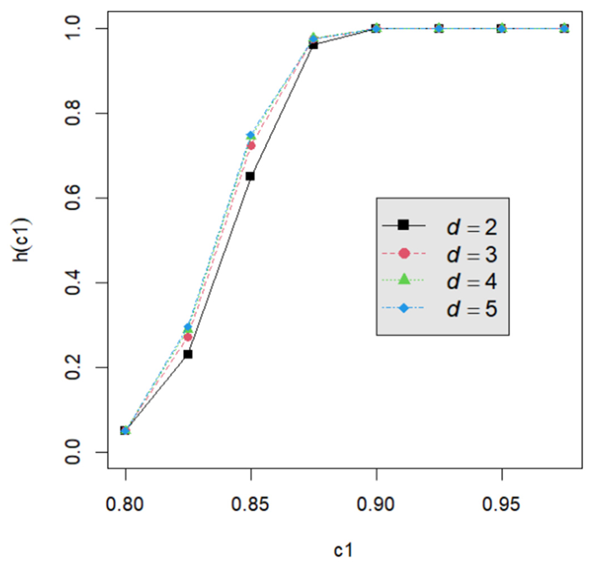
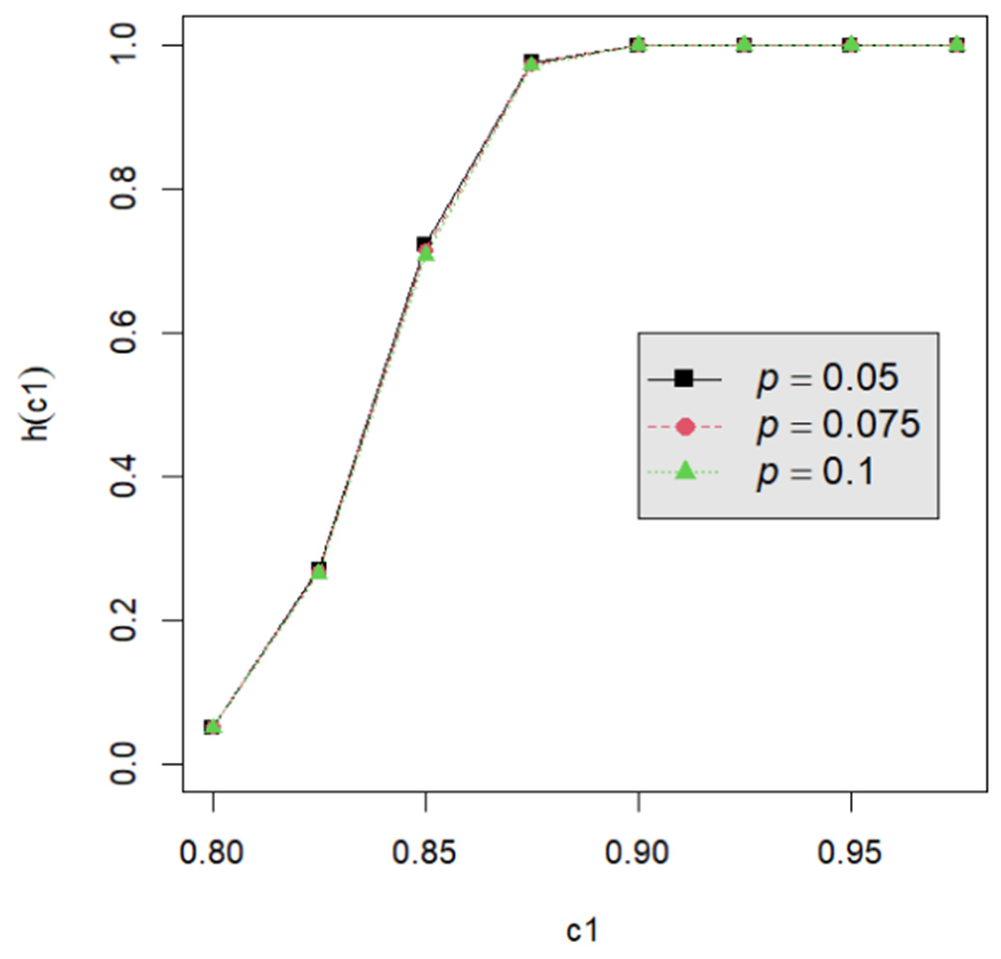
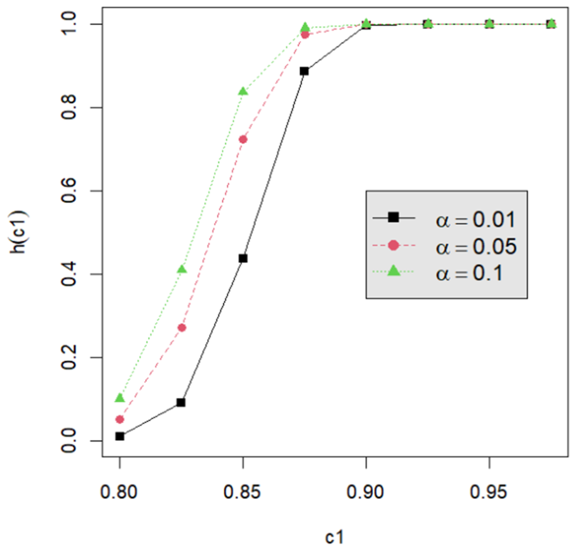
3.3. Test Power and Power Analysis
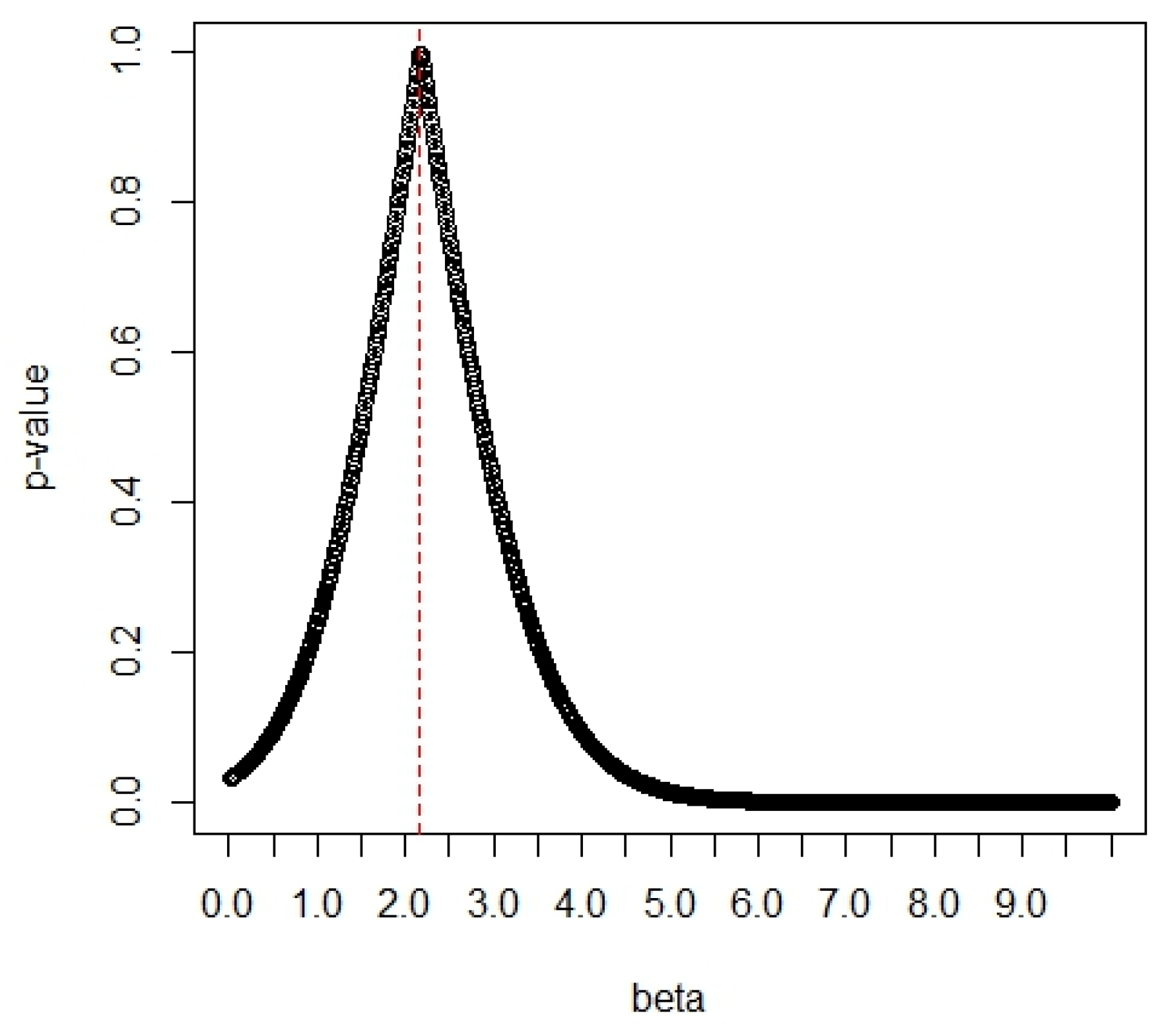
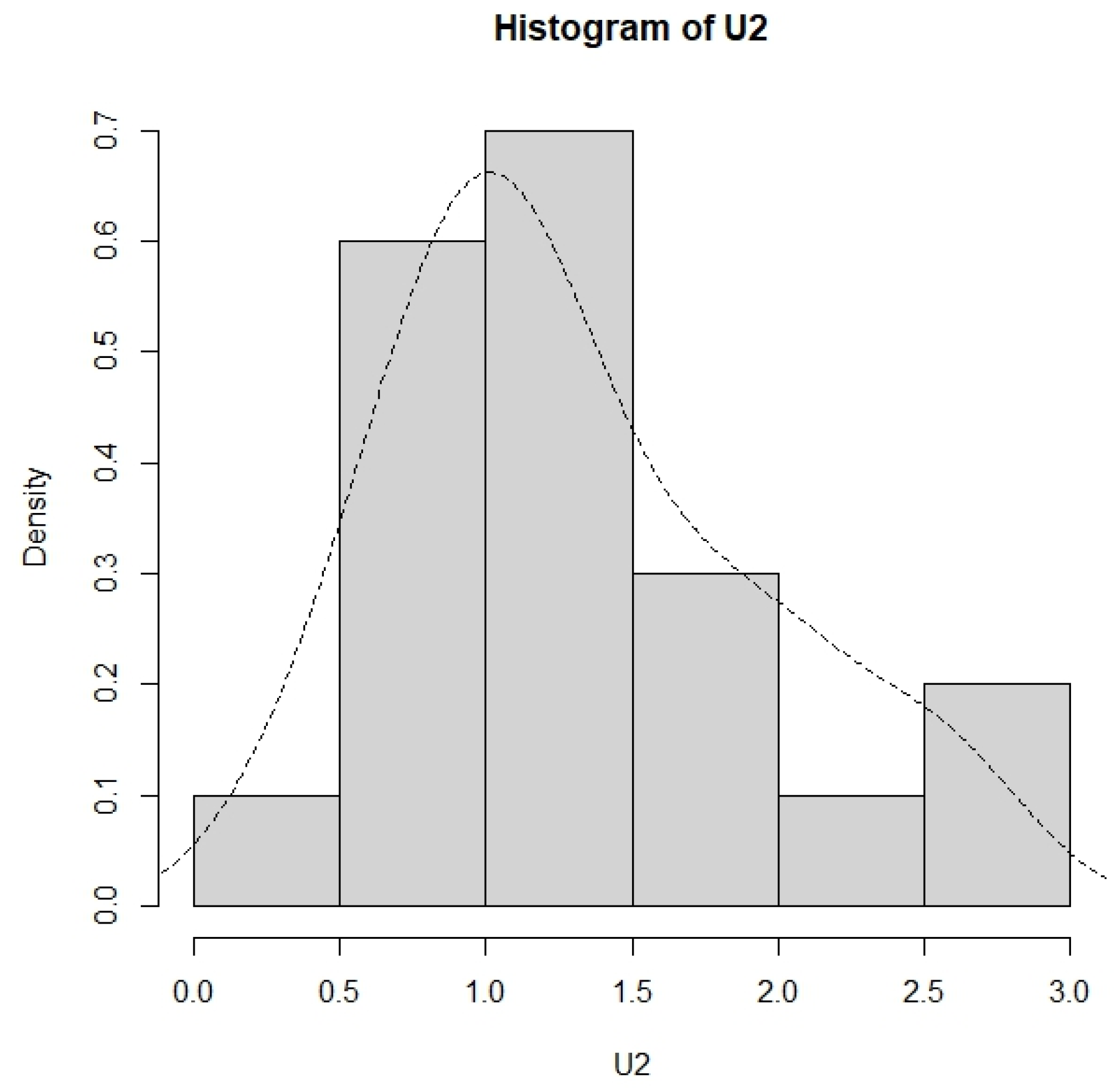
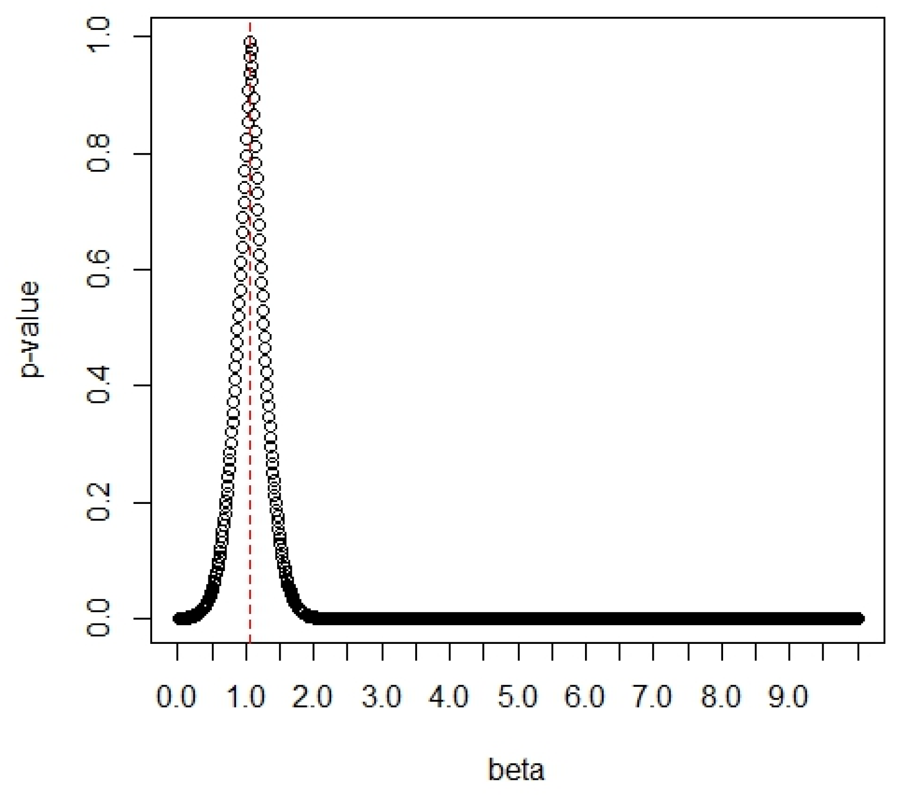
3.4. Example
| Algorithm 2: The implementation of the testing procedure for the overall lifetime performance index based on this numerical example. |
|
4. Conclusions
Author Contributions
Funding
Data Availability Statement
Conflicts of Interest
Appendix A

| d | ||||||
|---|---|---|---|---|---|---|
| Pr | CT | 2 | 3 | 4 | 5 | 6 |
| 0.6703 | 0.600 | 0.8000 | 0.8667 | 0.9000 | 0.9200 | 0.9333 |
| 0.6873 | 0.625 | 0.8125 | 0.8750 | 0.9063 | 0.9250 | 0.9375 |
| 0.7047 | 0.650 | 0.8250 | 0.8833 | 0.9125 | 0.9300 | 0.9417 |
| 0.7225 | 0.675 | 0.8375 | 0.8917 | 0.9188 | 0.9350 | 0.9458 |
| 0.7408 | 0.700 | 0.8500 | 0.9000 | 0.9250 | 0.9400 | 0.9500 |
| 0.7596 | 0.725 | 0.8625 | 0.9083 | 0.9313 | 0.9450 | 0.9542 |
| 0.7788 | 0.750 | 0.8750 | 0.9167 | 0.9375 | 0.9500 | 0.9583 |
| 0.7985 | 0.775 | 0.8875 | 0.9250 | 0.9438 | 0.9550 | 0.9625 |
| 0.8187 | 0.800 | 0.9000 | 0.9333 | 0.9500 | 0.9600 | 0.9667 |
| 0.8395 | 0.825 | 0.9125 | 0.9417 | 0.9563 | 0.9650 | 0.9708 |
| 0.8607 | 0.850 | 0.9250 | 0.9500 | 0.9625 | 0.9700 | 0.9750 |
| 0.8825 | 0.875 | 0.9375 | 0.9583 | 0.9688 | 0.9750 | 0.9792 |
| 0.9048 | 0.900 | 0.9500 | 0.9667 | 0.9750 | 0.9800 | 0.9833 |
| 0.9277 | 0.925 | 0.9625 | 0.9750 | 0.9813 | 0.9850 | 0.9875 |
| 0.9512 | 0.950 | 0.9750 | 0.9833 | 0.9875 | 0.9900 | 0.9917 |
| 0.9753 | 0.975 | 0.9875 | 0.9917 | 0.9938 | 0.9950 | 0.9958 |
| 1.0000 | 1.000 | 1.0000 | 1.0000 | 1.0000 | 1.0000 | 1.0000 |
| 0.800 | 0.825 | 0.850 | 0.875 | 0.900 | 0.925 | 0.950 | |||
|---|---|---|---|---|---|---|---|---|---|
| 5 | 40 | 0.050 | 0.0100 | 0.0686 | 0.3330 | 0.8136 | 0.9949 | 1.0000 | 1.0000 |
| 0.075 | 0.0100 | 0.0677 | 0.3268 | 0.8051 | 0.9941 | 1.0000 | 1.0000 | ||
| 0.100 | 0.0100 | 0.0668 | 0.3208 | 0.7967 | 0.9932 | 1.0000 | 1.0000 | ||
| 60 | 0.050 | 0.0100 | 0.1051 | 0.5308 | 0.9564 | 0.9999 | 1.0000 | 1.0000 | |
| 0.075 | 0.0100 | 0.1036 | 0.5224 | 0.9528 | 0.9999 | 1.0000 | 1.0000 | ||
| 0.100 | 0.0100 | 0.1020 | 0.5142 | 0.9491 | 0.9999 | 1.0000 | 1.0000 | ||
| 80 | 0.050 | 0.0100 | 0.1452 | 0.6903 | 0.9912 | 1.0000 | 1.0000 | 1.0000 | |
| 0.075 | 0.0100 | 0.1428 | 0.6817 | 0.9901 | 1.0000 | 1.0000 | 1.0000 | ||
| 0.100 | 0.0100 | 0.1406 | 0.6732 | 0.9890 | 1.0000 | 1.0000 | 1.0000 | ||
| 100 | 0.050 | 0.0100 | 0.1877 | 0.8048 | 0.9984 | 1.0000 | 1.0000 | 1.0000 | |
| 0.075 | 0.0100 | 0.1846 | 0.7972 | 0.9981 | 1.0000 | 1.0000 | 1.0000 | ||
| 0.100 | 0.0100 | 0.1817 | 0.7897 | 0.9978 | 1.0000 | 1.0000 | 1.0000 | ||
| 6 | 40 | 0.050 | 0.0100 | 0.0691 | 0.3342 | 0.8134 | 0.9947 | 1.0000 | 1.0000 |
| 0.075 | 0.0100 | 0.0679 | 0.3265 | 0.8029 | 0.9937 | 1.0000 | 1.0000 | ||
| 0.100 | 0.0100 | 0.0668 | 0.3192 | 0.7925 | 0.9925 | 1.0000 | 1.0000 | ||
| 60 | 0.050 | 0.0100 | 0.1058 | 0.5317 | 0.9561 | 0.9999 | 1.0000 | 1.0000 | |
| 0.075 | 0.0100 | 0.1038 | 0.5213 | 0.9515 | 0.9999 | 1.0000 | 1.0000 | ||
| 0.100 | 0.0100 | 0.1019 | 0.5112 | 0.9469 | 0.9998 | 1.0000 | 1.0000 | ||
| 80 | 0.050 | 0.0100 | 0.1459 | 0.6909 | 0.9911 | 1.0000 | 1.0000 | 1.0000 | |
| 0.075 | 0.0100 | 0.1430 | 0.6801 | 0.9897 | 1.0000 | 1.0000 | 1.0000 | ||
| 0.100 | 0.0100 | 0.1403 | 0.6697 | 0.9883 | 1.0000 | 1.0000 | 1.0000 | ||
| 100 | 0.050 | 0.0100 | 0.1886 | 0.8051 | 0.9984 | 1.0000 | 1.0000 | 1.0000 | |
| 0.075 | 0.0100 | 0.1848 | 0.7956 | 0.9980 | 1.0000 | 1.0000 | 1.0000 | ||
| 0.100 | 0.0100 | 0.1811 | 0.7863 | 0.9976 | 1.0000 | 1.0000 | 1.0000 | ||
| 7 | 40 | 0.050 | 0.0100 | 0.0692 | 0.3339 | 0.8118 | 0.9945 | 1.0000 | 1.0000 |
| 0.075 | 0.0100 | 0.0679 | 0.3248 | 0.7993 | 0.9932 | 1.0000 | 1.0000 | ||
| 0.100 | 0.0100 | 0.0666 | 0.3163 | 0.7870 | 0.9918 | 1.0000 | 1.0000 | ||
| 60 | 0.050 | 0.0100 | 0.1059 | 0.5310 | 0.9553 | 0.9999 | 1.0000 | 1.0000 | |
| 0.075 | 0.0100 | 0.1036 | 0.5186 | 0.9498 | 0.9999 | 1.0000 | 1.0000 | ||
| 0.100 | 0.0100 | 0.1014 | 0.5068 | 0.9442 | 0.9998 | 1.0000 | 1.0000 | ||
| 80 | 0.050 | 0.0100 | 0.1461 | 0.6899 | 0.9908 | 1.0000 | 1.0000 | 1.0000 | |
| 0.075 | 0.0100 | 0.1426 | 0.6771 | 0.9892 | 1.0000 | 1.0000 | 1.0000 | ||
| 0.100 | 0.0100 | 0.1394 | 0.6647 | 0.9873 | 1.0000 | 1.0000 | 1.0000 | ||
| 100 | 0.050 | 0.0100 | 0.1887 | 0.8040 | 0.9983 | 1.0000 | 1.0000 | 1.0000 | |
| 0.075 | 0.0100 | 0.1841 | 0.7927 | 0.9979 | 1.0000 | 1.0000 | 1.0000 | ||
| 0.100 | 0.0100 | 0.1798 | 0.7817 | 0.9974 | 1.0000 | 1.0000 | 1.0000 | ||
| 8 | 40 | 0.050 | 0.0100 | 0.0692 | 0.3329 | 0.8095 | 0.9942 | 1.0000 | 1.0000 |
| 0.075 | 0.0100 | 0.0676 | 0.3225 | 0.7950 | 0.9927 | 1.0000 | 1.0000 | ||
| 0.100 | 0.0100 | 0.0662 | 0.3128 | 0.7808 | 0.9909 | 1.0000 | 1.0000 | ||
| 60 | 0.050 | 0.0100 | 0.1058 | 0.5292 | 0.9542 | 0.9999 | 1.0000 | 1.0000 | |
| 0.075 | 0.0100 | 0.1031 | 0.5149 | 0.9477 | 0.9998 | 1.0000 | 1.0000 | ||
| 0.100 | 0.0100 | 0.1006 | 0.5015 | 0.9411 | 0.9998 | 1.0000 | 1.0000 | ||
| 80 | 0.050 | 0.0100 | 0.1458 | 0.6879 | 0.9905 | 1.0000 | 1.0000 | 1.0000 | |
| 0.075 | 0.0100 | 0.1419 | 0.6731 | 0.9885 | 1.0000 | 1.0000 | 1.0000 | ||
| 0.100 | 0.0100 | 0.1382 | 0.6590 | 0.9863 | 1.0000 | 1.0000 | 1.0000 | ||
| 100 | 0.050 | 0.0100 | 0.1884 | 0.8022 | 0.9982 | 1.0000 | 1.0000 | 1.0000 | |
| 0.075 | 0.0100 | 0.1831 | 0.7891 | 0.9977 | 1.0000 | 1.0000 | 1.0000 | ||
| 0.100 | 0.0100 | 0.1782 | 0.7764 | 0.9971 | 1.0000 | 1.0000 | 1.0000 | ||
| 0.800 | 0.825 | 0.850 | 0.875 | 0.900 | 0.925 | 0.950 | |||
|---|---|---|---|---|---|---|---|---|---|
| 5 | 40 | 0.050 | 0.0500 | 0.2307 | 0.6505 | 0.9619 | 0.9998 | 1.0000 | 1.0000 |
| 0.075 | 0.0500 | 0.2285 | 0.6439 | 0.9592 | 0.9998 | 1.0000 | 1.0000 | ||
| 0.100 | 0.0500 | 0.2263 | 0.6374 | 0.9565 | 0.9997 | 1.0000 | 1.0000 | ||
| 60 | 0.050 | 0.0500 | 0.3053 | 0.8093 | 0.9947 | 1.0000 | 1.0000 | 1.0000 | |
| 0.075 | 0.0500 | 0.3021 | 0.8033 | 0.9941 | 1.0000 | 1.0000 | 1.0000 | ||
| 0.100 | 0.0500 | 0.2991 | 0.7975 | 0.9935 | 1.0000 | 1.0000 | 1.0000 | ||
| 80 | 0.050 | 0.0500 | 0.3749 | 0.8992 | 0.9993 | 1.0000 | 1.0000 | 1.0000 | |
| 0.075 | 0.0500 | 0.3708 | 0.8948 | 0.9992 | 1.0000 | 1.0000 | 1.0000 | ||
| 0.100 | 0.0500 | 0.3670 | 0.8904 | 0.9991 | 1.0000 | 1.0000 | 1.0000 | ||
| 100 | 0.050 | 0.0500 | 0.4393 | 0.9478 | 0.9999 | 1.0000 | 1.0000 | 1.0000 | |
| 0.075 | 0.0500 | 0.4346 | 0.9449 | 0.9999 | 1.0000 | 1.0000 | 1.0000 | ||
| 0.100 | 0.0500 | 0.4301 | 0.9418 | 0.9999 | 1.0000 | 1.0000 | 1.0000 | ||
| 6 | 40 | 0.050 | 0.0500 | 0.2313 | 0.6506 | 0.9615 | 0.9998 | 1.0000 | 1.0000 |
| 0.075 | 0.0500 | 0.2285 | 0.6424 | 0.9581 | 0.9997 | 1.0000 | 1.0000 | ||
| 0.100 | 0.0500 | 0.2259 | 0.6345 | 0.9546 | 0.9997 | 1.0000 | 1.0000 | ||
| 60 | 0.050 | 0.0500 | 0.3060 | 0.8092 | 0.9946 | 1.0000 | 1.0000 | 1.0000 | |
| 0.075 | 0.0500 | 0.3020 | 0.8018 | 0.9939 | 1.0000 | 1.0000 | 1.0000 | ||
| 0.100 | 0.0500 | 0.2983 | 0.7945 | 0.9930 | 1.0000 | 1.0000 | 1.0000 | ||
| 80 | 0.050 | 0.0500 | 0.3756 | 0.8990 | 0.9993 | 1.0000 | 1.0000 | 1.0000 | |
| 0.075 | 0.0500 | 0.3706 | 0.8935 | 0.9992 | 1.0000 | 1.0000 | 1.0000 | ||
| 0.100 | 0.0500 | 0.3658 | 0.8880 | 0.9990 | 1.0000 | 1.0000 | 1.0000 | ||
| 100 | 0.050 | 0.0500 | 0.4400 | 0.9477 | 0.9999 | 1.0000 | 1.0000 | 1.0000 | |
| 0.075 | 0.0500 | 0.4342 | 0.9439 | 0.9999 | 1.0000 | 1.0000 | 1.0000 | ||
| 0.100 | 0.0500 | 0.4287 | 0.9402 | 0.9999 | 1.0000 | 1.0000 | 1.0000 | ||
| 7 | 40 | 0.050 | 0.0500 | 0.2313 | 0.6496 | 0.9608 | 0.9998 | 1.0000 | 1.0000 |
| 0.075 | 0.0500 | 0.2280 | 0.6399 | 0.9567 | 0.9997 | 1.0000 | 1.0000 | ||
| 0.100 | 0.0500 | 0.2249 | 0.6305 | 0.9524 | 0.9996 | 1.0000 | 1.0000 | ||
| 60 | 0.050 | 0.0500 | 0.3059 | 0.8081 | 0.9945 | 1.0000 | 1.0000 | 1.0000 | |
| 0.075 | 0.0500 | 0.3012 | 0.7993 | 0.9935 | 1.0000 | 1.0000 | 1.0000 | ||
| 0.100 | 0.0500 | 0.2968 | 0.7907 | 0.9925 | 1.0000 | 1.0000 | 1.0000 | ||
| 80 | 0.050 | 0.0500 | 0.3754 | 0.8982 | 0.9993 | 1.0000 | 1.0000 | 1.0000 | |
| 0.075 | 0.0500 | 0.3695 | 0.8916 | 0.9991 | 1.0000 | 1.0000 | 1.0000 | ||
| 0.100 | 0.0500 | 0.3639 | 0.8850 | 0.9989 | 1.0000 | 1.0000 | 1.0000 | ||
| 100 | 0.050 | 0.0500 | 0.4397 | 0.9471 | 0.9999 | 1.0000 | 1.0000 | 1.0000 | |
| 0.075 | 0.0500 | 0.4328 | 0.9426 | 0.9999 | 1.0000 | 1.0000 | 1.0000 | ||
| 0.100 | 0.0500 | 0.4263 | 0.9380 | 0.9998 | 1.0000 | 1.0000 | 1.0000 | ||
| 8 | 40 | 0.050 | 0.0500 | 0.2310 | 0.6479 | 0.9599 | 0.9998 | 1.0000 | 1.0000 |
| 0.075 | 0.0500 | 0.2272 | 0.6367 | 0.9550 | 0.9997 | 1.0000 | 1.0000 | ||
| 0.100 | 0.0500 | 0.2237 | 0.6261 | 0.9500 | 0.9995 | 1.0000 | 1.0000 | ||
| 60 | 0.050 | 0.0500 | 0.3054 | 0.8065 | 0.9942 | 1.0000 | 1.0000 | 1.0000 | |
| 0.075 | 0.0500 | 0.3000 | 0.7963 | 0.9931 | 1.0000 | 1.0000 | 1.0000 | ||
| 0.100 | 0.0500 | 0.2950 | 0.7864 | 0.9918 | 1.0000 | 1.0000 | 1.0000 | ||
| 80 | 0.050 | 0.0500 | 0.3747 | 0.8969 | 0.9992 | 1.0000 | 1.0000 | 1.0000 | |
| 0.075 | 0.0500 | 0.3679 | 0.8892 | 0.9990 | 1.0000 | 1.0000 | 1.0000 | ||
| 0.100 | 0.0500 | 0.3616 | 0.8816 | 0.9987 | 1.0000 | 1.0000 | 1.0000 | ||
| 100 | 0.050 | 0.0500 | 0.4389 | 0.9462 | 0.9999 | 1.0000 | 1.0000 | 1.0000 | |
| 0.075 | 0.0500 | 0.4309 | 0.9409 | 0.9999 | 1.0000 | 1.0000 | 1.0000 | ||
| 0.100 | 0.0500 | 0.4235 | 0.9356 | 0.9998 | 1.0000 | 1.0000 | 1.0000 | ||
| 0.800 | 0.825 | 0.850 | 0.875 | 0.900 | 0.925 | 0.950 | |||
|---|---|---|---|---|---|---|---|---|---|
| 5 | 40 | 0.050 | 0.1000 | 0.3670 | 0.7925 | 0.9873 | 1.0000 | 1.0000 | 1.0000 |
| 0.075 | 0.1000 | 0.3642 | 0.7872 | 0.9862 | 1.0000 | 1.0000 | 1.0000 | ||
| 0.100 | 0.1000 | 0.3614 | 0.7821 | 0.9850 | 1.0000 | 1.0000 | 1.0000 | ||
| 60 | 0.050 | 0.1000 | 0.4538 | 0.9019 | 0.9987 | 1.0000 | 1.0000 | 1.0000 | |
| 0.075 | 0.1000 | 0.4501 | 0.8981 | 0.9985 | 1.0000 | 1.0000 | 1.0000 | ||
| 0.100 | 0.1000 | 0.4465 | 0.8942 | 0.9983 | 1.0000 | 1.0000 | 1.0000 | ||
| 80 | 0.050 | 0.1000 | 0.5281 | 0.9541 | 0.9999 | 1.0000 | 1.0000 | 1.0000 | |
| 0.075 | 0.1000 | 0.5239 | 0.9516 | 0.9998 | 1.0000 | 1.0000 | 1.0000 | ||
| 0.100 | 0.1000 | 0.5197 | 0.9491 | 0.9998 | 1.0000 | 1.0000 | 1.0000 | ||
| 100 | 0.050 | 0.1000 | 0.5924 | 0.9786 | 1.0000 | 1.0000 | 1.0000 | 1.0000 | |
| 0.075 | 0.1000 | 0.5878 | 0.9771 | 1.0000 | 1.0000 | 1.0000 | 1.0000 | ||
| 0.100 | 0.1000 | 0.5832 | 0.9757 | 1.0000 | 1.0000 | 1.0000 | 1.0000 | ||
| 6 | 40 | 0.050 | 0.1000 | 0.3674 | 0.7921 | 0.9870 | 1.0000 | 1.0000 | 1.0000 |
| 0.075 | 0.1000 | 0.3639 | 0.7857 | 0.9856 | 1.0000 | 1.0000 | 1.0000 | ||
| 0.100 | 0.1000 | 0.3605 | 0.7793 | 0.9842 | 1.0000 | 1.0000 | 1.0000 | ||
| 60 | 0.050 | 0.1000 | 0.4542 | 0.9016 | 0.9986 | 1.0000 | 1.0000 | 1.0000 | |
| 0.075 | 0.1000 | 0.4497 | 0.8968 | 0.9984 | 1.0000 | 1.0000 | 1.0000 | ||
| 0.100 | 0.1000 | 0.4453 | 0.8921 | 0.9981 | 1.0000 | 1.0000 | 1.0000 | ||
| 80 | 0.050 | 0.1000 | 0.5286 | 0.9538 | 0.9999 | 1.0000 | 1.0000 | 1.0000 | |
| 0.075 | 0.1000 | 0.5233 | 0.9508 | 0.9998 | 1.0000 | 1.0000 | 1.0000 | ||
| 0.100 | 0.1000 | 0.5182 | 0.9477 | 0.9998 | 1.0000 | 1.0000 | 1.0000 | ||
| 100 | 0.050 | 0.1000 | 0.5928 | 0.9784 | 1.0000 | 1.0000 | 1.0000 | 1.0000 | |
| 0.075 | 0.1000 | 0.5871 | 0.9766 | 1.0000 | 1.0000 | 1.0000 | 1.0000 | ||
| 0.100 | 0.1000 | 0.5815 | 0.9747 | 1.0000 | 1.0000 | 1.0000 | 1.0000 | ||
| 7 | 40 | 0.050 | 0.1000 | 0.3673 | 0.7911 | 0.9867 | 1.0000 | 1.0000 | 1.0000 |
| 0.075 | 0.1000 | 0.3631 | 0.7833 | 0.9850 | 1.0000 | 1.0000 | 1.0000 | ||
| 0.100 | 0.1000 | 0.3591 | 0.7759 | 0.9832 | 0.9999 | 1.0000 | 1.0000 | ||
| 60 | 0.050 | 0.1000 | 0.4539 | 0.9007 | 0.9986 | 1.0000 | 1.0000 | 1.0000 | |
| 0.075 | 0.1000 | 0.4485 | 0.8950 | 0.9983 | 1.0000 | 1.0000 | 1.0000 | ||
| 0.100 | 0.1000 | 0.4434 | 0.8894 | 0.9980 | 1.0000 | 1.0000 | 1.0000 | ||
| 80 | 0.050 | 0.1000 | 0.5282 | 0.9532 | 0.9999 | 1.0000 | 1.0000 | 1.0000 | |
| 0.075 | 0.1000 | 0.5219 | 0.9496 | 0.9998 | 1.0000 | 1.0000 | 1.0000 | ||
| 0.100 | 0.1000 | 0.5159 | 0.9459 | 0.9998 | 1.0000 | 1.0000 | 1.0000 | ||
| 100 | 0.050 | 0.1000 | 0.5924 | 0.9781 | 1.0000 | 1.0000 | 1.0000 | 1.0000 | |
| 0.075 | 0.1000 | 0.5855 | 0.9759 | 1.0000 | 1.0000 | 1.0000 | 1.0000 | ||
| 0.100 | 0.1000 | 0.5790 | 0.9736 | 1.0000 | 1.0000 | 1.0000 | 1.0000 | ||
| 8 | 40 | 0.050 | 0.1000 | 0.3668 | 0.7895 | 0.9863 | 1.0000 | 1.0000 | 1.0000 |
| 0.075 | 0.1000 | 0.3619 | 0.7806 | 0.9843 | 1.0000 | 1.0000 | 1.0000 | ||
| 0.100 | 0.1000 | 0.3574 | 0.7720 | 0.9821 | 0.9999 | 1.0000 | 1.0000 | ||
| 60 | 0.050 | 0.1000 | 0.4532 | 0.8995 | 0.9985 | 1.0000 | 1.0000 | 1.0000 | |
| 0.075 | 0.1000 | 0.4470 | 0.8929 | 0.9982 | 1.0000 | 1.0000 | 1.0000 | ||
| 0.100 | 0.1000 | 0.4411 | 0.8864 | 0.9978 | 1.0000 | 1.0000 | 1.0000 | ||
| 80 | 0.050 | 0.1000 | 0.5273 | 0.9525 | 0.9998 | 1.0000 | 1.0000 | 1.0000 | |
| 0.075 | 0.1000 | 0.5201 | 0.9482 | 0.9998 | 1.0000 | 1.0000 | 1.0000 | ||
| 0.100 | 0.1000 | 0.5132 | 0.9438 | 0.9997 | 1.0000 | 1.0000 | 1.0000 | ||
| 100 | 0.050 | 0.1000 | 0.5914 | 0.9776 | 1.0000 | 1.0000 | 1.0000 | 1.0000 | |
| 0.075 | 0.1000 | 0.5835 | 0.9750 | 1.0000 | 1.0000 | 1.0000 | 1.0000 | ||
| 0.100 | 0.1000 | 0.5760 | 0.9724 | 1.0000 | 1.0000 | 1.0000 | 1.0000 | ||
| 0.800 | 0.825 | 0.850 | 0.875 | 0.900 | 0.925 | 0.950 | |||
|---|---|---|---|---|---|---|---|---|---|
| 5 | 40 | 0.050 | 0.0100 | 0.0916 | 0.4380 | 0.8880 | 0.9978 | 1.0000 | 1.0000 |
| 0.075 | 0.0100 | 0.0899 | 0.4288 | 0.8805 | 0.9973 | 1.0000 | 1.0000 | ||
| 0.100 | 0.0100 | 0.0883 | 0.4200 | 0.8729 | 0.9968 | 1.0000 | 1.0000 | ||
| 60 | 0.050 | 0.0100 | 0.1390 | 0.6377 | 0.9764 | 1.0000 | 1.0000 | 1.0000 | |
| 0.075 | 0.0100 | 0.1362 | 0.6272 | 0.9738 | 0.9999 | 1.0000 | 1.0000 | ||
| 0.100 | 0.0100 | 0.1335 | 0.6169 | 0.9711 | 0.9999 | 1.0000 | 1.0000 | ||
| 80 | 0.050 | 0.0100 | 0.1895 | 0.7780 | 0.9954 | 1.0000 | 1.0000 | 1.0000 | |
| 0.075 | 0.0100 | 0.1855 | 0.7685 | 0.9947 | 1.0000 | 1.0000 | 1.0000 | ||
| 0.100 | 0.0100 | 0.1817 | 0.7591 | 0.9939 | 1.0000 | 1.0000 | 1.0000 | ||
| 100 | 0.050 | 0.0100 | 0.2416 | 0.8682 | 0.9991 | 1.0000 | 1.0000 | 1.0000 | |
| 0.075 | 0.0100 | 0.2365 | 0.8607 | 0.9990 | 1.0000 | 1.0000 | 1.0000 | ||
| 0.100 | 0.0100 | 0.2316 | 0.8532 | 0.9988 | 1.0000 | 1.0000 | 1.0000 | ||
| 6 | 40 | 0.050 | 0.0100 | 0.0911 | 0.4349 | 0.8851 | 0.9976 | 1.0000 | 1.0000 |
| 0.075 | 0.0100 | 0.0891 | 0.4236 | 0.8756 | 0.9970 | 1.0000 | 1.0000 | ||
| 0.100 | 0.0100 | 0.0871 | 0.4128 | 0.8661 | 0.9963 | 1.0000 | 1.0000 | ||
| 60 | 0.050 | 0.0100 | 0.1382 | 0.6340 | 0.9754 | 1.0000 | 1.0000 | 1.0000 | |
| 0.075 | 0.0100 | 0.1347 | 0.6209 | 0.9720 | 0.9999 | 1.0000 | 1.0000 | ||
| 0.100 | 0.0100 | 0.1315 | 0.6083 | 0.9685 | 0.9999 | 1.0000 | 1.0000 | ||
| 80 | 0.050 | 0.0100 | 0.1883 | 0.7746 | 0.9951 | 1.0000 | 1.0000 | 1.0000 | |
| 0.075 | 0.0100 | 0.1834 | 0.7628 | 0.9941 | 1.0000 | 1.0000 | 1.0000 | ||
| 0.100 | 0.0100 | 0.1788 | 0.7511 | 0.9931 | 1.0000 | 1.0000 | 1.0000 | ||
| 100 | 0.050 | 0.0100 | 0.2400 | 0.8655 | 0.9991 | 1.0000 | 1.0000 | 1.0000 | |
| 0.075 | 0.0100 | 0.2338 | 0.8561 | 0.9988 | 1.0000 | 1.0000 | 1.0000 | ||
| 0.100 | 0.0100 | 0.2279 | 0.8467 | 0.9985 | 1.0000 | 1.0000 | 1.0000 | ||
| 7 | 40 | 0.050 | 0.0100 | 0.0906 | 0.4313 | 0.8818 | 0.9974 | 1.0000 | 1.0000 |
| 0.075 | 0.0100 | 0.0881 | 0.4179 | 0.8704 | 0.9966 | 1.0000 | 1.0000 | ||
| 0.100 | 0.0100 | 0.0858 | 0.4053 | 0.8589 | 0.9957 | 1.0000 | 1.0000 | ||
| 60 | 0.050 | 0.0100 | 0.1372 | 0.6297 | 0.9742 | 0.9999 | 1.0000 | 1.0000 | |
| 0.075 | 0.0100 | 0.1331 | 0.6142 | 0.9701 | 0.9999 | 1.0000 | 1.0000 | ||
| 0.100 | 0.0100 | 0.1293 | 0.5994 | 0.9656 | 0.9999 | 1.0000 | 1.0000 | ||
| 80 | 0.050 | 0.0100 | 0.1868 | 0.7707 | 0.9948 | 1.0000 | 1.0000 | 1.0000 | |
| 0.075 | 0.0100 | 0.1811 | 0.7566 | 0.9936 | 1.0000 | 1.0000 | 1.0000 | ||
| 0.100 | 0.0100 | 0.1758 | 0.7427 | 0.9922 | 1.0000 | 1.0000 | 1.0000 | ||
| 100 | 0.050 | 0.0100 | 0.2381 | 0.8624 | 0.9990 | 1.0000 | 1.0000 | 1.0000 | |
| 0.075 | 0.0100 | 0.2308 | 0.8511 | 0.9987 | 1.0000 | 1.0000 | 1.0000 | ||
| 0.100 | 0.0100 | 0.2239 | 0.8398 | 0.9983 | 1.0000 | 1.0000 | 1.0000 | ||
| 8 | 40 | 0.050 | 0.0100 | 0.0899 | 0.4274 | 0.8784 | 0.9971 | 1.0000 | 1.0000 |
| 0.075 | 0.0100 | 0.0871 | 0.4121 | 0.8650 | 0.9962 | 1.0000 | 1.0000 | ||
| 0.100 | 0.0100 | 0.0845 | 0.3979 | 0.8515 | 0.9951 | 1.0000 | 1.0000 | ||
| 60 | 0.050 | 0.0100 | 0.1361 | 0.6252 | 0.9730 | 0.9999 | 1.0000 | 1.0000 | |
| 0.075 | 0.0100 | 0.1314 | 0.6073 | 0.9680 | 0.9999 | 1.0000 | 1.0000 | ||
| 0.100 | 0.0100 | 0.1272 | 0.5904 | 0.9626 | 0.9999 | 1.0000 | 1.0000 | ||
| 80 | 0.050 | 0.0100 | 0.1852 | 0.7665 | 0.9944 | 1.0000 | 1.0000 | 1.0000 | |
| 0.075 | 0.0100 | 0.1787 | 0.7501 | 0.9929 | 1.0000 | 1.0000 | 1.0000 | ||
| 0.100 | 0.0100 | 0.1727 | 0.7341 | 0.9912 | 1.0000 | 1.0000 | 1.0000 | ||
| 100 | 0.050 | 0.0100 | 0.2361 | 0.8591 | 0.9989 | 1.0000 | 1.0000 | 1.0000 | |
| 0.075 | 0.0100 | 0.2277 | 0.8458 | 0.9985 | 1.0000 | 1.0000 | 1.0000 | ||
| 0.100 | 0.0100 | 0.2200 | 0.8326 | 0.9980 | 1.0000 | 1.0000 | 1.0000 | ||
| 0.800 | 0.825 | 0.850 | 0.875 | 0.900 | 0.925 | 0.950 | |||
|---|---|---|---|---|---|---|---|---|---|
| 5 | 40 | 0.050 | 0.0500 | 0.2711 | 0.7230 | 0.9760 | 0.9999 | 1.0000 | 1.0000 |
| 0.075 | 0.0500 | 0.2677 | 0.7153 | 0.9738 | 0.9998 | 1.0000 | 1.0000 | ||
| 0.100 | 0.0500 | 0.2643 | 0.7076 | 0.9715 | 0.9998 | 1.0000 | 1.0000 | ||
| 60 | 0.050 | 0.0500 | 0.3544 | 0.8579 | 0.9966 | 1.0000 | 1.0000 | 1.0000 | |
| 0.075 | 0.0500 | 0.3497 | 0.8517 | 0.9961 | 1.0000 | 1.0000 | 1.0000 | ||
| 0.100 | 0.0500 | 0.3451 | 0.8455 | 0.9956 | 1.0000 | 1.0000 | 1.0000 | ||
| 80 | 0.050 | 0.0500 | 0.4296 | 0.9279 | 0.9995 | 1.0000 | 1.0000 | 1.0000 | |
| 0.075 | 0.0500 | 0.4239 | 0.9236 | 0.9994 | 1.0000 | 1.0000 | 1.0000 | ||
| 0.100 | 0.0500 | 0.4184 | 0.9193 | 0.9993 | 1.0000 | 1.0000 | 1.0000 | ||
| 100 | 0.050 | 0.0500 | 0.4973 | 0.9636 | 0.9999 | 1.0000 | 1.0000 | 1.0000 | |
| 0.075 | 0.0500 | 0.4909 | 0.9608 | 0.9999 | 1.0000 | 1.0000 | 1.0000 | ||
| 0.100 | 0.0500 | 0.4847 | 0.9580 | 0.9999 | 1.0000 | 1.0000 | 1.0000 | ||
| 6 | 40 | 0.050 | 0.0500 | 0.2700 | 0.7201 | 0.9751 | 0.9999 | 1.0000 | 1.0000 |
| 0.075 | 0.0500 | 0.2658 | 0.7104 | 0.9723 | 0.9998 | 1.0000 | 1.0000 | ||
| 0.100 | 0.0500 | 0.2617 | 0.7010 | 0.9693 | 0.9998 | 1.0000 | 1.0000 | ||
| 60 | 0.050 | 0.0500 | 0.3529 | 0.8555 | 0.9964 | 1.0000 | 1.0000 | 1.0000 | |
| 0.075 | 0.0500 | 0.3471 | 0.8477 | 0.9958 | 1.0000 | 1.0000 | 1.0000 | ||
| 0.100 | 0.0500 | 0.3415 | 0.8400 | 0.9951 | 1.0000 | 1.0000 | 1.0000 | ||
| 80 | 0.050 | 0.0500 | 0.4277 | 0.9263 | 0.9995 | 1.0000 | 1.0000 | 1.0000 | |
| 0.075 | 0.0500 | 0.4207 | 0.9208 | 0.9994 | 1.0000 | 1.0000 | 1.0000 | ||
| 0.100 | 0.0500 | 0.4140 | 0.9154 | 0.9992 | 1.0000 | 1.0000 | 1.0000 | ||
| 100 | 0.050 | 0.0500 | 0.4952 | 0.9625 | 0.9999 | 1.0000 | 1.0000 | 1.0000 | |
| 0.075 | 0.0500 | 0.4872 | 0.9590 | 0.9999 | 1.0000 | 1.0000 | 1.0000 | ||
| 0.100 | 0.0500 | 0.4796 | 0.9554 | 0.9999 | 1.0000 | 1.0000 | 1.0000 | ||
| 7 | 40 | 0.050 | 0.0500 | 0.2687 | 0.7168 | 0.9741 | 0.9998 | 1.0000 | 1.0000 |
| 0.075 | 0.0500 | 0.2637 | 0.7053 | 0.9706 | 0.9998 | 1.0000 | 1.0000 | ||
| 0.100 | 0.0500 | 0.2590 | 0.6942 | 0.9670 | 0.9997 | 1.0000 | 1.0000 | ||
| 60 | 0.050 | 0.0500 | 0.3511 | 0.8529 | 0.9962 | 1.0000 | 1.0000 | 1.0000 | |
| 0.075 | 0.0500 | 0.3442 | 0.8435 | 0.9954 | 1.0000 | 1.0000 | 1.0000 | ||
| 0.100 | 0.0500 | 0.3377 | 0.8343 | 0.9945 | 1.0000 | 1.0000 | 1.0000 | ||
| 80 | 0.050 | 0.0500 | 0.4255 | 0.9244 | 0.9994 | 1.0000 | 1.0000 | 1.0000 | |
| 0.075 | 0.0500 | 0.4172 | 0.9179 | 0.9993 | 1.0000 | 1.0000 | 1.0000 | ||
| 0.100 | 0.0500 | 0.4094 | 0.9112 | 0.9991 | 1.0000 | 1.0000 | 1.0000 | ||
| 100 | 0.050 | 0.0500 | 0.4926 | 0.9613 | 0.9999 | 1.0000 | 1.0000 | 1.0000 | |
| 0.075 | 0.0500 | 0.4833 | 0.9571 | 0.9999 | 1.0000 | 1.0000 | 1.0000 | ||
| 0.100 | 0.0500 | 0.4744 | 0.9527 | 0.9999 | 1.0000 | 1.0000 | 1.0000 | ||
| 8 | 40 | 0.050 | 0.0500 | 0.2673 | 0.7133 | 0.9730 | 0.9998 | 1.0000 | 1.0000 |
| 0.075 | 0.0500 | 0.2615 | 0.7001 | 0.9689 | 0.9997 | 1.0000 | 1.0000 | ||
| 0.100 | 0.0500 | 0.2562 | 0.6874 | 0.9645 | 0.9996 | 1.0000 | 1.0000 | ||
| 60 | 0.050 | 0.0500 | 0.3491 | 0.8500 | 0.9960 | 1.0000 | 1.0000 | 1.0000 | |
| 0.075 | 0.0500 | 0.3412 | 0.8392 | 0.9950 | 1.0000 | 1.0000 | 1.0000 | ||
| 0.100 | 0.0500 | 0.3339 | 0.8285 | 0.9939 | 1.0000 | 1.0000 | 1.0000 | ||
| 80 | 0.050 | 0.0500 | 0.4231 | 0.9224 | 0.9994 | 1.0000 | 1.0000 | 1.0000 | |
| 0.075 | 0.0500 | 0.4136 | 0.9147 | 0.9992 | 1.0000 | 1.0000 | 1.0000 | ||
| 0.100 | 0.0500 | 0.4047 | 0.9070 | 0.9989 | 1.0000 | 1.0000 | 1.0000 | ||
| 100 | 0.050 | 0.0500 | 0.4899 | 0.9601 | 0.9999 | 1.0000 | 1.0000 | 1.0000 | |
| 0.075 | 0.0500 | 0.4792 | 0.9550 | 0.9999 | 1.0000 | 1.0000 | 1.0000 | ||
| 0.100 | 0.0500 | 0.4691 | 0.9498 | 0.9998 | 1.0000 | 1.0000 | 1.0000 | ||
| 0.800 | 0.825 | 0.850 | 0.875 | 0.900 | 0.925 | 0.950 | |||
|---|---|---|---|---|---|---|---|---|---|
| 5 | 40 | 0.050 | 0.1000 | 0.4094 | 0.8368 | 0.9913 | 1.0000 | 1.0000 | 1.0000 |
| 0.075 | 0.1000 | 0.4053 | 0.8311 | 0.9903 | 1.0000 | 1.0000 | 1.0000 | ||
| 0.100 | 0.1000 | 0.4014 | 0.8254 | 0.9893 | 1.0000 | 1.0000 | 1.0000 | ||
| 60 | 0.050 | 0.1000 | 0.5003 | 0.9258 | 0.9990 | 1.0000 | 1.0000 | 1.0000 | |
| 0.075 | 0.1000 | 0.4953 | 0.9220 | 0.9989 | 1.0000 | 1.0000 | 1.0000 | ||
| 0.100 | 0.1000 | 0.4904 | 0.9181 | 0.9987 | 1.0000 | 1.0000 | 1.0000 | ||
| 80 | 0.050 | 0.1000 | 0.5760 | 0.9659 | 0.9999 | 1.0000 | 1.0000 | 1.0000 | |
| 0.075 | 0.1000 | 0.5704 | 0.9635 | 0.9999 | 1.0000 | 1.0000 | 1.0000 | ||
| 0.100 | 0.1000 | 0.5649 | 0.9611 | 0.9998 | 1.0000 | 1.0000 | 1.0000 | ||
| 100 | 0.050 | 0.1000 | 0.6397 | 0.9842 | 1.0000 | 1.0000 | 1.0000 | 1.0000 | |
| 0.075 | 0.1000 | 0.6337 | 0.9828 | 1.0000 | 1.0000 | 1.0000 | 1.0000 | ||
| 0.100 | 0.1000 | 0.6279 | 0.9814 | 1.0000 | 1.0000 | 1.0000 | 1.0000 | ||
| 6 | 40 | 0.050 | 0.1000 | 0.4080 | 0.8345 | 0.9909 | 1.0000 | 1.0000 | 1.0000 |
| 0.075 | 0.1000 | 0.4030 | 0.8274 | 0.9896 | 1.0000 | 1.0000 | 1.0000 | ||
| 0.100 | 0.1000 | 0.3982 | 0.8204 | 0.9884 | 1.0000 | 1.0000 | 1.0000 | ||
| 60 | 0.050 | 0.1000 | 0.4986 | 0.9243 | 0.9989 | 1.0000 | 1.0000 | 1.0000 | |
| 0.075 | 0.1000 | 0.4924 | 0.9194 | 0.9987 | 1.0000 | 1.0000 | 1.0000 | ||
| 0.100 | 0.1000 | 0.4864 | 0.9145 | 0.9985 | 1.0000 | 1.0000 | 1.0000 | ||
| 80 | 0.050 | 0.1000 | 0.5741 | 0.9649 | 0.9999 | 1.0000 | 1.0000 | 1.0000 | |
| 0.075 | 0.1000 | 0.5671 | 0.9620 | 0.9998 | 1.0000 | 1.0000 | 1.0000 | ||
| 0.100 | 0.1000 | 0.5604 | 0.9589 | 0.9998 | 1.0000 | 1.0000 | 1.0000 | ||
| 100 | 0.050 | 0.1000 | 0.6376 | 0.9836 | 1.0000 | 1.0000 | 1.0000 | 1.0000 | |
| 0.075 | 0.1000 | 0.6302 | 0.9819 | 1.0000 | 1.0000 | 1.0000 | 1.0000 | ||
| 0.100 | 0.1000 | 0.6231 | 0.9800 | 1.0000 | 1.0000 | 1.0000 | 1.0000 | ||
| 7 | 40 | 0.050 | 0.1000 | 0.4064 | 0.8320 | 0.9904 | 1.0000 | 1.0000 | 1.0000 |
| 0.075 | 0.1000 | 0.4004 | 0.8235 | 0.9889 | 1.0000 | 1.0000 | 1.0000 | ||
| 0.100 | 0.1000 | 0.3949 | 0.8152 | 0.9873 | 0.9999 | 1.0000 | 1.0000 | ||
| 60 | 0.050 | 0.1000 | 0.4966 | 0.9226 | 0.9989 | 1.0000 | 1.0000 | 1.0000 | |
| 0.075 | 0.1000 | 0.4892 | 0.9167 | 0.9986 | 1.0000 | 1.0000 | 1.0000 | ||
| 0.100 | 0.1000 | 0.4822 | 0.9108 | 0.9983 | 1.0000 | 1.0000 | 1.0000 | ||
| 80 | 0.050 | 0.1000 | 0.5718 | 0.9639 | 0.9999 | 1.0000 | 1.0000 | 1.0000 | |
| 0.075 | 0.1000 | 0.5635 | 0.9603 | 0.9998 | 1.0000 | 1.0000 | 1.0000 | ||
| 0.100 | 0.1000 | 0.5557 | 0.9565 | 0.9998 | 1.0000 | 1.0000 | 1.0000 | ||
| 100 | 0.050 | 0.1000 | 0.6352 | 0.9830 | 1.0000 | 1.0000 | 1.0000 | 1.0000 | |
| 0.075 | 0.1000 | 0.6264 | 0.9809 | 1.0000 | 1.0000 | 1.0000 | 1.0000 | ||
| 0.100 | 0.1000 | 0.6181 | 0.9786 | 1.0000 | 1.0000 | 1.0000 | 1.0000 | ||
| 8 | 40 | 0.050 | 0.1000 | 0.4046 | 0.8294 | 0.9900 | 1.0000 | 1.0000 | 1.0000 |
| 0.075 | 0.1000 | 0.3979 | 0.8195 | 0.9881 | 1.0000 | 1.0000 | 1.0000 | ||
| 0.100 | 0.1000 | 0.3915 | 0.8100 | 0.9862 | 0.9999 | 1.0000 | 1.0000 | ||
| 60 | 0.050 | 0.1000 | 0.4944 | 0.9208 | 0.9988 | 1.0000 | 1.0000 | 1.0000 | |
| 0.075 | 0.1000 | 0.4860 | 0.9139 | 0.9984 | 1.0000 | 1.0000 | 1.0000 | ||
| 0.100 | 0.1000 | 0.4781 | 0.9071 | 0.9981 | 1.0000 | 1.0000 | 1.0000 | ||
| 80 | 0.050 | 0.1000 | 0.5694 | 0.9628 | 0.9999 | 1.0000 | 1.0000 | 1.0000 | |
| 0.075 | 0.1000 | 0.5599 | 0.9585 | 0.9998 | 1.0000 | 1.0000 | 1.0000 | ||
| 0.100 | 0.1000 | 0.5509 | 0.9541 | 0.9997 | 1.0000 | 1.0000 | 1.0000 | ||
| 100 | 0.050 | 0.1000 | 0.6326 | 0.9824 | 1.0000 | 1.0000 | 1.0000 | 1.0000 | |
| 0.075 | 0.1000 | 0.6225 | 0.9798 | 1.0000 | 1.0000 | 1.0000 | 1.0000 | ||
| 0.100 | 0.1000 | 0.6130 | 0.9771 | 1.0000 | 1.0000 | 1.0000 | 1.0000 | ||
| 0.800 | 0.825 | 0.850 | 0.875 | 0.900 | 0.925 | 0.950 | |||
|---|---|---|---|---|---|---|---|---|---|
| 5 | 40 | 0.050 | 0.0100 | 0.1037 | 0.4806 | 0.9049 | 0.9979 | 1.0000 | 1.0000 |
| 0.075 | 0.0100 | 0.1015 | 0.4702 | 0.8979 | 0.9975 | 1.0000 | 1.0000 | ||
| 0.100 | 0.0100 | 0.0994 | 0.4601 | 0.8907 | 0.9970 | 1.0000 | 1.0000 | ||
| 60 | 0.050 | 0.0100 | 0.1555 | 0.6721 | 0.9790 | 0.9999 | 1.0000 | 1.0000 | |
| 0.075 | 0.0100 | 0.1520 | 0.6609 | 0.9765 | 0.9999 | 1.0000 | 1.0000 | ||
| 0.100 | 0.0100 | 0.1486 | 0.6499 | 0.9739 | 0.9999 | 1.0000 | 1.0000 | ||
| 80 | 0.050 | 0.0100 | 0.2097 | 0.8008 | 0.9955 | 1.0000 | 1.0000 | 1.0000 | |
| 0.075 | 0.0100 | 0.2048 | 0.7911 | 0.9948 | 1.0000 | 1.0000 | 1.0000 | ||
| 0.100 | 0.0100 | 0.2002 | 0.7814 | 0.9940 | 1.0000 | 1.0000 | 1.0000 | ||
| 100 | 0.050 | 0.0100 | 0.2647 | 0.8816 | 0.9990 | 1.0000 | 1.0000 | 1.0000 | |
| 0.075 | 0.0100 | 0.2585 | 0.8740 | 0.9989 | 1.0000 | 1.0000 | 1.0000 | ||
| 0.100 | 0.0100 | 0.2527 | 0.8664 | 0.9986 | 1.0000 | 1.0000 | 1.0000 | ||
| 6 | 40 | 0.050 | 0.0100 | 0.1028 | 0.4760 | 0.9017 | 0.9977 | 1.0000 | 1.0000 |
| 0.075 | 0.0100 | 0.1001 | 0.4632 | 0.8927 | 0.9972 | 1.0000 | 1.0000 | ||
| 0.100 | 0.0100 | 0.0976 | 0.4509 | 0.8835 | 0.9965 | 1.0000 | 1.0000 | ||
| 60 | 0.050 | 0.0100 | 0.1540 | 0.6671 | 0.9779 | 0.9999 | 1.0000 | 1.0000 | |
| 0.075 | 0.0100 | 0.1497 | 0.6532 | 0.9747 | 0.9999 | 1.0000 | 1.0000 | ||
| 0.100 | 0.0100 | 0.1456 | 0.6397 | 0.9712 | 0.9999 | 1.0000 | 1.0000 | ||
| 80 | 0.050 | 0.0100 | 0.2076 | 0.7965 | 0.9952 | 1.0000 | 1.0000 | 1.0000 | |
| 0.075 | 0.0100 | 0.2016 | 0.7843 | 0.9942 | 1.0000 | 1.0000 | 1.0000 | ||
| 0.100 | 0.0100 | 0.1960 | 0.7722 | 0.9931 | 1.0000 | 1.0000 | 1.0000 | ||
| 100 | 0.050 | 0.0100 | 0.2620 | 0.8782 | 0.9990 | 1.0000 | 1.0000 | 1.0000 | |
| 0.075 | 0.0100 | 0.2545 | 0.8687 | 0.9987 | 1.0000 | 1.0000 | 1.0000 | ||
| 0.100 | 0.0100 | 0.2475 | 0.8591 | 0.9984 | 1.0000 | 1.0000 | 1.0000 | ||
| 7 | 40 | 0.050 | 0.0100 | 0.1018 | 0.4711 | 0.8983 | 0.9975 | 1.0000 | 1.0000 |
| 0.075 | 0.0100 | 0.0987 | 0.4560 | 0.8874 | 0.9968 | 1.0000 | 1.0000 | ||
| 0.100 | 0.0100 | 0.0957 | 0.4418 | 0.8762 | 0.9959 | 1.0000 | 1.0000 | ||
| 60 | 0.050 | 0.0100 | 0.1524 | 0.6619 | 0.9767 | 0.9999 | 1.0000 | 1.0000 | |
| 0.075 | 0.0100 | 0.1474 | 0.6453 | 0.9726 | 0.9999 | 1.0000 | 1.0000 | ||
| 0.100 | 0.0100 | 0.1427 | 0.6294 | 0.9683 | 0.9998 | 1.0000 | 1.0000 | ||
| 80 | 0.050 | 0.0100 | 0.2054 | 0.7919 | 0.9948 | 1.0000 | 1.0000 | 1.0000 | |
| 0.075 | 0.0100 | 0.1984 | 0.7773 | 0.9936 | 1.0000 | 1.0000 | 1.0000 | ||
| 0.100 | 0.0100 | 0.1920 | 0.7629 | 0.9921 | 1.0000 | 1.0000 | 1.0000 | ||
| 100 | 0.050 | 0.0100 | 0.2593 | 0.8746 | 0.9989 | 1.0000 | 1.0000 | 1.0000 | |
| 0.075 | 0.0100 | 0.2505 | 0.8631 | 0.9985 | 1.0000 | 1.0000 | 1.0000 | ||
| 0.100 | 0.0100 | 0.2423 | 0.8516 | 0.9981 | 1.0000 | 1.0000 | 1.0000 | ||
| 8 | 40 | 0.050 | 0.0100 | 0.1008 | 0.4662 | 0.8947 | 0.9973 | 1.0000 | 1.0000 |
| 0.075 | 0.0100 | 0.0972 | 0.4490 | 0.8819 | 0.9964 | 1.0000 | 1.0000 | ||
| 0.100 | 0.0100 | 0.0940 | 0.4328 | 0.8688 | 0.9953 | 1.0000 | 1.0000 | ||
| 60 | 0.050 | 0.0100 | 0.1508 | 0.6565 | 0.9754 | 0.9999 | 1.0000 | 1.0000 | |
| 0.075 | 0.0100 | 0.1451 | 0.6375 | 0.9705 | 0.9999 | 1.0000 | 1.0000 | ||
| 0.100 | 0.0100 | 0.1398 | 0.6192 | 0.9652 | 0.9998 | 1.0000 | 1.0000 | ||
| 80 | 0.050 | 0.0100 | 0.2032 | 0.7872 | 0.9944 | 1.0000 | 1.0000 | 1.0000 | |
| 0.075 | 0.0100 | 0.1952 | 0.7702 | 0.9929 | 1.0000 | 1.0000 | 1.0000 | ||
| 0.100 | 0.0100 | 0.1880 | 0.7536 | 0.9911 | 1.0000 | 1.0000 | 1.0000 | ||
| 100 | 0.050 | 0.0100 | 0.2565 | 0.8710 | 0.9988 | 1.0000 | 1.0000 | 1.0000 | |
| 0.075 | 0.0100 | 0.2465 | 0.8575 | 0.9983 | 1.0000 | 1.0000 | 1.0000 | ||
| 0.100 | 0.0100 | 0.2373 | 0.8439 | 0.9977 | 1.0000 | 1.0000 | 1.0000 | ||
| 0.800 | 0.825 | 0.850 | 0.875 | 0.900 | 0.925 | 0.950 | |||
|---|---|---|---|---|---|---|---|---|---|
| 5 | 40 | 0.050 | 0.0500 | 0.2886 | 0.7445 | 0.9776 | 0.9998 | 1.0000 | 1.0000 |
| 0.075 | 0.0500 | 0.2844 | 0.7363 | 0.9755 | 0.9998 | 1.0000 | 1.0000 | ||
| 0.100 | 0.0500 | 0.2805 | 0.7283 | 0.9732 | 0.9997 | 1.0000 | 1.0000 | ||
| 60 | 0.050 | 0.0500 | 0.3735 | 0.8684 | 0.9965 | 1.0000 | 1.0000 | 1.0000 | |
| 0.075 | 0.0500 | 0.3681 | 0.8620 | 0.9959 | 1.0000 | 1.0000 | 1.0000 | ||
| 0.100 | 0.0500 | 0.3628 | 0.8556 | 0.9954 | 1.0000 | 1.0000 | 1.0000 | ||
| 80 | 0.050 | 0.0500 | 0.4491 | 0.9321 | 0.9994 | 1.0000 | 1.0000 | 1.0000 | |
| 0.075 | 0.0500 | 0.4426 | 0.9277 | 0.9993 | 1.0000 | 1.0000 | 1.0000 | ||
| 0.100 | 0.0500 | 0.4363 | 0.9232 | 0.9992 | 1.0000 | 1.0000 | 1.0000 | ||
| 100 | 0.050 | 0.0500 | 0.5163 | 0.9648 | 0.9999 | 1.0000 | 1.0000 | 1.0000 | |
| 0.075 | 0.0500 | 0.5091 | 0.9619 | 0.9999 | 1.0000 | 1.0000 | 1.0000 | ||
| 0.100 | 0.0500 | 0.5021 | 0.9590 | 0.9999 | 1.0000 | 1.0000 | 1.0000 | ||
| 6 | 40 | 0.050 | 0.0500 | 0.2868 | 0.7407 | 0.9766 | 0.9998 | 1.0000 | 1.0000 |
| 0.075 | 0.0500 | 0.2817 | 0.7306 | 0.9738 | 0.9998 | 1.0000 | 1.0000 | ||
| 0.100 | 0.0500 | 0.2769 | 0.7206 | 0.9708 | 0.9997 | 1.0000 | 1.0000 | ||
| 60 | 0.050 | 0.0500 | 0.3711 | 0.8654 | 0.9962 | 1.0000 | 1.0000 | 1.0000 | |
| 0.075 | 0.0500 | 0.3644 | 0.8574 | 0.9955 | 1.0000 | 1.0000 | 1.0000 | ||
| 0.100 | 0.0500 | 0.3580 | 0.8494 | 0.9948 | 1.0000 | 1.0000 | 1.0000 | ||
| 80 | 0.050 | 0.0500 | 0.4463 | 0.9301 | 0.9994 | 1.0000 | 1.0000 | 1.0000 | |
| 0.075 | 0.0500 | 0.4383 | 0.9245 | 0.9992 | 1.0000 | 1.0000 | 1.0000 | ||
| 0.100 | 0.0500 | 0.4306 | 0.9188 | 0.9990 | 1.0000 | 1.0000 | 1.0000 | ||
| 100 | 0.050 | 0.0500 | 0.5131 | 0.9635 | 0.9999 | 1.0000 | 1.0000 | 1.0000 | |
| 0.075 | 0.0500 | 0.5042 | 0.9598 | 0.9999 | 1.0000 | 1.0000 | 1.0000 | ||
| 0.100 | 0.0500 | 0.4956 | 0.9561 | 0.9998 | 1.0000 | 1.0000 | 1.0000 | ||
| 7 | 40 | 0.050 | 0.0500 | 0.2849 | 0.7368 | 0.9755 | 0.9998 | 1.0000 | 1.0000 |
| 0.075 | 0.0500 | 0.2789 | 0.7247 | 0.9721 | 0.9997 | 1.0000 | 1.0000 | ||
| 0.100 | 0.0500 | 0.2734 | 0.7130 | 0.9684 | 0.9996 | 1.0000 | 1.0000 | ||
| 60 | 0.050 | 0.0500 | 0.3686 | 0.8624 | 0.9959 | 1.0000 | 1.0000 | 1.0000 | |
| 0.075 | 0.0500 | 0.3607 | 0.8527 | 0.9951 | 1.0000 | 1.0000 | 1.0000 | ||
| 0.100 | 0.0500 | 0.3532 | 0.8431 | 0.9941 | 1.0000 | 1.0000 | 1.0000 | ||
| 80 | 0.050 | 0.0500 | 0.4433 | 0.9279 | 0.9993 | 1.0000 | 1.0000 | 1.0000 | |
| 0.075 | 0.0500 | 0.4338 | 0.9212 | 0.9991 | 1.0000 | 1.0000 | 1.0000 | ||
| 0.100 | 0.0500 | 0.4249 | 0.9143 | 0.9989 | 1.0000 | 1.0000 | 1.0000 | ||
| 100 | 0.050 | 0.0500 | 0.5098 | 0.9621 | 0.9999 | 1.0000 | 1.0000 | 1.0000 | |
| 0.075 | 0.0500 | 0.4993 | 0.9576 | 0.9998 | 1.0000 | 1.0000 | 1.0000 | ||
| 0.100 | 0.0500 | 0.4893 | 0.9530 | 0.9998 | 1.0000 | 1.0000 | 1.0000 | ||
| 8 | 40 | 0.050 | 0.0500 | 0.2829 | 0.7328 | 0.9744 | 0.9998 | 1.0000 | 1.0000 |
| 0.075 | 0.0500 | 0.2762 | 0.7189 | 0.9703 | 0.9997 | 1.0000 | 1.0000 | ||
| 0.100 | 0.0500 | 0.2699 | 0.7054 | 0.9659 | 0.9995 | 1.0000 | 1.0000 | ||
| 60 | 0.050 | 0.0500 | 0.3660 | 0.8592 | 0.9957 | 1.0000 | 1.0000 | 1.0000 | |
| 0.075 | 0.0500 | 0.3570 | 0.8480 | 0.9946 | 1.0000 | 1.0000 | 1.0000 | ||
| 0.100 | 0.0500 | 0.3486 | 0.8368 | 0.9934 | 1.0000 | 1.0000 | 1.0000 | ||
| 80 | 0.050 | 0.0500 | 0.4402 | 0.9258 | 0.9992 | 1.0000 | 1.0000 | 1.0000 | |
| 0.075 | 0.0500 | 0.4294 | 0.9178 | 0.9990 | 1.0000 | 1.0000 | 1.0000 | ||
| 0.100 | 0.0500 | 0.4193 | 0.9097 | 0.9987 | 1.0000 | 1.0000 | 1.0000 | ||
| 100 | 0.050 | 0.0500 | 0.5064 | 0.9607 | 0.9999 | 1.0000 | 1.0000 | 1.0000 | |
| 0.075 | 0.0500 | 0.4943 | 0.9554 | 0.9998 | 1.0000 | 1.0000 | 1.0000 | ||
| 0.100 | 0.0500 | 0.4830 | 0.9498 | 0.9997 | 1.0000 | 1.0000 | 1.0000 | ||
| 0.800 | 0.825 | 0.850 | 0.875 | 0.900 | 0.925 | 0.950 | |||
|---|---|---|---|---|---|---|---|---|---|
| 5 | 40 | 0.050 | 0.1000 | 0.4256 | 0.8471 | 0.9912 | 1.0000 | 1.0000 | 1.0000 |
| 0.075 | 0.1000 | 0.4209 | 0.8412 | 0.9902 | 1.0000 | 1.0000 | 1.0000 | ||
| 0.100 | 0.1000 | 0.4164 | 0.8353 | 0.9892 | 0.9999 | 1.0000 | 1.0000 | ||
| 60 | 0.050 | 0.1000 | 0.5160 | 0.9291 | 0.9988 | 1.0000 | 1.0000 | 1.0000 | |
| 0.075 | 0.1000 | 0.5103 | 0.9251 | 0.9986 | 1.0000 | 1.0000 | 1.0000 | ||
| 0.100 | 0.1000 | 0.5048 | 0.9211 | 0.9984 | 1.0000 | 1.0000 | 1.0000 | ||
| 80 | 0.050 | 0.1000 | 0.5904 | 0.9664 | 0.9998 | 1.0000 | 1.0000 | 1.0000 | |
| 0.075 | 0.1000 | 0.5841 | 0.9639 | 0.9998 | 1.0000 | 1.0000 | 1.0000 | ||
| 0.100 | 0.1000 | 0.5780 | 0.9613 | 0.9998 | 1.0000 | 1.0000 | 1.0000 | ||
| 100 | 0.050 | 0.1000 | 0.6523 | 0.9838 | 1.0000 | 1.0000 | 1.0000 | 1.0000 | |
| 0.075 | 0.1000 | 0.6458 | 0.9823 | 1.0000 | 1.0000 | 1.0000 | 1.0000 | ||
| 0.100 | 0.1000 | 0.6394 | 0.9807 | 1.0000 | 1.0000 | 1.0000 | 1.0000 | ||
| 6 | 40 | 0.050 | 0.1000 | 0.4235 | 0.8443 | 0.9907 | 1.0000 | 1.0000 | 1.0000 |
| 0.075 | 0.1000 | 0.4178 | 0.8370 | 0.9894 | 1.0000 | 1.0000 | 1.0000 | ||
| 0.100 | 0.1000 | 0.4123 | 0.8297 | 0.9881 | 0.9999 | 1.0000 | 1.0000 | ||
| 60 | 0.050 | 0.1000 | 0.5135 | 0.9272 | 0.9987 | 1.0000 | 1.0000 | 1.0000 | |
| 0.075 | 0.1000 | 0.5065 | 0.9222 | 0.9985 | 1.0000 | 1.0000 | 1.0000 | ||
| 0.100 | 0.1000 | 0.4998 | 0.9171 | 0.9982 | 1.0000 | 1.0000 | 1.0000 | ||
| 80 | 0.050 | 0.1000 | 0.5876 | 0.9652 | 0.9998 | 1.0000 | 1.0000 | 1.0000 | |
| 0.075 | 0.1000 | 0.5798 | 0.9621 | 0.9998 | 1.0000 | 1.0000 | 1.0000 | ||
| 0.100 | 0.1000 | 0.5723 | 0.9588 | 0.9997 | 1.0000 | 1.0000 | 1.0000 | ||
| 100 | 0.050 | 0.1000 | 0.6494 | 0.9831 | 1.0000 | 1.0000 | 1.0000 | 1.0000 | |
| 0.075 | 0.1000 | 0.6413 | 0.9812 | 1.0000 | 1.0000 | 1.0000 | 1.0000 | ||
| 0.100 | 0.1000 | 0.6334 | 0.9792 | 1.0000 | 1.0000 | 1.0000 | 1.0000 | ||
| 7 | 40 | 0.050 | 0.1000 | 0.4213 | 0.8415 | 0.9902 | 1.0000 | 1.0000 | 1.0000 |
| 0.075 | 0.1000 | 0.4146 | 0.8327 | 0.9886 | 0.9999 | 1.0000 | 1.0000 | ||
| 0.100 | 0.1000 | 0.4082 | 0.8240 | 0.9869 | 0.9999 | 1.0000 | 1.0000 | ||
| 60 | 0.050 | 0.1000 | 0.5108 | 0.9253 | 0.9986 | 1.0000 | 1.0000 | 1.0000 | |
| 0.075 | 0.1000 | 0.5026 | 0.9192 | 0.9983 | 1.0000 | 1.0000 | 1.0000 | ||
| 0.100 | 0.1000 | 0.4947 | 0.9130 | 0.9979 | 1.0000 | 1.0000 | 1.0000 | ||
| 80 | 0.050 | 0.1000 | 0.5846 | 0.9640 | 0.9998 | 1.0000 | 1.0000 | 1.0000 | |
| 0.075 | 0.1000 | 0.5755 | 0.9601 | 0.9997 | 1.0000 | 1.0000 | 1.0000 | ||
| 0.100 | 0.1000 | 0.5667 | 0.9562 | 0.9997 | 1.0000 | 1.0000 | 1.0000 | ||
| 100 | 0.050 | 0.1000 | 0.6464 | 0.9824 | 1.0000 | 1.0000 | 1.0000 | 1.0000 | |
| 0.075 | 0.1000 | 0.6367 | 0.9800 | 1.0000 | 1.0000 | 1.0000 | 1.0000 | ||
| 0.100 | 0.1000 | 0.6275 | 0.9776 | 0.9999 | 1.0000 | 1.0000 | 1.0000 | ||
| 8 | 40 | 0.050 | 0.1000 | 0.4191 | 0.8386 | 0.9897 | 1.0000 | 1.0000 | 1.0000 |
| 0.075 | 0.1000 | 0.4114 | 0.8283 | 0.9878 | 0.9999 | 1.0000 | 1.0000 | ||
| 0.100 | 0.1000 | 0.4042 | 0.8183 | 0.9857 | 0.9999 | 1.0000 | 1.0000 | ||
| 60 | 0.050 | 0.1000 | 0.5081 | 0.9233 | 0.9985 | 1.0000 | 1.0000 | 1.0000 | |
| 0.075 | 0.1000 | 0.4987 | 0.9161 | 0.9981 | 1.0000 | 1.0000 | 1.0000 | ||
| 0.100 | 0.1000 | 0.4898 | 0.9090 | 0.9977 | 1.0000 | 1.0000 | 1.0000 | ||
| 80 | 0.050 | 0.1000 | 0.5817 | 0.9628 | 0.9998 | 1.0000 | 1.0000 | 1.0000 | |
| 0.075 | 0.1000 | 0.5711 | 0.9582 | 0.9997 | 1.0000 | 1.0000 | 1.0000 | ||
| 0.100 | 0.1000 | 0.5612 | 0.9535 | 0.9996 | 1.0000 | 1.0000 | 1.0000 | ||
| 100 | 0.050 | 0.1000 | 0.6432 | 0.9816 | 1.0000 | 1.0000 | 1.0000 | 1.0000 | |
| 0.075 | 0.1000 | 0.6322 | 0.9788 | 1.0000 | 1.0000 | 1.0000 | 1.0000 | ||
| 0.100 | 0.1000 | 0.6217 | 0.9759 | 0.9999 | 1.0000 | 1.0000 | 1.0000 | ||
References
- Montgomery, D.C. Introduction to Statistical Quality Control; John Wiley and Sons Inc.: New York, NY, USA, 1985. [Google Scholar]
- Tong, L.I.; Chen, K.S.; Chen, H.T. Statistical testing for assessing the performance of lifetime index of electronic components with exponential distribution. Int. J. Qual. Reliab. Manag. 2002, 19, 812–824. [Google Scholar] [CrossRef]
- Balakrishnan, N. Progressive censoring methodology: An appraisal. TEST 2007, 16, 211–259. [Google Scholar] [CrossRef]
- Aggarwala, R. Progressive interval censoring: Some mathematical results with applications to inference. Commun. Stat. Theory Methods 2001, 30, 1921–1935. [Google Scholar] [CrossRef]
- Balakrishnan, N.; Aggarwala, R. Progressive Censoring: Theory, Methods and Applications. Birkhäuser: Boston, MA, USA, 2000. [Google Scholar]
- Wu, J.W.; Lee, W.C.; Lin, L.S.; Hong, M.L. Bayesian test of lifetime performance index for exponential products based on the progressively type II right censored sample. J. Quant. Manag. 2011, 8, 57–77. [Google Scholar]
- Sanjel, D.; Balakrishnan, N. A Laguerre polynomial approximation for a goodness-of-fit test for exponential distribution based on progressively censored data. J. Stat. Comput. Simul. 2008, 78, 503–513. [Google Scholar] [CrossRef]
- Lee, W.C.; Wu, J.W.; Hong, C.W. Assessing the lifetime performance index of products with the exponential distribution under progressively type II right censored samples. J. Comput. Appl. Math. 2009, 231, 648–656. [Google Scholar] [CrossRef]
- Wu, S.F. The performance assessment on the lifetime performance index of products following Chen lifetime distribution based on the progressive type I interval censored sample. J. Comput. Appl. Math. 2018, 334, 27–38. [Google Scholar] [CrossRef]
- Wu, S.F.; Song, M.Z. The experimental design for the progressive type I interval censoring on the lifetime performance index of Chen lifetime distribution. Mathematics 2023, 11, 1554. [Google Scholar] [CrossRef]
- Wu, S.F.; Chiang, K.Y. Assessment of the overall lifetime performance index of Weibull products in multiple production lines. Mathematics 2024, 12, 514. [Google Scholar] [CrossRef]
- Chengyuan, L.; Jelle, G.; Hein, P. Maximum Likelihood Estimation in the Additive Hazards Model. Biometrics 2023, 79, 1646–1656. [Google Scholar]
- Aït-Sahalia, Y.; Li, C.; Li, C. Maximum likelihood estimation of latent Markov models using closed-form approximations. J. Econom. 2024, 240, 105008. [Google Scholar] [CrossRef]
- Chang, M.C. Bayesian-inspired minimum contamination designs under a doublepair conditional effect model. Stat. Theory Relat. Fields 2023, 7, 336–349. [Google Scholar] [CrossRef]
- Zhuang, L.; Xu, A.; Wang, Y.; Tang, Y. Remaining useful life prediction for two-phase degradation model based on reparameterized inverse Gaussian process. Eur. J. Oper. Res. 2024; unpublished. [Google Scholar] [CrossRef]
- Ran, H.; Bai, Y. Partially fixed bayesian additive regression trees. Stat. Theory Relat. Fields, 2024; unpublished. [Google Scholar] [CrossRef]
- Casella, G.; Berger, R.L. Statistical Inference, 2nd ed.; Duxbury Press: Pacific Grove, CA, USA, 2002. [Google Scholar]
- Aarset, M.V. How to identify a bathtub hazard rate. IEEE Trans. Reliab. 1987, 36, 106–110. [Google Scholar] [CrossRef]
- Gail, M.H.; Gastwirth, J.L. A scale-free goodness of fit test for the exponential distribution based on the Gini Statistic. J. R. Stat. Soc. B 1978, 40, 350–357. [Google Scholar] [CrossRef]
- Caroni, C. The correct “ball bearings” data. Lifetime Data Anal. 2002, 8, 395–399. [Google Scholar] [CrossRef] [PubMed]


Disclaimer/Publisher’s Note: The statements, opinions and data contained in all publications are solely those of the individual author(s) and contributor(s) and not of MDPI and/or the editor(s). MDPI and/or the editor(s) disclaim responsibility for any injury to people or property resulting from any ideas, methods, instructions or products referred to in the content. |
© 2024 by the authors. Licensee MDPI, Basel, Switzerland. This article is an open access article distributed under the terms and conditions of the Creative Commons Attribution (CC BY) license (https://creativecommons.org/licenses/by/4.0/).
Share and Cite
Wu, S.-F.; Huang, Y.-L. The Assessment of the Overall Lifetime Performance Index of Chen Products with Multiple Components. Mathematics 2024, 12, 2140. https://doi.org/10.3390/math12132140
Wu S-F, Huang Y-L. The Assessment of the Overall Lifetime Performance Index of Chen Products with Multiple Components. Mathematics. 2024; 12(13):2140. https://doi.org/10.3390/math12132140
Chicago/Turabian StyleWu, Shu-Fei, and Yu-Lun Huang. 2024. "The Assessment of the Overall Lifetime Performance Index of Chen Products with Multiple Components" Mathematics 12, no. 13: 2140. https://doi.org/10.3390/math12132140
APA StyleWu, S.-F., & Huang, Y.-L. (2024). The Assessment of the Overall Lifetime Performance Index of Chen Products with Multiple Components. Mathematics, 12(13), 2140. https://doi.org/10.3390/math12132140